Article

Analysis of Overpass Displacements Due to Subway Construction Land Subsidence Using Machine Learning

1
Interdisciplinary Research Center for Aviation and Space Exploration, King Fahd University of Petroleum and Minerals, Dhahran 34463, Saudi Arabia
2
Department of Applied Geodesy, Kyiv National University of Construction and Architecture, 03037 Kyiv, Ukraine
3
Department of Surveying and Geodesy, Satbayev University, Almaty 050013, Kazakhstan
4
Department of Instrumental Control of Construction and Mounting Works, Research Institute of Building Production named after V.S. Balitsky, 03037 Kyiv, Ukraine
*
Author to whom correspondence should be addressed.
Urban Sci. 2023, 7(4), 100; https://doi.org/10.3390/urbansci7040100
Submission received: 2 September 2023 / Revised: 16 September 2023 / Accepted: 21 September 2023 / Published: 24 September 2023

Abstract

:
Modern cities are full of complex and substantial engineering structures that differ by their geometry, sizes, operating conditions, and technologies used in their construction. During the engineering structures’ life cycle, they experience the effects of construction, environmental, and functional loads. Among those structures are bridges and road overpasses. The primary reason for these structures’ displacements is land subsidence. The paper addresses a particular case of geospatial monitoring of a road overpass that is affected by external loads invoked by the construction of a new subway line. The study examines the methods of machine learning data analysis and prediction for geospatial monitoring data. The monitoring data were gathered in automatic mode using a robotic total station with a frequency of 30 min, and were averaged daily. Regression analysis and neural network regression with machine learning have been tested on geospatial monitoring data. Apart from the determined spatial displacements, additional parameters were used. These parameters were the position of the tunnel boring machines, precipitation level, temperature variation, and subsidence coefficient. The primary output of the study is a set of prediction models for displacements of the overpass, and the developed recommendations for correctly choosing the prediction model and a set of parameters and hyperparameters. The suggested models and recommendations should be considered an indispensable part of geotechnical monitoring for modern cities.

1. Introduction

The dynamic development of big cities is an overwhelming challenge for municipalities and facility management services. One of the most significant issues of the big cities is the enhancement of transport infrastructure. The continuous growth of the populations of big cities prompts local governments to improve and spread out the transport infrastructure. This is why the operation of different transport lines (roads, buses, trams, railroads, subways) that join and intersect with each other has become the ordinary. The meet points for different transport lines are stations, joints, intersections, interchanges, etc. These conditions lead to additional loads for the transport infrastructure. The additional loads invoke land subsidence and the deformations of existing infrastructure, which in turn require geospatial monitoring. This is especially important in cases of new transport lines that cross existing transport lines being constructed. Among the various transport facilities, the construction of subway lines under transport infrastructure results in spatial displacements that may significantly damage surrounding buildings and structures. In this case, one of the most vulnerable types of structure are overpasses. C organized geospatial monitoring will allow the control of spatial displacements and will provide the necessary data to prevent possible structure failure. Contemporary geospatial monitoring is capable of ensuring high-frequency observation data in online mode. Equipment such as robotic total stations, GNSS, sensors (inclinometers, accelerometers, etc.), and their combinations provide accurate and reliable observation results. Considering the overpass monitoring problem, we may infer that this task is similar to bridge monitoring. The geospatial monitoring of transport infrastructure is the subject of many studies. Numerous studies have investigated the problem of bridge monitoring using GNSS [1,2,3,4,5,6], close-range photogrammetry [7,8,9], terrestrial laser scanning [10,11,12,13], total stations [14,15,16,17], sensors [18,19,20], and sensors and geodetic equipment combinations [21,22,23,24,25]; one may conclude that the problem of bridge monitoring has been extensively researched in recent decades. However, the majority of work in this area has focused on data collection rather than analysis. Analyzing monitoring data is not a trivial task. Before the development of modern, sophisticated analysis methods, researchers typically used to apply superficial deformation characteristics, e.g., total displacement, mean displacement, inclination, slag, etc. They applied elementary analysis methods, e.g., interpolation functions [26], polynomial approximations [27], ordinary statistical analysis [28], filtering and correlation analysis [29], etc. Interpolation methods based on spline functions are more flexible and precise [30]. Modern ideas regarding geospatial monitoring data analysis were outlined in [31]. Since that time, the role of new analysis methods has grown and been extensively studied, respectively. The development of the new analysis methods is evolving in two directions: structural analysis using methods of structural mechanics [32,33,34,35], and mathematical models based on machine learning technology achievements [36,37,38,39,40,41,42]. Applying the structural mechanics models is justified for cases of structures for which geometric and material properties are well known. However, even so, the geology of a given construction site may not be well studied. In this case, some structural mechanics models will not correspond to the actual structure and its interaction with the environment. This is why our choice favors mathematical models based on machine learning technologies. These models may simulate any physical processes without the necessity to describe them with actual physical expressions or laws. These models include regression and neural network regression. The work [1] demonstrates the capabilities of Fourier analysis for filtering data and analyzing trends in bridge monitoring results. Fourier analysis has high flexibility, but cannot be treated as a machine learning approach. The paper [40] considers standard regression models for bridge displacement monitoring, including traffic loading, temperature, and vertical and horizontal accelerations due to wind loads. A similar task for dam deformations is addressed in [36,37], but using neural network simulation. Specifically, the question of urban land subsidence simulation, especially due to subway construction, is considered in the papers [42,43,44,45,46,47,48,49,50,51,52,53,54,55]. These works investigate interferometric SAR as an observation method. For subsidence simulations along subway lines [42] and land subsidence [55,56] in general, the authors have suggested the LSTM neural network. This neural network is based on the recurrent neural network and is intended for predicting time series with long intervals [49]. The authors of [50] went further and examined multi-layer perceptron, convolutional neural network, and LSTM networks. The study was performed on a suburban lake basin. Paper [52] considers a random forest machine learning algorithm to classify the factors that majorly affect land subsidence. A similar study with a random forest model was undertaken in [54]. Despite the correct approach, the papers do not deal with subsidence prediction. The idea of neural network simulation for bridge monitoring is examined in [57]. However, the authors solely considered GNSS data, without additional parameters. The research [58] deals with various machine learning techniques to rule out the temperature effect from monitoring results. The main subject of the paper is bridge monitoring, but without prediction model development. Mainly, machine learning techniques are used for different damage detection. A comprehensive review of these techniques may be found in [59]. To date, no study has explicitly looked at displacement simulation for road overpass monitoring using machine learning methods, including different factors affecting the displacements. Therefore, the primary paper’s goal is the development of prediction models using machine learning approaches and general recommendations for road overpass displacement simulation. The study’s results should be considered an indispensable part of geotechnical monitoring for modern cities. They will help to improve the creation of self-acting monitoring systems capable of predicting the development of deformations and supporting early warning systems.
The presented paper is focused on the comparative study of regression analysis with machine learning and neural network regression for displacement simulation of road overpasses. The paper is divided into five sections. The Section 1 briefly covers the problem of overpasses and similar structures’ monitoring and displacement simulation. Section 2 presents a description of the study object and a short overview of the monitoring flowchart. In Section 3, we provide data descriptions of the model simulations: spatial displacements, temperature, precipitation level, the position of the tunnel boring machine (TBM) according to the overpass, and subsidence coefficient. Section 4 is dedicated to the simulations, results, and discussions. Two different models have been considered. The primary stress was used for the machine learning regression analysis and neural network regression simulations. The remainder of the paper deals presents our conclusions.

2. Study Object

The study object is located in Kyiv, and is a cloverleaf interchange. In 2012, the city government decided to extend the existing subway line. The design project of the new station supposed that new tunnels over 1200 m long would lay under the interchange (Figure 1). Construction began in May 2012, and around September, two TBMs reached the interchange.
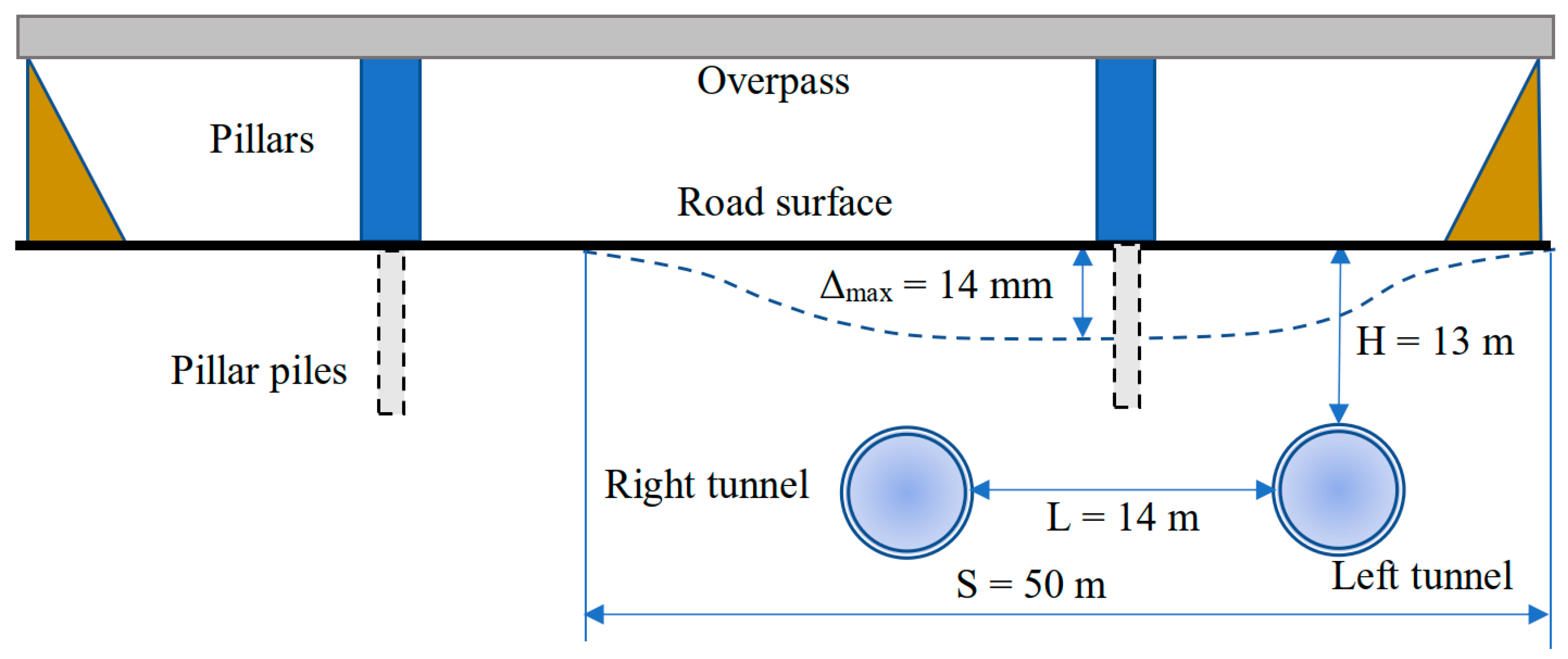
The working depth of the TBMs was 13 m from the top of the tunnel lining. The tunnels were laid out at a distance of 14 m apart in the region of the interchange, to prevent the construction works right under the pillars of the interchange overpass (Figure 2).
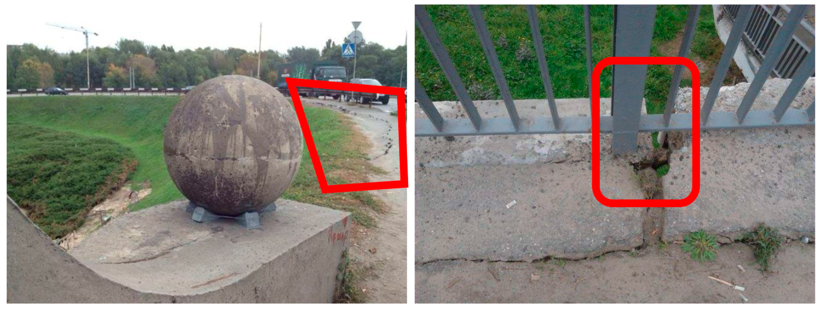
A preliminary structural and geotechnical analysis has shown that anticipated land subsidence Δmax should not have exceeded the value of 14 mm. The expected deformation zone was a circumference with a radius of 25 m and was centered under the left row of pillars. However, after the beginning of construction works in proximity to the interchange, many cracks in the overpass surface and the surrounding ground failures were observed (Figure 3). Moreover, the overpass demonstrated evidence of displacements in the horizontal plane.
The decision on the establishment of geospatial monitoring was accepted. The robotic total station was set up on the pillar, approximately 40 m from the overpass (see Figure 1). The geodetic network around the interchange was created. The observations commenced at the end of August 2012 and lasted almost three months, until both TBMs left the interchange zone, and the observable displacements tended to stabilize. For the monitoring, two observation areas (A and B) were assigned (Figure 4).
In total, fifteen deformation targets (reflectors) were set up on the pillars (Figure 5) and overpass slab (Figure 6).
This observation scheme allowed us to reliably and with necessary accuracy determine the spatial displacements of the overpass. A detailed description of this overpass’s geospatial monitoring design and accuracy analysis may be found in [16]. In an appliance from [16], the accuracy of displacement determination along the X, Y, and Z axis was equal to 1.2 mm. This value is vitally important, as it determines the errors allowable in the analysis and prediction model simulations.

3. Initial Data for Model Simulations

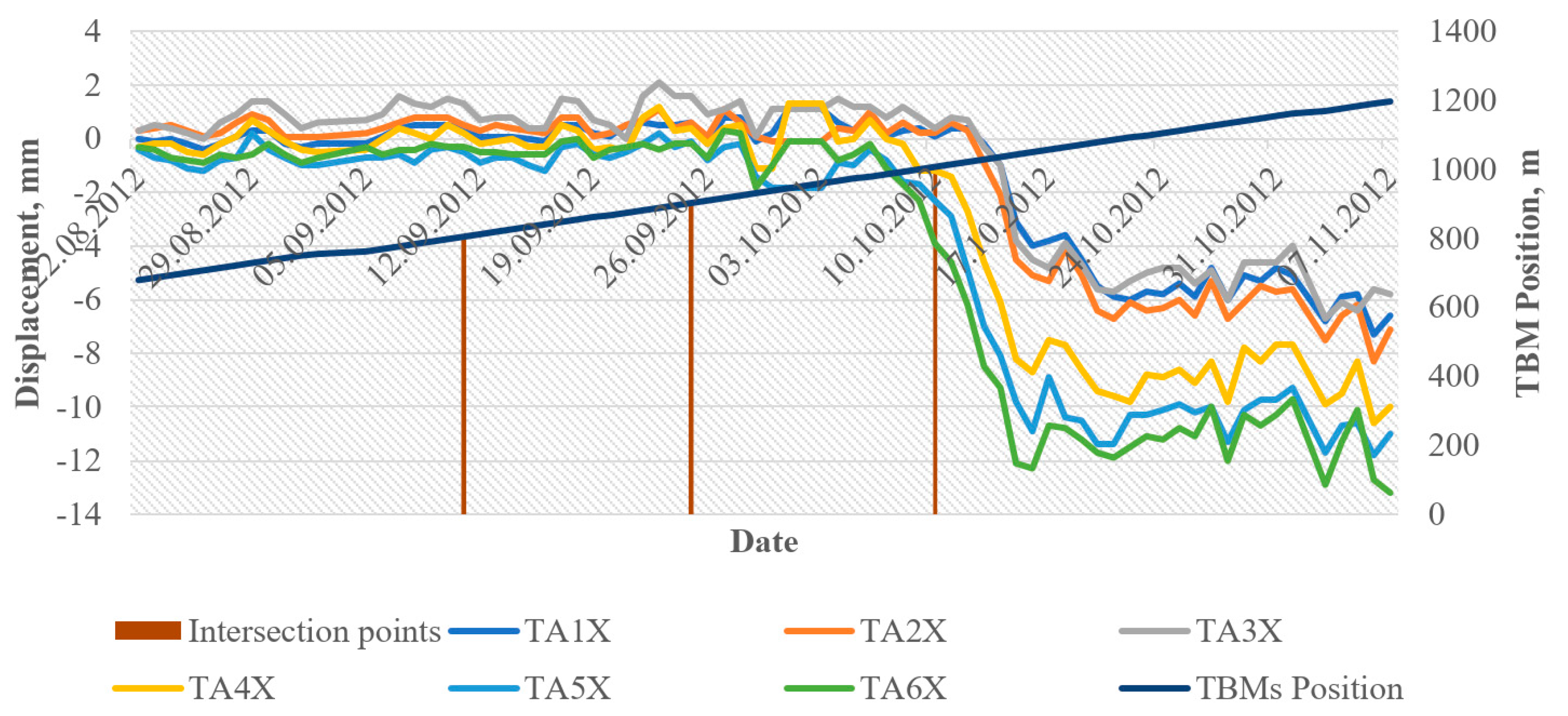
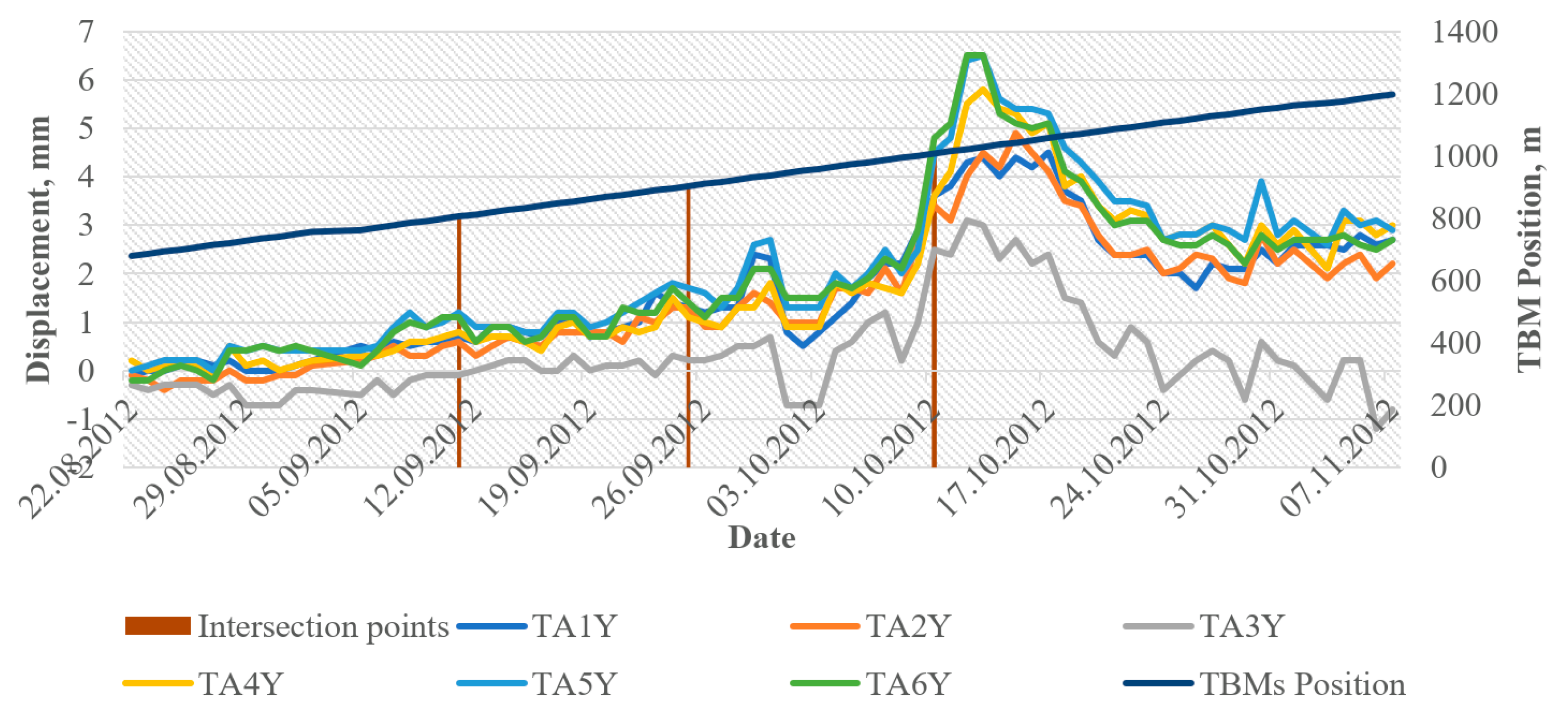
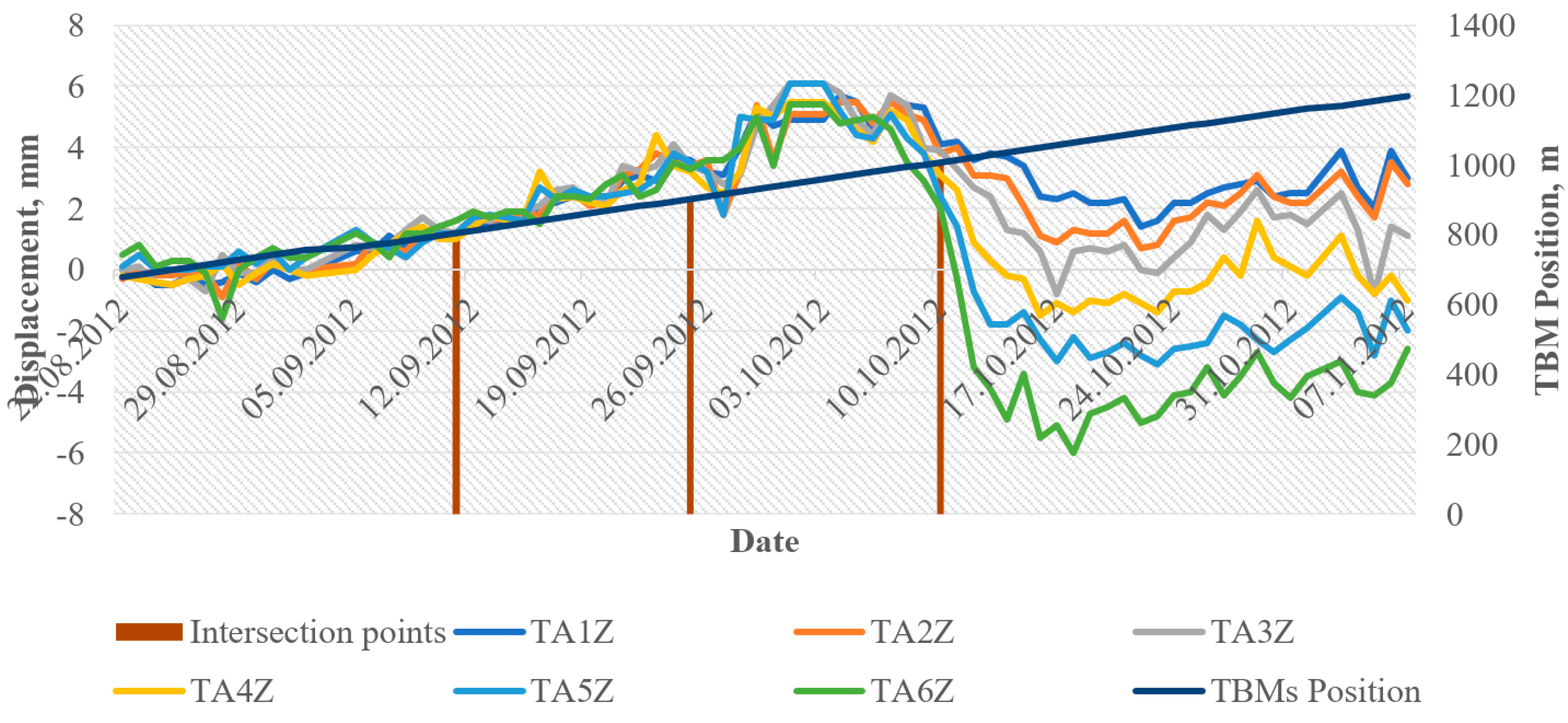
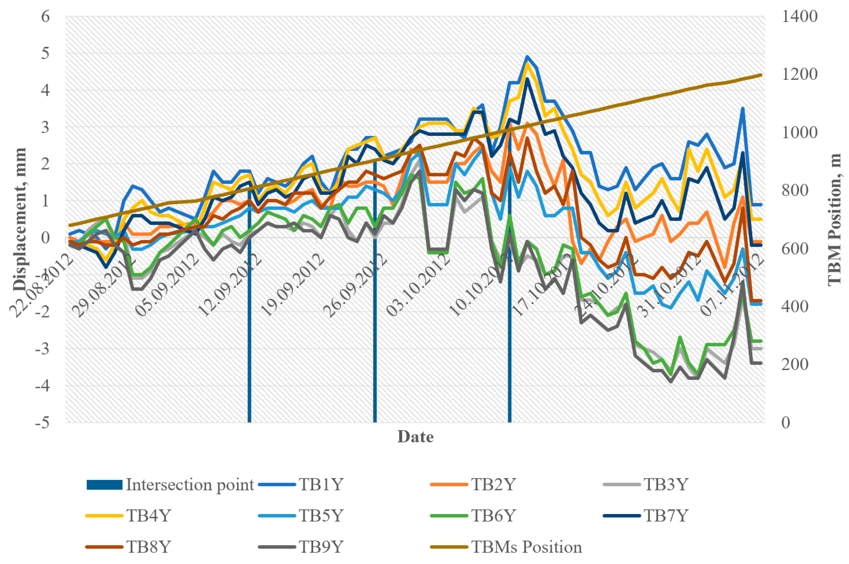
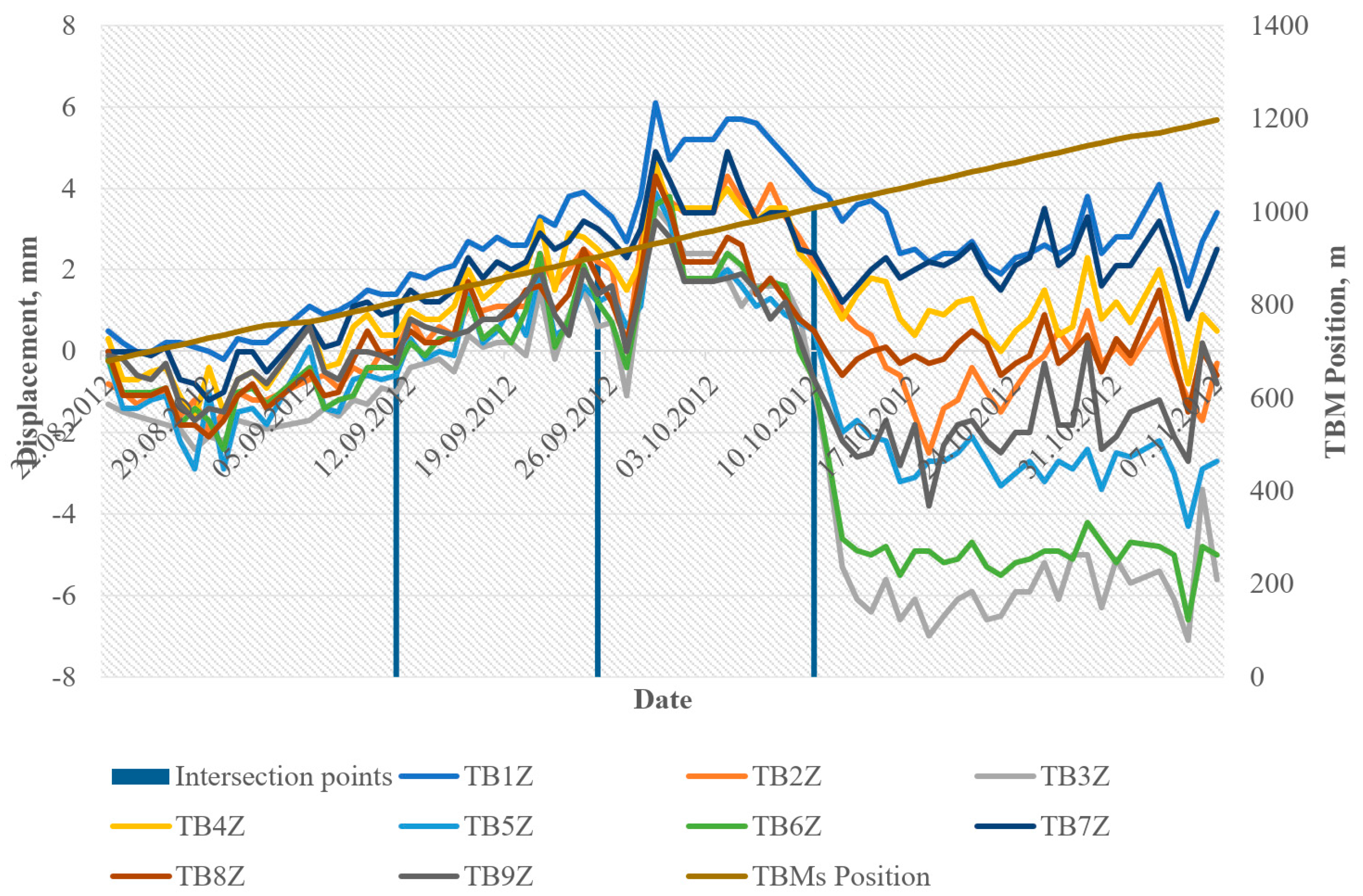
The overpass monitoring was accomplished during subway construction under the overpass. The data were collected in automatic mode by a robotic total station. As mentioned above, the data for model simulations are spatial displacements, precipitation level, temperature variation, TBM position, and subsidence coefficient (a precalculated value). Spatial displacements are by far the primary data source for simulation. Over three months, the total station determined coordinates of the deformation targets in automatic mode. The measurements were accomplished with a frequency of 30 min and then averaged daily. Those values were used for the displacement calculation along the coordinate axis. The displacements along the X, Y, and Z coordinate axes for the right tunnel (see Figure 1) are presented in Figure 7, Figure 8 and Figure 9 and in Figure 10, Figure 11 and Figure 12 for the left tunnel. The position of the TBMs is also given in Figure 7, Figure 8, Figure 9, Figure 10, Figure 11 and Figure 12. The intersection points mark the date TBM reached the middle of the interchange and the overpass, respectively. The left and right vertical lines mark the points at which TBM reached and left the interchange zone.
As shown in Figure 7, Figure 8, Figure 9, Figure 10, Figure 11 and Figure 12, for the overpass slab (area B), the deformation process commenced when construction works began near the interchange, and tended to continue when the active construction works moved further out of the interchange zone. However, the primary trend demonstrates a slight uplift and horizontal displacements, changing to tangible subsidence and horizontal movements. Meanwhile, the deformation evolved significantly for the pillars row (area A) when the active construction works moved out of the interchange zone. Again, insignificant uplifts were detected, which shifted to the subsidence.
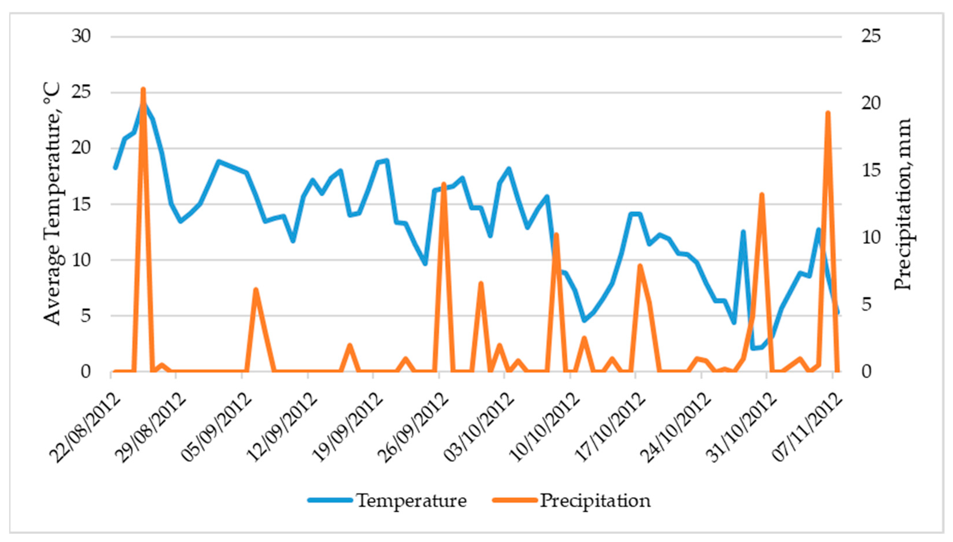
The third and fourth parameters for the simulation are temperature variation and precipitation level. For the temperature, the daily average value was used. For the precipitation level, the daily cumulative value was used. Both parameters were tabulated, and their charts are given in Figure 13.
One more additional parameter was derived empirically. The subsidence coefficient relates to the TBM’s position and the precalculated land subsidence value due to excavation works (see Section 2, Figure 1 and Figure 2).
S C T B M = Δ i T B M Δ m a x ,
where Δ i is a current precalculated value of land subsidence.
The suggested subsidence coefficient is equal to zero until the TBM reaches the interchange, then starts to increase linearly when land subsidence grows; it becomes one when the TBM reaches the interchange middle point (Figure 14).
The data presented above have been used to simulate different prediction models using regression analysis and neural network regression using machine learning methods. The following section outlines the simulation results in detail.

4. Results and Discussions

4.1. Regression Analysis Results

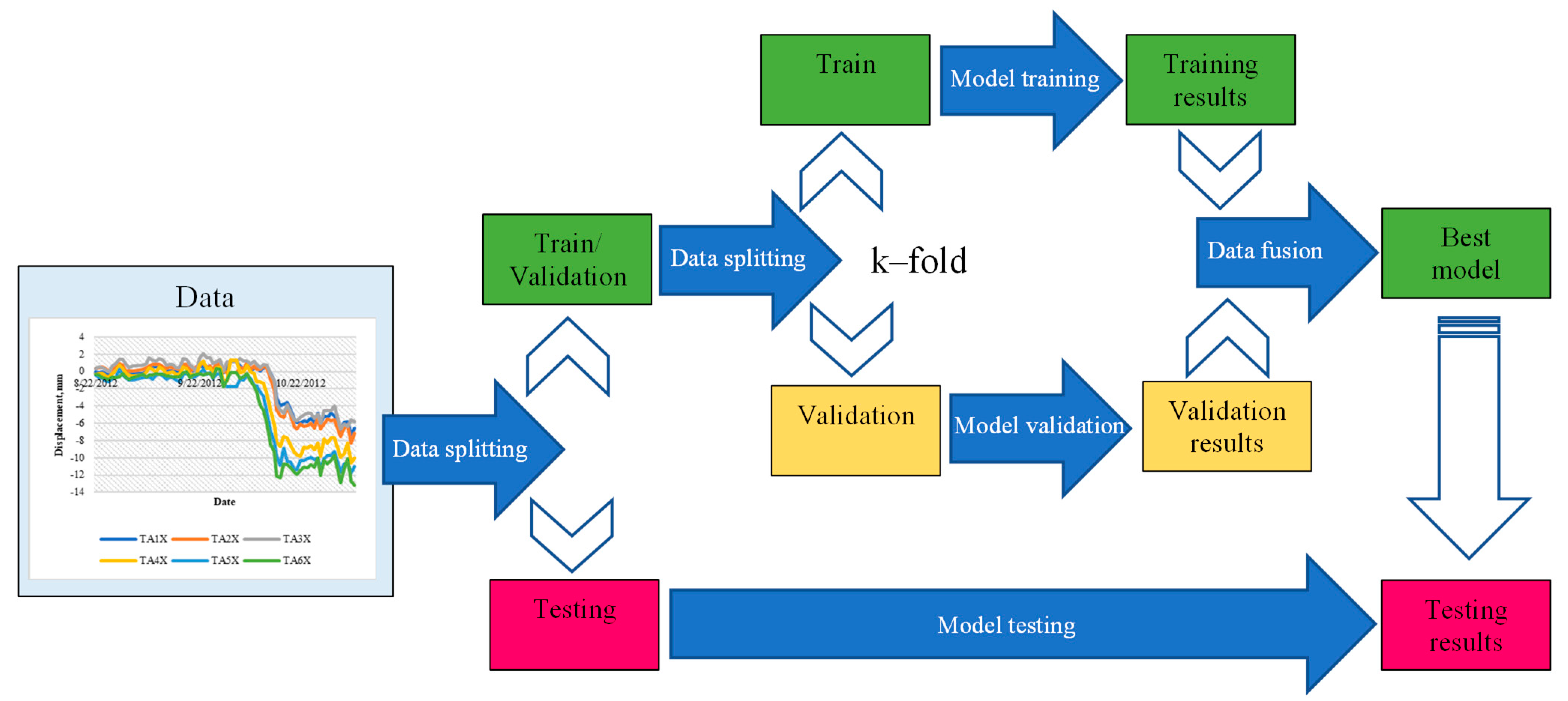
The first method considered for the simulation of prediction models is regression analysis with machine learning. Insofar as the primary goal of the analysis is the prediction of spatial displacements using geospatial monitoring data, the displacements are treated as responses, while other parameters are predictors or features. The critical question is the choice of the learning algorithm. As long as the data volume is not significant (75 observations), we decided to apply a k-fold validation procedure for learning. The number of folds was accepted to be eight. Another challenge is splitting the data into training, validating, and testing data subsets. Again, considering the data size, the following percentages for the subsets were suggested: a training/validation ratio of 80/20, and testing subsets of 15%. The machine learning flowchart suggested in this study is given in Figure 15.
Multiple linear regression models have been chosen from the diversity of regression models. A visual analysis of the data presented in Section 2 showed that the displacements have mostly linear or squared trends. This is why two multiple linear regression models were considered.
f x , β = β 0 + β 1 T + β 2 P + β 3 S + β a T B M ,
f x , β = β 0 + β 1 T 2 + β 2 P 2 + β 3 S 2 + β a T B M 2 ,
where T ,   P ,   S ,   T B M are the temperature, precipitation, subsidence coefficient, and TBM position, respectively.
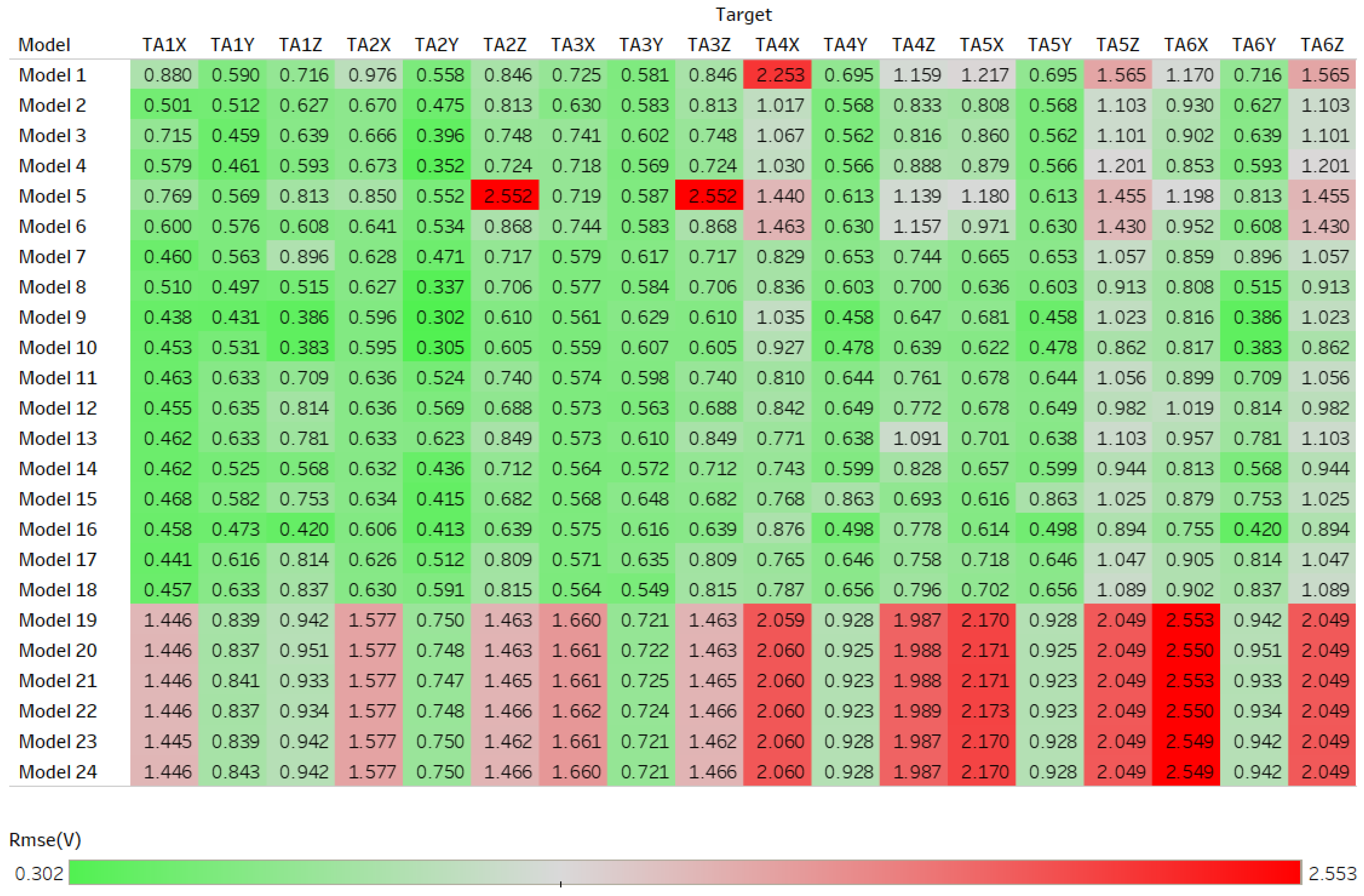
The simulation has been accomplished separately for all deformation targets. The regression learning was carried out for different calculation approaches. The following approaches for the simulation were considered: simple multiple linear regression, robust multiple linear regression, multiple linear regression with interactions, stepwise multiple linear regression, and quadratic regression. The simulation results have been tabulated. The estimations are given for validation and testing data subsets for each model. Three statistical metrics were calculated to estimate the validation results: mean absolute error, root mean square error, and coefficient of determination. The root mean square error and coefficient of determination were used for model evaluation. The mean absolute error was considered when two or more models delivered similar statistical metrics. Let us present the root mean square error metrics for learning validation cases. Figure 16 and Figure 17 demonstrate colorized tables, wherein colors are assigned according to the threshold values. For the root mean square error, the threshold value is 1.2 mm. Regarding the comments in Section 2, this value corresponds to the measurement accuracy. Therefore, any root mean square error that exceeds the threshold is considered unallowable. Consequently, the green cells correspond to allowable values, and the red cells do not. For the coefficient of determination, the threshold value is 0.7. Below this threshold, the values are not acceptable. Those models for which one or both values do not satisfy the given criteria are considered failed. Following the link https://public.tableau.com/views/RegressionValidationA/RegValidationDA?:language=en-US&publish=yes&:display_count=n&:origin=viz_share_link (accessed on 20 September 2023), one may study the mean absolute error and coefficient of determination metrics for area A. The mean absolute error and coefficient of determination metrics for area B are available through https://public.tableau.com/views/RegressionValidationB/RegressionValidationDB?:language=en-US&publish=yes&:display_count=n&:origin=viz_share_link (accessed on 20 September 2023).
The following designators are used in Figures and links: Rmse—root mean square error, Rsq—coefficient of determination, (V)—estimation for the validation data subset.
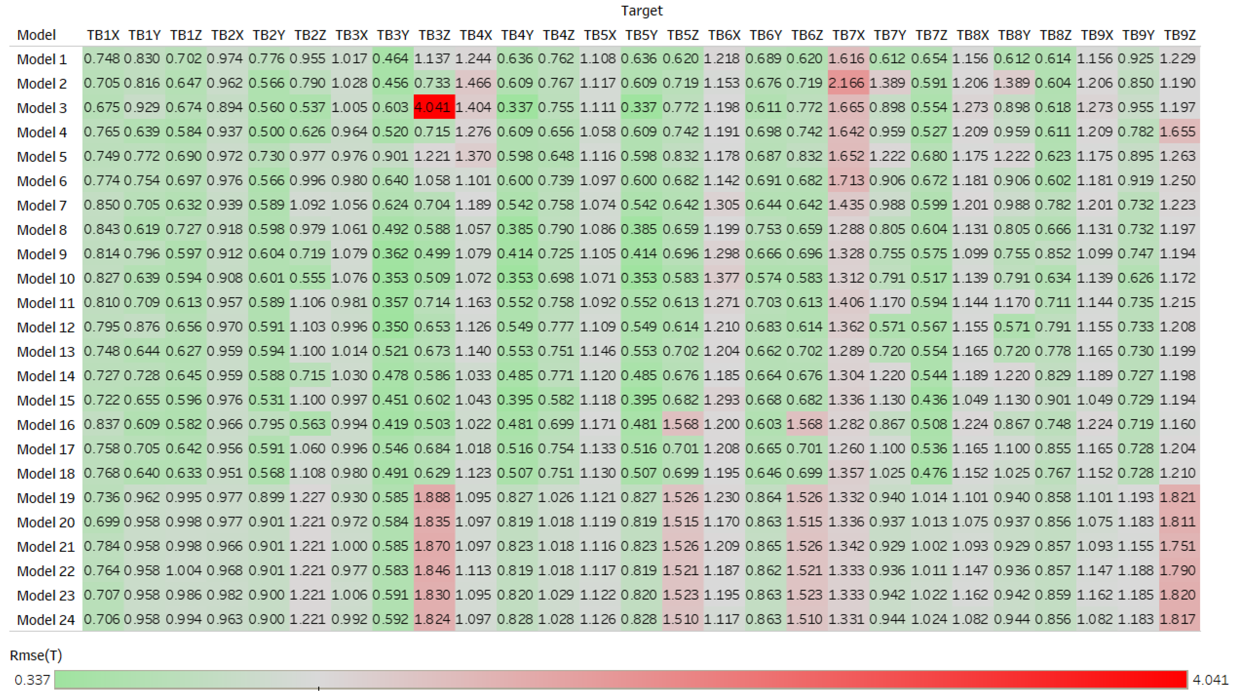
Figure 18 and Figure 19 demonstrate the root mean square errors for the testing data subset (T). The tabulated and colorized information about evaluation metrics for testing is available through the link https://public.tableau.com/views/RegressionTrainingA/RegressionTrainingDA?:language=en-US&publish=yes&:display_count=n&:origin=viz_share_link (accessed on 20 September 2023), for area A, and through the link https://public.tableau.com/views/RegressionTrainingB/RegR2TrainingDB?:language=en-US&publish=yes&:display_count=n&:origin=viz_share_link (accessed on 20 September 2023), for area B. For the testing data, the same threshold values were assigned.
The preliminary analysis shows the low efficiency of the regression models. No model provides acceptable values for all deformation targets. Moreover, there are many cases in which no regression model ensures the assigned criteria at all. An in-depth discussion of the presented results is given in Section 4.3.

4.2. Neural Network Regression Results

Neural network regression provides more flexible tools for simulation tuning. Thanks to the wide set of hyperparameters, neural network regression allows the simulation of more complex data. For our case study, the following hyperparameters were examined: activation function, number of layers, and number of outputs in each layer. The network type is a feedforward, fully connected neural network. Four activation functions were considered:
  • rectified linear unit function f x = x ,   x 0 0 ,   x < 0 ;
  • hyperbolic tangent function f x = e x e x e x + e x ;
  • the sigmoid function f x = 1 1 + e x ;
  • identity function f x = x .
Apart from the given activation functions, different numbers of layers and outputs were studied. These hyperparameters create sets of various combinations. These combinations are numbered as models and are listed in Table 1.
For all of the models from Table 1, the neural network regressions have been trained according to the flowchart in Figure 15. The threshold criteria were accepted the same as for the regression analysis. Figure 20 presents the root mean square errors for the data validation subset of area A. Figure 21 gives the same metrics for area B. One may find the complete set of simulation metrics (mean absolute error, root mean square error, and coefficient of determination) via the links https://public.tableau.com/views/NeuNetValidationA/NeuNetValidationDA?:language=en-US&publish=yes&:display_count=n&:origin=viz_share_link (accessed on 20 September 2023), for area A, and https://public.tableau.com/views/NeuNetValidationB/NeuNetValidationDB?:language=en-US&publish=yes&:display_count=n&:origin=viz_share_link (accessed on 20 September 2023) for area B.
If we compare the neural network regression with the regression analysis, we may notice that the neural network regression demonstrates much better performance than a simple regression. However, these results correspond to the validation data subset. Let us look at the output of the neural network regression for the testing data subsets. The model testing results for areas A and B are presented in Figure 22 and Figure 23. One may find the complete set of simulation metrics (mean absolute error, root mean square error, and coefficient of determination) via the links https://public.tableau.com/views/NeuNetTestingA/NeuNetTestingDA?:language=en-US&publish=yes&:display_count=n&:origin=viz_share_link (accessed on 20 September 2023), for area A, and https://public.tableau.com/views/NeuNetTestingB/NeuNetTestingDB?:language=en-US&publish=yes&:display_count=n&:origin=viz_share_link (accessed on 20 September 2023), for area B.
Even though the model testing results are not as optimistic as for the validation data subset, the neural network regression has considerably better accuracy than a simple regression model. A discussion of the results presented above is given in the following subsection.

4.3. Best Model Performance Analysis and Discussions

Using the obtained results, an in-depth analysis is possible. The main goals of the analysis and discussion are two: the first is to determine the approach that ensures better results, and the second is to suggest the best set of parameters and hyperparameters. A visual analysis of the results in Section 4.1 and Section 4.2 has shown that linear regression analysis models generally ensure inappropriate results. To comprehend the efficiency of the linear regression analysis and to prove it qualitatively, the best regression model has been chosen for each deformation target. When no one regression model satisfies the assigned threshold values for the specified deformation target, the simulation for this target fails. Thus, there are no linear regression models that may describe the deformation process, respectively. The results of such a survey are outlined in Table 2 for area A and Table 3 for area B. The failed simulations are designated (F).
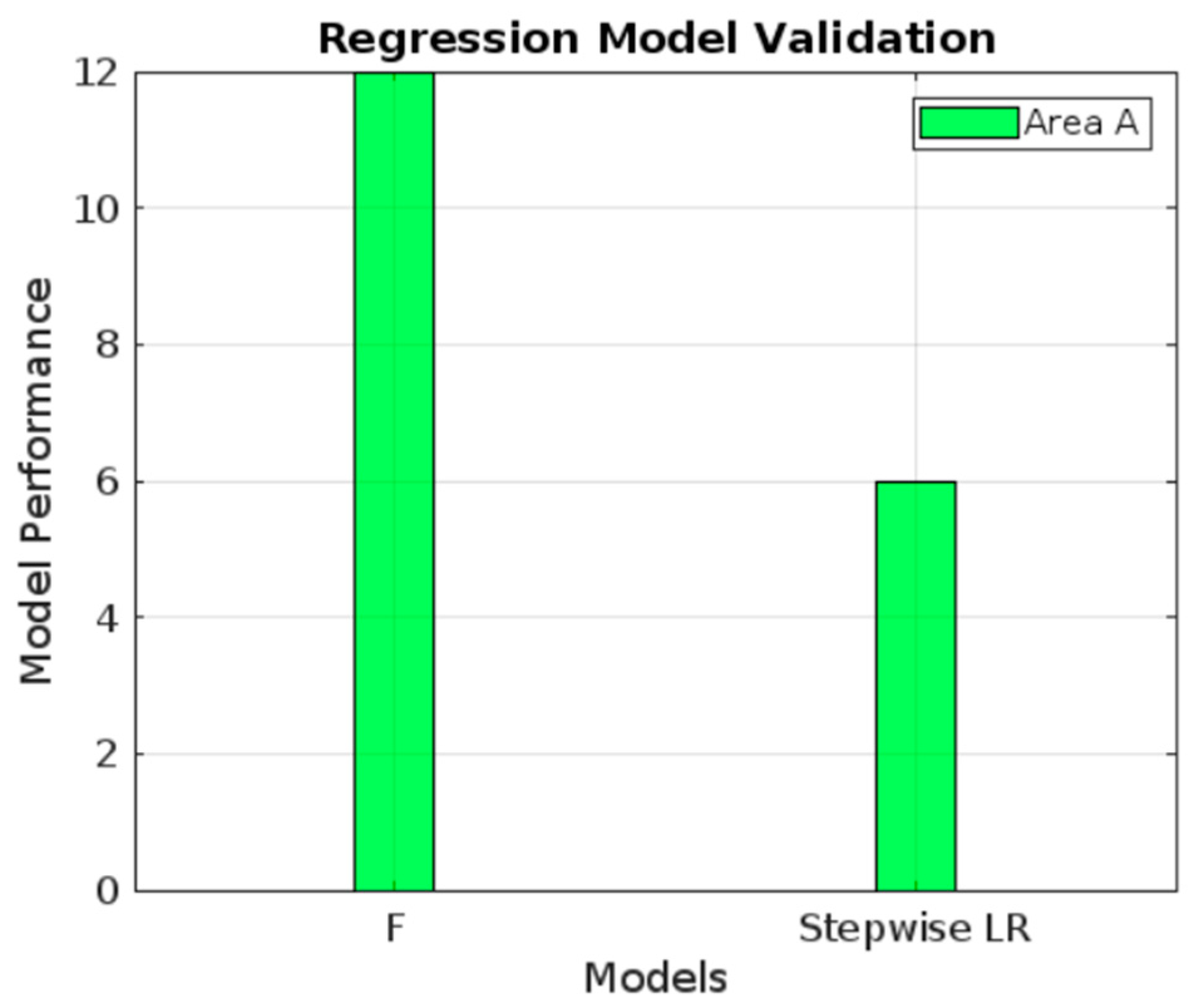
The data in the tables above are presented in histogram view. The histograms have been built for the validation and testing data of areas A (Figure 24 and Figure 25) and B (Figure 26 and Figure 27). These Figures provide a presentable overview of the different model performances.
The regression models’ performance for area A is mostly poor. No one model is able to ensure reliable results.
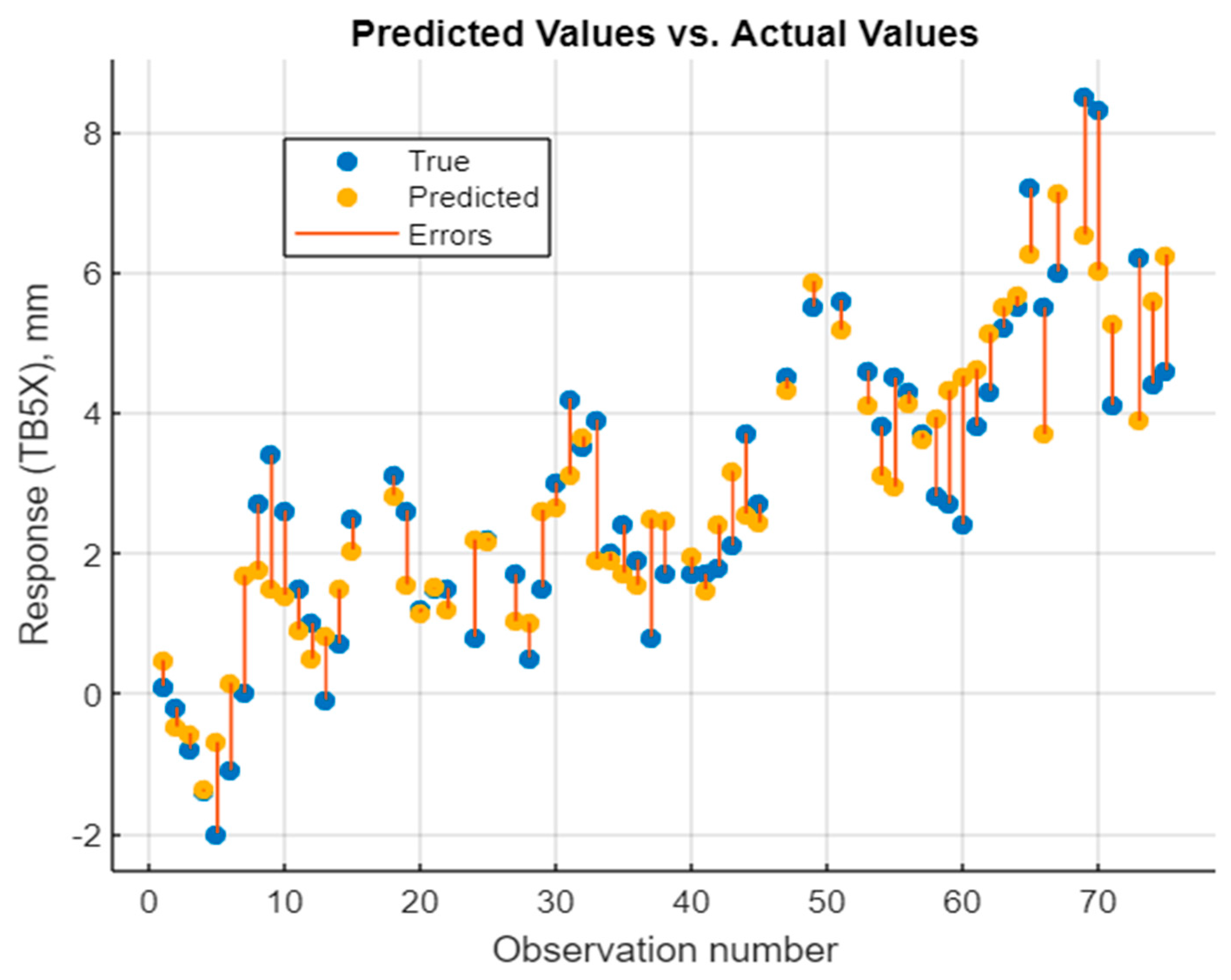
There is no doubt that regardless of the monitoring area, the linear regression analysis mostly fails to describe and predict the overpass displacements due to land subsidence. In monitoring area A, more than half of the simulations failed (see Figure 24 and Figure 25). There is no relationship between the coordinate axis or displacement direction and model performance (see Table 2). Stepwise linear regression provides the most stable solution for the validation data subset among the different linear regression models. In contrast, quadratic linear regression is more suitable for the testing data subset. However, in both cases, the percentage of successful models is just 30%. The results of area B show a slightly different trend. Stepwise linear regression is successful for more than 50% of cases for the validation data subset (Figure 26), but the percentage of failed simulations is still inadmissibly high (more than 40%). The percentage of the failed simulations for the testing data subset is almost 50% (Figure 27). Critical remarks should be made regarding the simulations along different coordinate axes. It was found that stepwise linear regression works pretty well for the displacement simulation along the X-axis. Let us see the simulation output for the stepwise linear regression for the deformation target TB5 along the X-axis. Figure 28 portrays the determined displacements and predicted displacements compiled using stepwise linear regression.
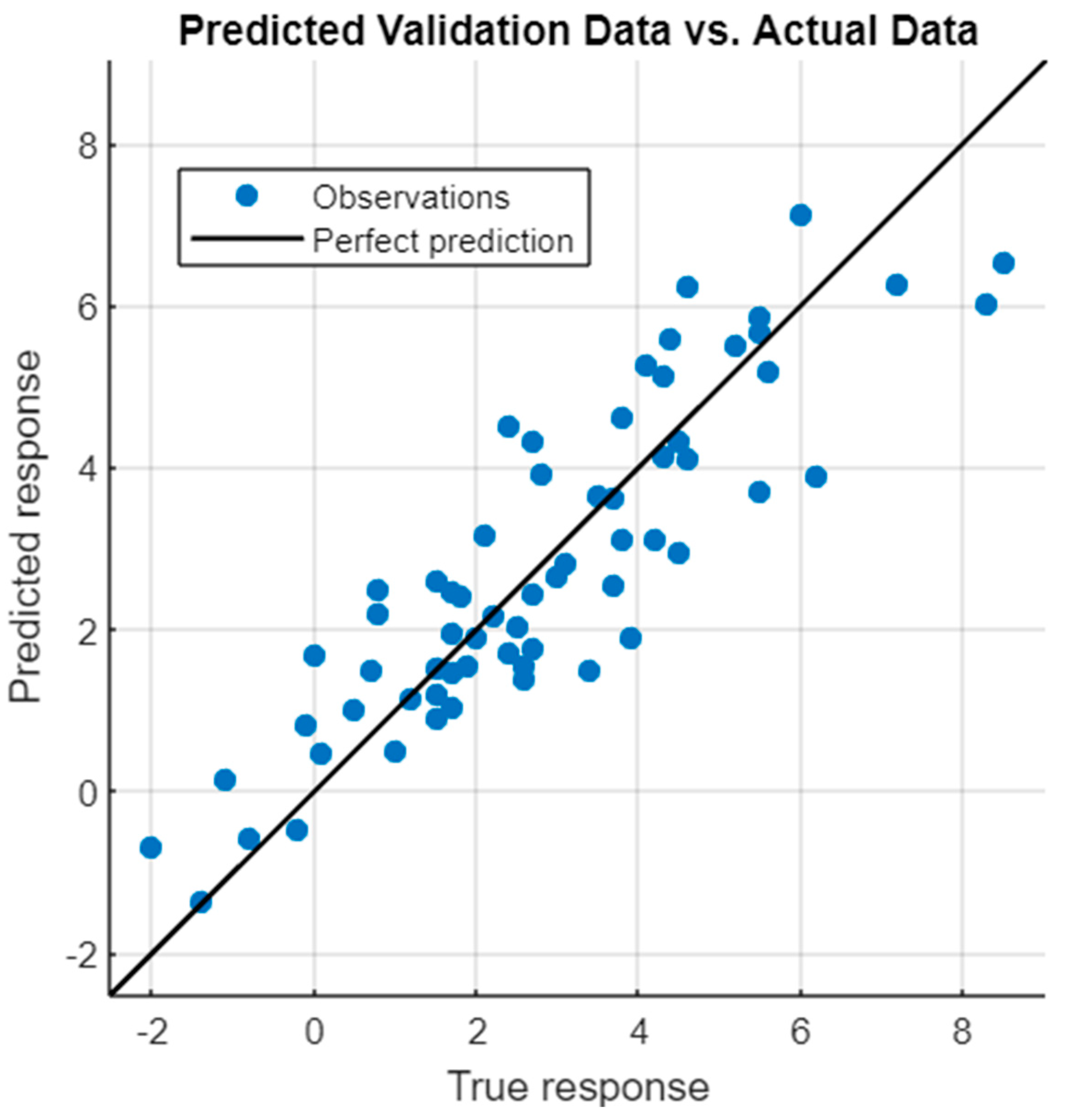
The relationships between the actual and predicted responses are given in Figure 29 and Figure 30.
The responses for the validation and testing data subsets are grouped along straight lines. If we assume that our regression model is correct, then most of the data (displacements) variability is explained by this model. Consequently, the choice of parameters and their relationships was correct.
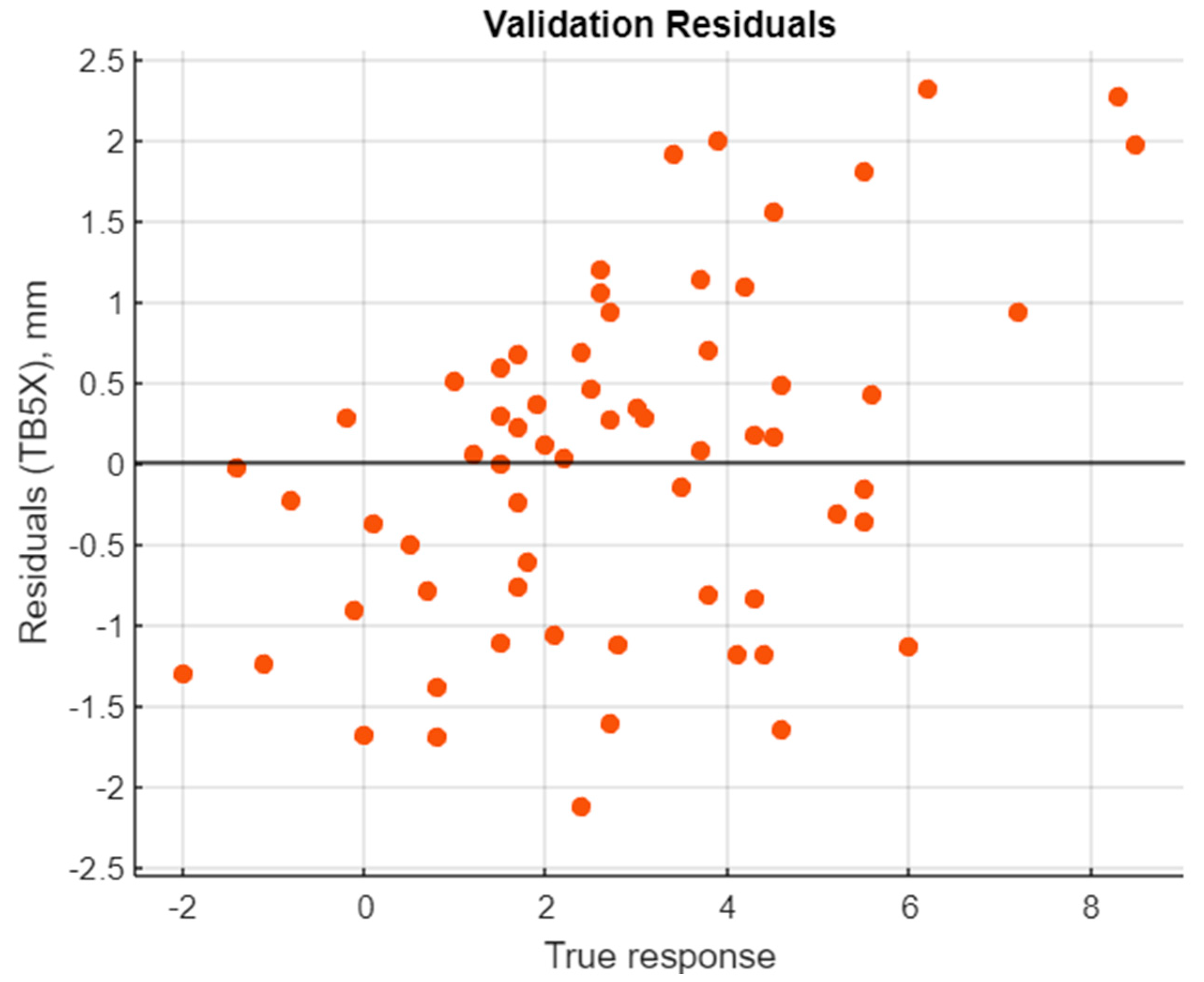
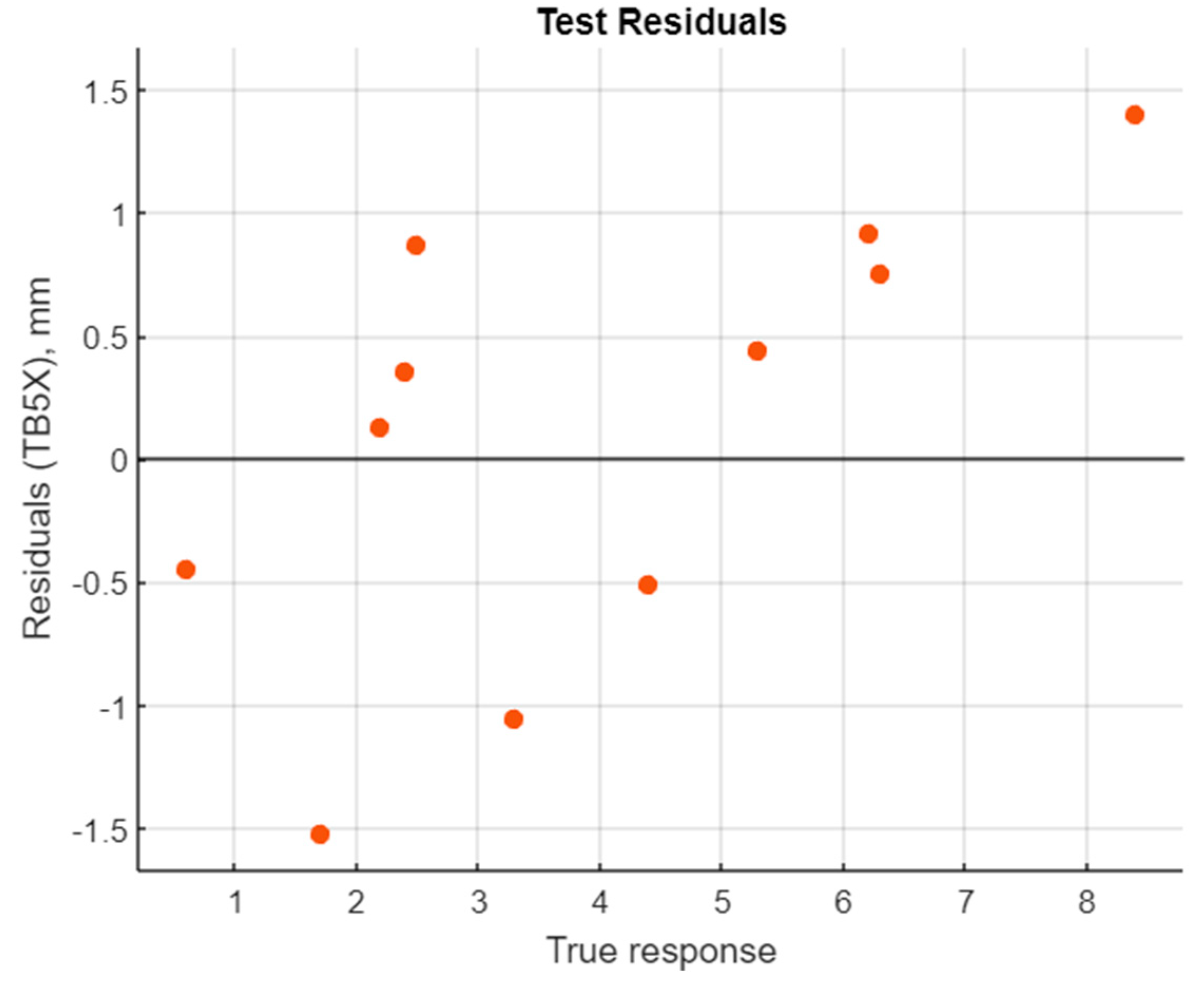
The residuals between actual and predicted values give a nice view of the model’s efficiency. The residuals for the validation and testing data subsets are given in Figure 31 and Figure 32.
The residuals for the validation data subset do not exceed the doubled accuracy of the displacements. The distribution of the residuals shows no systematic trends or blunders. In general, we may infer that the stepwise linear regression appropriately describes the displacements of this particular deformation target. Therefore, if a model obeys the assigned thresholds, the simulation results are adequate for the deformation process. The prediction model is not underfitted nor overfitted. This means that linear regression is capable of grasping the main trends of the deformation process. The same conclusions are valid for the testing data subset. The parameters’ importance scores were estimated using F-test (Figure 33).
For this particular case, precipitation is the only parameter we must neglect. This is evident because during monitoring, the precipitation level was not significant, and consequently should not affect the observable displacements. All the rest of the parameters have high importance scores. Despite the presented results, the studied linear regression models generally do not provide suitable outputs. One of the reasons for this is the insufficient number of regression parameters. Consequently, we must admit that the suggested regression models are underfitted in general. Thus, additional regression parameters, e.g., transport loads, soil parameters, etc., must be included to grasp hidden trends in monitoring data. Another probable solution is the use of nonlinear regression models.
Let us embark on an analysis of the neural network regression results. As in the case of simple regression, all simulation results have been checked, and the best model for each deformation target has been chosen. The results of this selection are shown in Table 4 and Table 5.
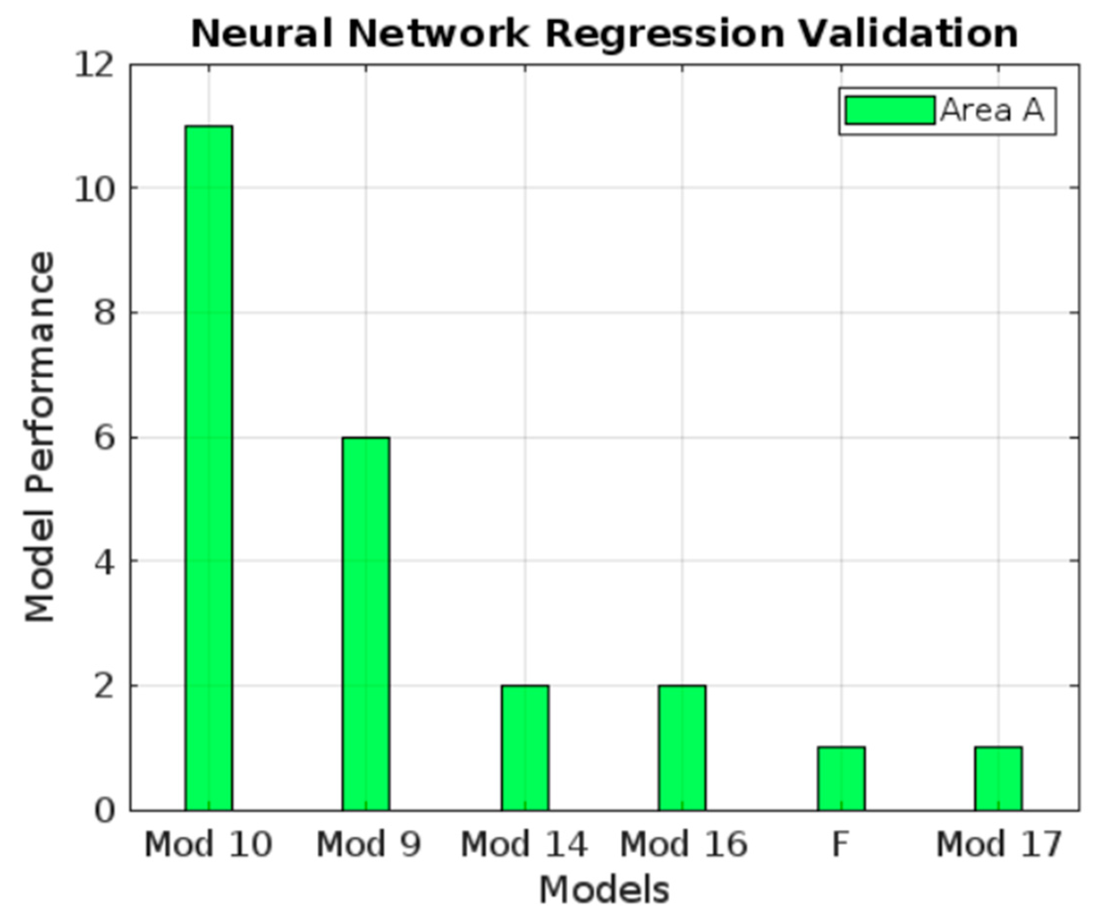
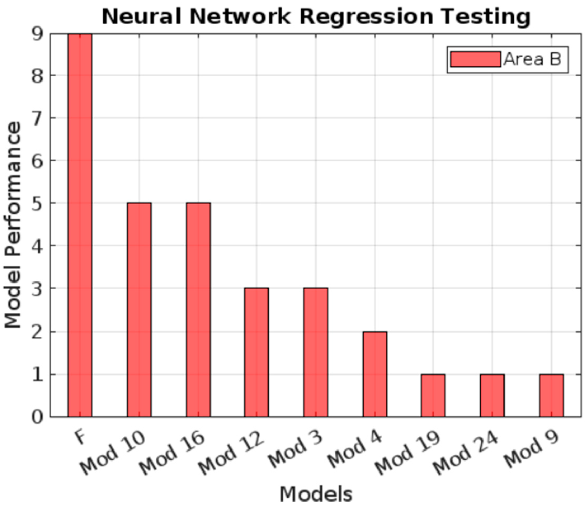
The data in the tables above are presented in a histogram view. The histograms have been built for validation and testing data for areas A (Figure 34 and Figure 35) and B (Figure 36 and Figure 37).
For areas A and B, we have totally different pictures. Area A has only one failed simulation for the validation and testing data subsets. The highest performance for the validation data ensures Model 10 (a one-layer network with twenty outputs and hyperbolic tangent activation function) and Model 9 (a three-layer network with ten outputs in each layer and hyperbolic tangent activation function). The success of these models is almost 75%. If we look at the testing data, there is no apparent domination of one model in favor of another. However, 50% of successful simulations correspond to models with hyperbolic tangent activation function, and 30% correspond to those with sigmoid activation function. For deformation processes similar to those in area A, it is advisable to use neural network regression with hyperbolic tangent or sigmoid activation functions. The number of layers and outputs is not so critical. It is recommended to apply networks with one or two layers. The output number must be between ten and thirty. It is undesirable to apply a rectified linear unit function and identity function. The latter failed almost all simulations for the studied data sets.
As a case study of the neural network regression performance, let us consider the simulation results for the deformation target TA6 along the X-axis. Figure 38 demonstrates the determined and predicted displacements compiled using neural network regression for Model 16 (sigmoid activation function, three layers, and thirty, twenty, and ten outputs, respectively).
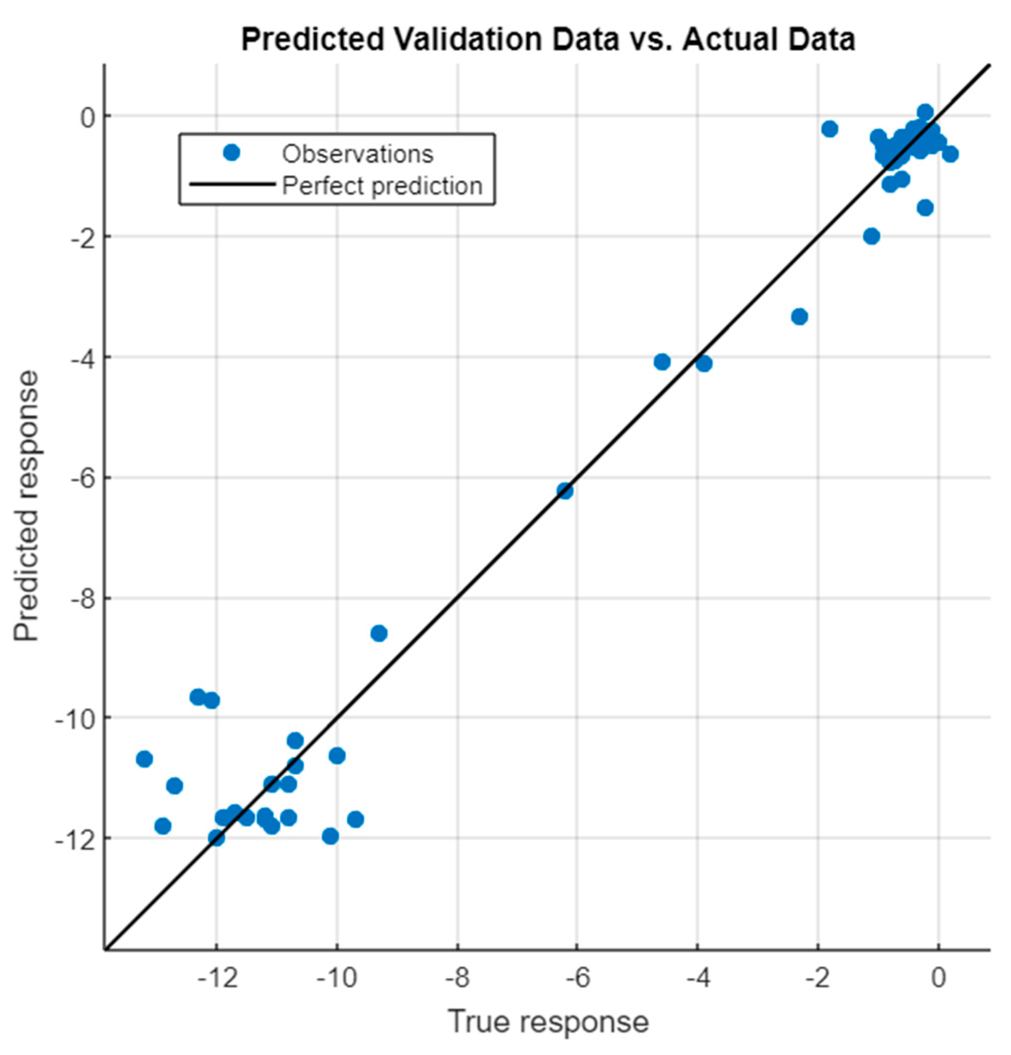
The relationships between the actual and predicted responses are given in Figure 39 and Figure 40.
The responses for the validation and testing data subsets are grouped along straight lines. The residuals between actual and predicted values give a nice view of the model’s efficiency. The residuals for the validation and testing data subsets are given in Figure 41 and Figure 42.
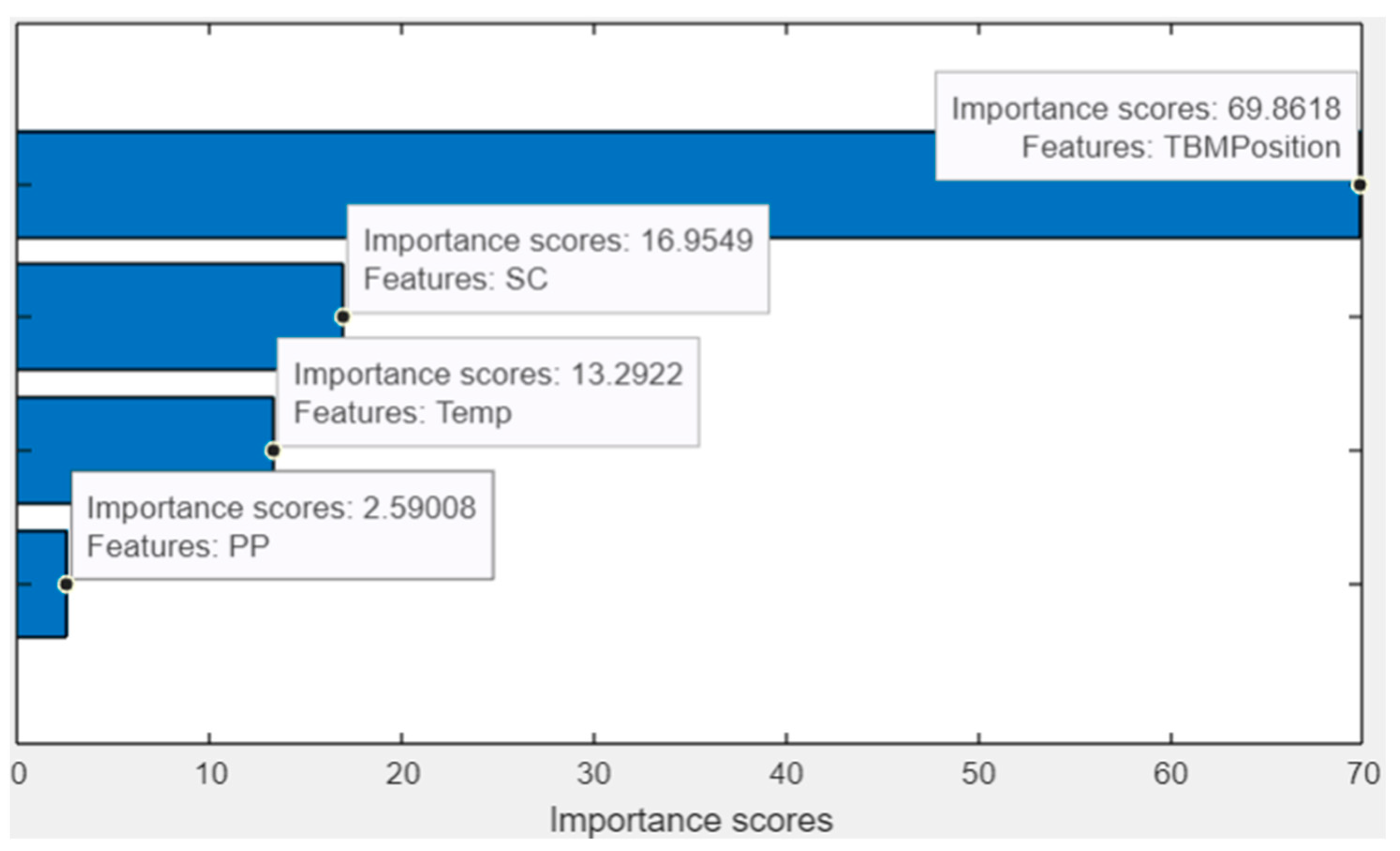
The residuals for the validation data subset almost fit into the region of the doubled accuracy of the displacements (±2.4 mm), while the residuals for the testing data subset are in the range of ±1 mm. The distribution of the residuals has no systematic trends or blunders. The prediction model is not underfitted or overfitted. The parameters’ importance scores were estimated using an F-test (Figure 43).
For this case, precipitation again has the lowest score, and should be neglected. All the rest of the parameters have high importance scores. Neural network regression mainly provides acceptable results. However, the inclusion of additional parameters is also advisable.
For area B, we may observe a significant percentage of failed simulations. This percentage equals 17% for the validation data subset and 33% for the testing data subset. The most successful models are with sigmoid activation function: 37% for the validation data subset, and 20% for the testing data subset; and with hyperbolic tangent activation function: 28% for validation, and 20% for testing. Again, the number of layers and outputs is not so critical. Conclusions regarding the number of parameters drawn from the linear regression analysis are also valid for the neural network regression. Through the inclusion of new parameters, we may improve the simulation quality.
For the case of neural network regression, we have an additional option for tuning the hyperparameters. Thus, we may reach the necessary threshold criteria by varying the number of layers and outputs. In this case, we deal with optimizable neural network regression. We took the deformation target TB8 and its displacements along the Z-axis to prove this statement. Both validation and testing procedures for the standard neural network regression failed to reach this target. Let us run the optimization process and search the optimal number of layers and outputs for hyperbolic tangent and sigmoid activation functions. Additionally, we have increased the number of cross-validation folds to ten. The optimization of the number of outputs shows acceptable results. The simulation results indicate that the optimizable neural network regression can adjust the hyperparameter values to satisfy the threshold values. Figure 44 shows charts of the mean square errors (MSEs)’ optimization for successful hyperparameters.
The obtained values for the hyperparameters that satisfy the assigned criteria are outlined in Table 6.
Figure 45 demonstrates the determined and predicted displacements compiled with the optimizable neural network regression.
There is no significant difference between networks with various hyperparameters. This means that any of the neural network models in Table 6 may be used for the prediction model. The earlier discussion implies that the optimizable neural network regression is considerably flexible, and additionally provides lower values for root mean square errors and mean absolute errors (see Section 4.1). The obtained evidence seems to recommend that the optimizable neural network regression simulation must include the following steps:
(1)
Assigning the validation procedure. For small datasets (up to 300 responses), this is a k-fold validation with at least ten folds, and for large datasets (more than 1000 responses), a hold-out validation procedure.
(2)
Assigning the testing data subset, which is 15–20%, depending on the dataset size.
(3)
Choosing the set of parameters (predictors).
(4)
Choosing the optimizable hyperparameters (activation function, number of layers, and outputs).
(5)
Assigning the activation function (hyperbolic tangent or sigmoid).
(6)
Optimizing the number of layers and the number of outputs.
(7)
Comparing the estimation metrics.
Generally speaking, optimizable neural network regression is the best solution for creating prediction models compared to ordinary regression.
The urban environment is prone to continuous changes. The construction processes affect the surrounding structures and lead to ground displacements. On the other hand, adverse geological and meteorological conditions may overplay the construction process and make city management a complex issue. These conditions dictate the usage of the models that allow the parameters to be tweaked and the algorithms to be adjusted depending on the changes. Optimizable neural network regression models are applicable for simulating various deformation processes. In an urban environment, these models may successfully describe not only land subsidence but also bridge deformations subject to static and dynamic loads, high-rise building deformations that may undergo extreme environmental loads (temperature, wind gusts, etc.), and underground structure displacements.
The studied models and the suggested optimizable neural network regression are recommended as an indispensable part of geotechnical monitoring. Practically, after each new observation epoch, these models allow for on-the-fly estimation of the structure deformation process or land subsidence. Therefore, it is highly recommended to embed these models into software for the analysis of monitoring results.

5. Conclusions

Land subsidence in cities may lead to significant damage to and collapsing of engineering structures. The simulation and prediction of these structures’ deformations due to land subsidence is a great challenge. The present paper addresses the problem of applying machine learning methods for analyzing spatial displacements of engineering structures. The results of geospatial monitoring of a road overpass affected by external loads invoked by the construction of a new subway line were used as a case study. The primary stress has been placed on applying machine learning methods for the development of a prediction model. Two methods have been examined: regression analysis and neural network regression with machine learning. Regression analysis was accomplished using a k-fold cross-validation scheme with the testing data subset. The overall analysis has shown that the regression analysis does not provide the necessary accuracy and reliability of prediction models. The regression analysis learning failed for almost 50% of simulations. The main drawback is the model underfitting. One of the recommendations is increasing the number of regression parameters. Notably, the level of traffic loads, underground soil structure, subsidence parameters due to underground excavation works, etc. should be considered. Unlike the regression analysis, the neural network regression ensured essentially better results. In general, only nearly 25% of the neural network regression simulations failed. Neural network regression is able to grasp the local deviations of the displacements and convey the pattern of the deformation process. Finally, optimizable neural network regression has been considered. The study found optimizable neural network regression to be highly reliable. Thanks to the optimization procedure, it is almost possible to adjust the hyperparameters of the neural network in such a way that its output will satisfy the preliminary assigned criteria. As a general conclusion, we recommend using optimizable neural network regression methods to construct prediction models. In future, research will have to address machine learning methods for analyzing spatial displacements in more detail. Perspective studies will have to explore deep learning methods for the development of prediction models. Of course, future studies will have to concentrate on the issue of parameter choice for correct data simulation and to prevent models’ underfitting.

Author Contributions

Conceptualization, R.S.; methodology, R.S., M.B. and A.A.; software, A.O., A.K. and R.A.; validation, A.O., A.K., T.N. and R.A.; formal analysis, R.S. and A.A.; investigation, M.B., A.O., A.K. and A.A.; resources, M.B.; data curation, M.B.; writing—original draft preparation, A.O., A.K., A.A. and R.A.; writing—review and editing, R.S. and T.N.; visualization, R.S., T.N. and R.A.; supervision, R.S.; project administration, R.S. and M.B.; funding acquisition, M.B. All authors have read and agreed to the published version of the manuscript.

Funding

This research received no external funding.

Data Availability Statement

The data for analysis were uploaded to Tableau Public and are available via the following links: https://public.tableau.com/views/RegressionValidationA/RegValidationDA?:language=en-US&publish=yes&:display_count=n&:origin=viz_share_link (regression validation area A, accessed on 20 September 2023); https://public.tableau.com/views/RegressionValidationB/RegressionValidationDB?:language=en-US&publish=yes&:display_count=n&:origin=viz_share_link (regression validation area B, accessed on 20 September 2023); https://public.tableau.com/views/RegressionTrainingA/RegressionTrainingDA?:language=en-US&publish=yes&:display_count=n&:origin=viz_share_link (regression testing area A, accessed on 20 September 2023); https://public.tableau.com/views/RegressionTrainingB/RegR2TrainingDB?:language=en-US&publish=yes&:display_count=n&:origin=viz_share_link (regression testing area B, accessed on 20 September 2023); https://public.tableau.com/views/NeuNetValidationA/NeuNetValidationDA?:language=en-US&publish=yes&:display_count=n&:origin=viz_share_link (neural network regression validation area A, accessed on 20 September 2023); https://public.tableau.com/views/NeuNetValidationB/NeuNetValidationDB?:language=en-US&publish=yes&:display_count=n&:origin=viz_share_link (neural network regression validation area B, accessed on 20 September 2023); https://public.tableau.com/views/NeuNetTestingA/NeuNetTestingDA?:language=en-US&publish=yes&:display_count=n&:origin=viz_share_link (neural network regression testing area A, accessed on 20 September 2023); https://public.tableau.com/views/NeuNetTestingB/NeuNetTestingDB?:language=en-US&publish=yes&:display_count=n&:origin=viz_share_link (neural network regression testing area B, accessed on 20 September 2023).

Conflicts of Interest

The authors declare no conflict of interest.

References

  1. Lepadatu, A.; Tiberius, C. GPS for structural health monitoring—Case study on the Basarab overpass cable-stayed bridge. J. Appl. Geod. 2013, 8, 65–86. [Google Scholar] [CrossRef]
  2. Ono, M.N.; Agbo, J.A.; Ijioma, D.I.; Chubado, M. Establishment of Baseline Data for Monitoring of Deformation of Murtala Mohammed Bridge (MMB) Lokoja Kogi State, using GPS. Int. J. Sci. Technol. 2014, 4, 86–92. [Google Scholar]
  3. Raziq, N.; Collier, P. GPS deflection monitoring of the West Gate Bridge. J. Appl. Geod. 2007, 1, 34–44. [Google Scholar] [CrossRef]
  4. Roberts, G.W.; Brown, C.J.; Xiaolin, X.T.; Ogundipe, M.O. A Tale of Five Bridges; the use of GNSS for Monitoring the Deflections of Bridges. J. Appl. Geod. 2014, 8, 241–264. [Google Scholar] [CrossRef]
  5. Stiros, S.C. GNSS (GPS) Monitoring of Dynamic Deflections of Bridges: Structural Constraints and Metrological Limitations. Infrastructures 2021, 6, 23. [Google Scholar] [CrossRef]
  6. Vazquez, E.G.; Gaxiola-Camacho, R.; Bennett, R.; Guzman-Acevedo, M.; Gaxiola-Camacho, I. Structural evaluation of dynamic and semi-static displacements of the Juarez Bridge using GPS technology. Measurement 2017, 110, 146–153. [Google Scholar] [CrossRef]
  7. Avşar, Ö.; Akca, D.; Altan, O. Photogrammetric Deformation Monitoring of the Second Bosphorus Bridge in Istanbul. Int. Arch. Photogramm. Remote Sens. Spat. Inf. Sci. 2014, XL-5, 71–76. [Google Scholar] [CrossRef]
  8. Maas, H.-G.; Hampel, U. Photogrammetric Techniques in Civil Engineering Material Testing and Structure Monitoring. Photogramm. Eng. Remote Sens. 2006, 72, 39–45. [Google Scholar] [CrossRef]
  9. Fradelos, Y.; Thalla, O.; Biliani, I.; Stiros, S. Study of lateral displacements and natural frequency of a pedestrian bridge using low-cost cameras. Sensors 2020, 20, 3217. [Google Scholar] [CrossRef]
  10. Mill, T.; Ellmann, A.; Kiisa, M.; Idnurm, J.; Idnurm, S.; Horemuz, M.; Aavik, A. Geodetic Monitoring of Bridge Deformations Occurring During Static Load Testing. Balt. J. Road Bridge Eng. 2015, 10, 17–27. [Google Scholar] [CrossRef]
  11. Erdélyi, J.; Kopáčik, A.; Lipták, I.; Kyrinovič, P. Pedestrian bridge monitoring using terrestrial laser scanning. In Advances and Trends in Engineering Sciences and Technologies—Proceedings of the International Conference on Engineering Sciences and Technologies; EsaT, Tatranská Štrba, High Tatras Mountains-Slovak Republic, 27–29 May 2015; CRC Press: Boca Raton, FL, USA, 2015; pp. 51–56. [Google Scholar]
  12. Gawronek, P.; Makuch, M. TLS Measurement during Static Load Testing of a Railway Bridge. ISPRS Int. J. Geo-Inf. 2019, 8, 44. [Google Scholar] [CrossRef]
  13. Erdélyi, J.; Kopáčik, A.; Kyrinovič, P. Spatial Data Analysis for Deformation Monitoring of Bridge Structures. Appl. Sci. 2020, 10, 8731. [Google Scholar] [CrossRef]
  14. Psimoulis, P.A.; Stiros, S.C. Measuring Deflections of a Short-Span Railway Bridge Using a Robotic Total Station. J. Bridge Eng. 2013, 18, 182–185. [Google Scholar] [CrossRef]
  15. Braun, J.; Štroner, M. Geodetic Measurement of Longitudinal Displacements of the Railway Bridge. In Proceedings of the 6th International Conference on Engineering Surveying “INGEO 2014”, Prague, Czech Republic, 3–4 April 2014; pp. 231–236. Available online: http://www.svf.stuba.sk/docs/web_katedry/gde/ingeo/TS7-02_Braun.pdf (accessed on 16 September 2023).
  16. Shults, R.; Roshchyn, O. Preliminary determination of spatial geodetic monitoring accuracy for free station method. Geod. List 2016, 70, 355–370. [Google Scholar]
  17. Zhang, L.; Zha, X. Monitoring and result analysis of temporary railway bridge construction. J. Geomat. 2018, 43, 113–116. [Google Scholar] [CrossRef]
  18. Lipták, I. Monitoring the Dynamic Deformation of the Bridge Structures by Accelerometers. Rep. Geod. 2013, 94, 37–46. [Google Scholar] [CrossRef]
  19. Lipták, I.; Kopáčik, A.; Erdélyi, J.; Kyrinovič, P. Dynamic Deformation Monitoring of a Bridge Structure. SSP—J. Civ. Eng. 2013, 8, 13–20. [Google Scholar] [CrossRef]
  20. Bianchi, S.; Biondini, F.; Rosati, G.; Anghileri, M.; Capacci, L.; Cazzulani, G.; Benedetti, L. Structural Health Monitoring of Two Road Bridges in Como, Italy. In EUROSTRUCT 2021: Proceedings of the 1st Conference of the European Association on Quality Control of Bridges and Structures; Lecture Notes in Civil Engineering; Pellegrino, C., Faleschini, F., Zanini, M.A., Matos, J.C., Casas, J.R., Strauss, A., Eds.; Springer: Cham, Swizerland, 2022; Volume 200. [Google Scholar] [CrossRef]
  21. Meng, X. Real-Time Deformation Monitoring of Bridges Using GPS/Accelerometers. PhD Thesis, University of Nottingham, Nottingham, UK, 2002; 259p. Available online: http://eprints.nottingham.ac.uk/10279/1/Meng%27s_full_thesis.pdf (accessed on 20 September 2023).
  22. Wegner, J.D.; Cong, X.Y.; Paffenholz, J.-A.; Rehr, I.; Strübing, T. Geodetic Monitoring and Deformation Analysis of a Vertical Lift Bridge. In Proceedings of the XXIII FIG Congress “Shaping the Change”, Munich, Germany, 8–13 October 2006; Available online: https://www.fig.net/resources/proceedings/fig_proceedings/fig2006/papers/ts58/ts58_03_wegner_etal_0608.pdf (accessed on 16 September 2023).
  23. Lõhmus, H.; Ellmann, A.; Märdla, S.; Idnurm, S. Terrestrial laser scanning for the monitoring of bridge load tests—Two case studies. Surv. Rev. 2018, 50, 270–284. [Google Scholar] [CrossRef]
  24. Ribeiro, D.; Calçada, R.; Ferreira, J.; Martins, T. Non-contact measurement of the dynamic displacement of railway bridges using an advanced video-based system. Eng. Struct. 2014, 75, 164–180. [Google Scholar] [CrossRef]
  25. Stiros, S.; Psimoulis, P.; Moschas, F.; Saltogianni, V.; Tsantopoulos, E.; Triantafyllidis, P. Multi-sensor measurement of dynamic deflections and structural health monitoring of flexible and stiff bridges. Bridg. Struct. 2019, 15, 43–51. [Google Scholar] [CrossRef]
  26. Kovačič, B.; Kamnik, R.; Kapović, Z. Mathematical Analysis of Measured Displacements with Emphasis on Polynomial Interpolation. Geod. List 2009, 4, 315–327. [Google Scholar]
  27. Milovanović, B.; Mišković, Z.; Gospavić, Z.; Vulić, M. Modelling Behaviour of Bridge Pylon for Test Load Using Regression Analysis with Linear and Non-Linear Process. Geod. List 2011, 3, 205–220. [Google Scholar]
  28. Beshr, A.A.E.-W. Structural Deformation Monitoring and Analysis of Highway Bridge Using Accurate Geodetic Techniques. Engineering 2015, 7, 488–498. [Google Scholar] [CrossRef]
  29. Wieser, A.; Brunner, F.K. Analysis of bridge deformations using continuous GPS measurements. In Proceedings of the INGEO2002, 2nd Conference of Engineering Surveying, Bratislava, Slovakia, 11–13 November 2002; Kopacik, A., Kyrinovic, P., Eds.; Slovak University of Technology: Bratislava, Czech Republic, 2002; pp. 45–52. [Google Scholar]
  30. Shults, R.; Annenkov, A.; Seitkazina, G.; Soltabayeva, S.; Kozhayev, Z.; Khailak, A.; Nikitenko, K.; Sossa, B.; Kulichenko, N. The Displacements Analysis for Pipeline Overpasses Monitoring by Geodetic Measurements Results. J. Geod. Geodyn. 2022, 13, 50–71. [Google Scholar] [CrossRef]
  31. Eichhorn, A. Tasks and Newest Trends in Geodetic Deformation Analysis: A Tutorial. In Proceedings of the 15th European Signal Processing Conference (EUSIPCO 2007): Selected Papers, Poznan, Poland, 3–7 September 2007; EURASIP: Poznan, Poland, 2007; pp. 1156–1160. [Google Scholar]
  32. Shults, R. The Models of Structural Mechanics for Geodetic Accuracy Assignment: A Case Study of the Finite Element Method. In Contributions to International Conferences on Engineering Surveying; Springer Proceedings in Earth and Environmental Sciences; Kopáčik, A., Kyrinovič, P., Erdélyi, J., Paar, R., Marendić, A., Eds.; Springer: Cham, Swizerland, 2020. [Google Scholar] [CrossRef]
  33. Shults, R.; Soltabayeva, S.; Seitkazina, G.; Nukarbekova, Z.; Kucherenko, O. Geospatial Monitoring and Structural Mechanics Models: A Case Study of Sports Structures. In Proceedings of the International Conference “Environmental Engineering”, Vilnius, Lithuania, 21–22 May 2020; pp. 1–9. [Google Scholar] [CrossRef]
  34. Kamnik, R.; Kovačić, B.; Štrukelj, A. Deformation Analysis of Bridges in Exceptional Transports in Slovenia. Traffic Transp. 2012, 22, 15–22. [Google Scholar] [CrossRef]
  35. Kafle, B.; Zhang, L.; Mendis, P.; Herath, N.; Maizuar, M.; Duffield, C.; Thompson, R.G. Monitoring the Dynamic Behavior of The Merlynston Creek Bridge Using Interferometric Radar Sensors and Finite Element Modeling. Int. J. Appl. Mech. 2017, 9, 1750003. [Google Scholar] [CrossRef]
  36. Demirkaya, S. Deformation Analysis of an Arch Dam Using ANFIS. In Proceedings of the Second International Workshop (AIEG 2010) “Application of Artificial Intelligence in Engineering Geodesy”: Selected Papers, Braunschweig, Austria, 21–31 June 2010. [Google Scholar]
  37. Demirkaya, S.; Balcilar, S. The Contribution of Soft Computing Techniques for the Interpretation of Dam Deformation. In Proceedings of the FIG Working Week 2012 Knowing to Manage the Territory, Protect the Environment, Evaluate the Cultural Heritage, Rome, Italy, 6–10 May 2012; Available online: https://www.fig.net/resources/proceedings/fig_proceedings/fig2012/papers/ts01f/TS01F_demirkaya_balcilar_5866.pdf (accessed on 16 September 2023).
  38. Heine, K. Fuzzy Technology and ANN for Analysis of Deformation processes. In Proceedings of the First International Workshop (AIEG 2008) Application of Artificial Intelligence in Engineering Geodesy: Selected Papers, Vienna, Austria, 9–25 December 2008. [Google Scholar]
  39. Miima, J.B.; Niemeier, W. Adapting neural networks for modelling structural behavior in geodetic deformation monitoring. ZFV—Z. Geodäsie Geoinf. Landmanag. 2004, 129, 160–167. Available online: http://geodaesie.info/zfv/zfv-32004/1319 (accessed on 16 September 2023).
  40. Cross, E.J.; Koo, K.-Y.; Brownjohn, J.; Worden, K. Long-term monitoring and data analysis of the Tamar Bridge. Mech. Syst. Signal Process. 2013, 35, 16–34. [Google Scholar] [CrossRef]
  41. Pantazis, G.; Alevizakou, E.-G. The Use of Artificial Neural Networks in Predicting Vertical Displacements of Structures. Int. J. Appl. Sci. Technol. 2013, 3, 1–8. Available online: http://www.ijastnet.com/journals/Vol_3_No_5_May_2013/1.pdf (accessed on 20 September 2023).
  42. Zhao, S.; Li, P.; Li, H.; Zhang, T.; Wang, B. Monitoring and Comparative Analysis of Hohhot Subway Subsidence Using StaMPS-PS Based on Two DEMS. Remote Sens. 2023, 15, 4011. [Google Scholar] [CrossRef]
  43. Yan, Y.; Doin, M.-P.; Lopez-Quiroz, P.; Tupin, F.; Fruneau, B.; Pinel, V.; Trouve, E. Mexico City Subsidence Measured by InSAR Time Series: Joint Analysis Using PS and SBAS Approaches. IEEE J. Sel. Top. Appl. Earth Obs. Remote Sens. 2012, 5, 1312–1326. [Google Scholar] [CrossRef]
  44. Fernández-Torres, E.A.; Cabral-Cano, E.; Novelo-Casanova, D.A.; Solano-Rojas, D.; Havazli, E.; Salazar-Tlaczani, L. Risk Assessment of Land Subsidence and Associated Faulting in Mexico City Using InSAR. Nat. Hazards 2022, 112, 37–55. [Google Scholar] [CrossRef]
  45. Luo, X.G.; Wang, J.; Xu, Z.; Zhu, S.; Meng, L.; Liu, J.; Cui, Y. Dynamic Analysis of Urban Ground Subsidence in Beijing Based on the Permanent Scattering InSAR Technology. JARS 2018, 12, 026001. [Google Scholar] [CrossRef]
  46. Wang, H.; Feng, G.; Xu, B.; Yu, Y.; Li, Z.; Du, Y.; Zhu, J. Deriving Spatio-Temporal Development of Ground Subsidence Due to Subway Construction and Operation in Delta Regions with PS-InSAR Data: A Case Study in Guangzhou, China. Remote Sens. 2017, 9, 1004. [Google Scholar] [CrossRef]
  47. Wang, R.; Yang, M.; Dong, J.; Liao, M. Investigating Deformation along Metro Lines in Coastal Cities Considering Different Structures with InSAR and SBM Analyses. Int. J. Appl. Earth Obs. Geoinf. 2022, 115, 103099. [Google Scholar] [CrossRef]
  48. Espiritu, K.W.; Reyes, C.J.; Benitez, T.M.; Tokita, R.C.; Galvez, L.J.; Ramirez, R. Sentinel-1 Interferometric Synthetic Aperture Radar (InSAR) Reveals Continued Ground Deformation in and around Metro Manila, Philippines, Associated with Groundwater Exploitation. Nat. Hazards 2022, 114, 3139–3161. [Google Scholar] [CrossRef]
  49. Yu, Y.; Si, X.; Hu, C.; Zhang, J. A Review of Recurrent Neural Networks: LSTM Cells and Network Architectures. Neural Comput. 2019, 31, 1235–1270. [Google Scholar] [CrossRef]
  50. Radman, A.; Akhoondzadeh, M.; Hosseiny, B. Integrating InSAR and deep-learning for modeling and predicting subsidence over the adjacent area of Lake Urmia, Iran. GIScience Remote Sens. 2021, 58, 1413–1433. [Google Scholar] [CrossRef]
  51. Han, Y.; Liu, G.; Liu, J.; Yang, J.; Xie, X.; Yan, W.; Zhang, W. Monitoring and Analysis of Land Subsidence in Jiaozuo City (China) Based on SBAS-InSAR Technology. Sustainability 2023, 15, 11737. [Google Scholar] [CrossRef]
  52. Xu, Y.; Wu, Z.; Zhang, H.; Liu, J.; Jing, Z. Land Subsidence Monitoring and Building Risk Assessment Using InSAR and Machine Learning in a Loess Plateau City—A Case Study of Lanzhou, China. Remote Sens. 2023, 15, 2851. [Google Scholar] [CrossRef]
  53. Sun, H.; Peng, H.; Zeng, M.; Wang, S.; Pan, Y.; Pi, P.; Xue, Z.; Zhao, X.; Zhang, A.; Liu, F. Land Subsidence in a Coastal City Based on SBAS-InSAR Monitoring: A Case Study of Zhuhai, China. Remote Sens. 2023, 15, 2424. [Google Scholar] [CrossRef]
  54. Fu, G.; Schmid, W.; Castellazzi, P. Understanding the Spatial Variability of the Relationship between InSAR-Derived Deformation and Groundwater Level Using Machine Learning. Geosciences 2023, 13, 133. [Google Scholar] [CrossRef]
  55. Yazbeck, J.; Rundle, J.B. Predicting Short-Term Deformation in the Central Valley Using Machine Learning. Remote Sens. 2023, 15, 449. [Google Scholar] [CrossRef]
  56. Zhang, J.; Ke, C.; Shen, X.; Lin, J.; Wang, R. Monitoring Land Subsidence along the Subways in Shanghai on the Basis of Time-Series InSAR. Remote Sens. 2023, 15, 908. [Google Scholar] [CrossRef]
  57. Kaloop, M.R.; Kim, D. GPS-structural health monitoring of a long span bridge using neural network adaptive filter. Surv. Rev. 2014, 46, 7–14. [Google Scholar] [CrossRef]
  58. Behkamal, B.; Entezami, A.; De Michele, C.; Arslan, A.N. Elimination of Thermal Effects from Limited Structural Displacements Based on Remote Sensing by Machine Learning Techniques. Remote Sens. 2023, 15, 3095. [Google Scholar] [CrossRef]
  59. Gomez-Cabrera, A.; Escamilla-Ambrosio, P.J. Review of Machine-Learning Techniques Applied to Structural Health Monitoring Systems for Building and Bridge Structures. Appl. Sci. 2022, 12, 10754. [Google Scholar] [CrossRef]
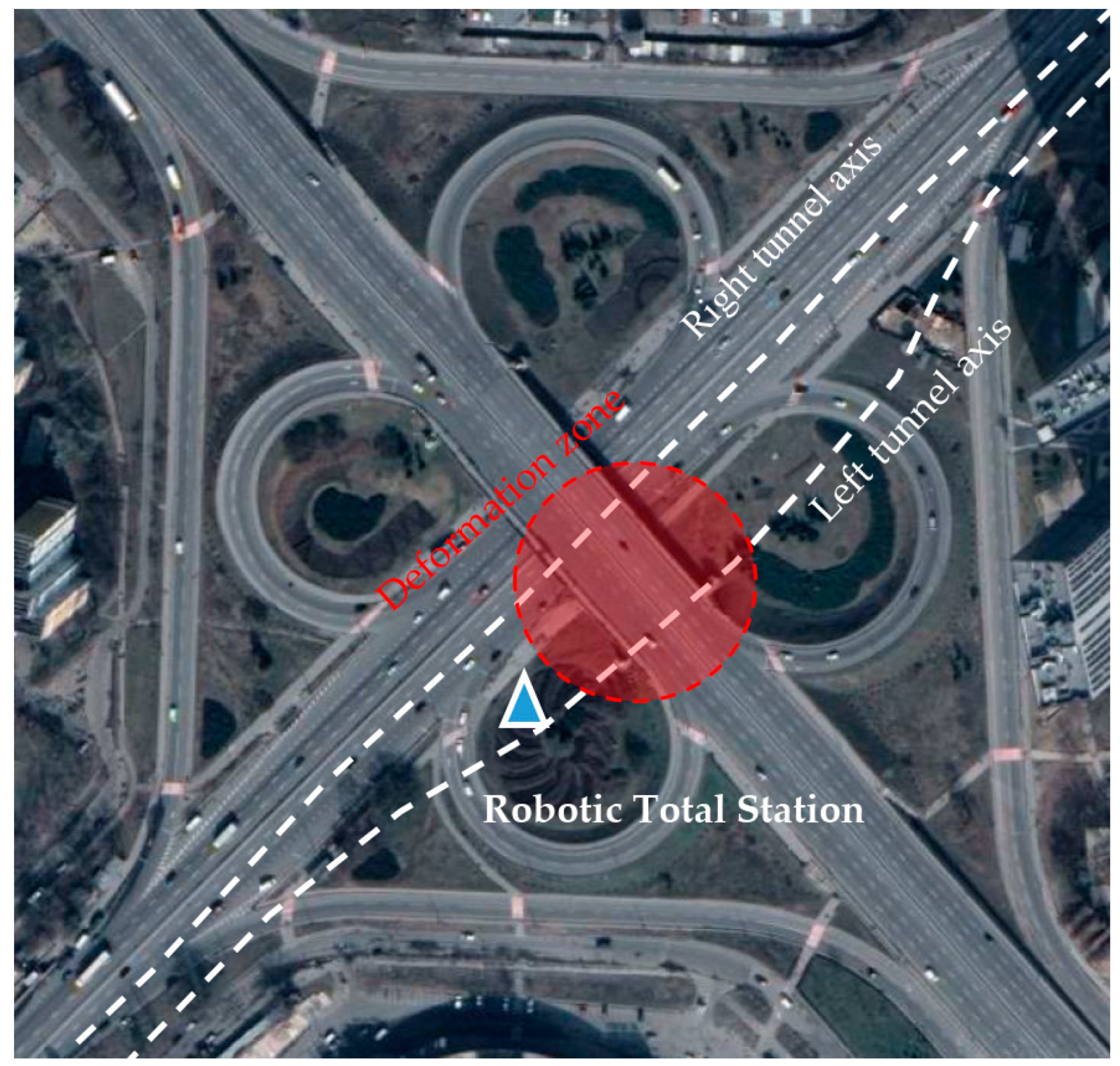
Figure 1. Cloverleaf interchange and the projections of the new tunnels’ axis.
Urbansci 07 00100 g001
Figure 2. Sketch of the overpass cross-section (non-scaled).
Urbansci 07 00100 g002
Figure 3. The ramp failure with land subsidence (left picture) and the cracks on the overpass surface (right picture).
Urbansci 07 00100 g003
Figure 4. Observation areas A and B.
Urbansci 07 00100 g004
Figure 5. Deformation targets on the pillars in area A.
Urbansci 07 00100 g005
Figure 6. Deformation targets underneath the overpass’s slab in area B.
Urbansci 07 00100 g006
Figure 7. Horizontal displacements along the X–axis for the deformation targets in area A (right tunnel).
Urbansci 07 00100 g007
Figure 8. Horizontal displacements along the Y–axis for the deformation targets in area A (right tunnel).
Urbansci 07 00100 g008
Figure 9. Vertical displacements along the Z–axis for the deformation targets in area A (right tunnel).
Urbansci 07 00100 g009
Figure 10. Horizontal displacements along the X–axis for the deformation targets in area B (left tunnel).
Urbansci 07 00100 g010
Figure 11. Horizontal displacements along the Y–axis for the deformation targets in area B (left tunnel).
Urbansci 07 00100 g011
Figure 12. Vertical displacements along the Z–axis for the deformation targets in area B (left tunnel).
Urbansci 07 00100 g012
Figure 13. Temperature and precipitation charts for the monitoring period.
Urbansci 07 00100 g013
Figure 14. The dependency between the subsidence coefficient and TBM position.
Urbansci 07 00100 g014
Figure 15. Machine learning flowchart.
Urbansci 07 00100 g015
Figure 16. Simulation metrics for the validation data, area A.
Urbansci 07 00100 g016
Figure 17. Simulation metrics for the validation data, area B.
Urbansci 07 00100 g017
Figure 18. Simulation metrics for the testing data, area A.
Urbansci 07 00100 g018
Figure 19. Simulation metrics for the testing data, area B.
Urbansci 07 00100 g019
Figure 20. Simulation metrics for the validation data, area A, root mean square error.
Urbansci 07 00100 g020
Figure 21. Simulation metrics for the validation data, area B, root mean square error.
Urbansci 07 00100 g021
Figure 22. Simulation metrics for the testing data, area A, root mean square error.
Urbansci 07 00100 g022
Figure 23. Simulation metrics for the testing data, area B, root mean square error.
Urbansci 07 00100 g023
Figure 24. Model performance for validation data subset, area A.
Urbansci 07 00100 g024
Figure 25. Model performance for testing data subset, area A.
Urbansci 07 00100 g025
Figure 26. Model performance for validation data subset, area B.
Urbansci 07 00100 g026
Figure 27. Model performance for testing data subset, area B.
Urbansci 07 00100 g027
Figure 28. Actual displacements and predicted displacements TB5X.
Urbansci 07 00100 g028
Figure 29. Correspondence between actual displacements and predicted displacements for validation data TB5X.
Urbansci 07 00100 g029
Figure 30. Correspondence between actual displacements and predicted displacements for testing data TB5X.
Urbansci 07 00100 g030
Figure 31. Residuals for the validation data subset TB5X.
Urbansci 07 00100 g031
Figure 32. Residuals for the testing data subset TB5X.
Urbansci 07 00100 g032
Figure 33. Importance scores for regression model parameters TB5X.
Urbansci 07 00100 g033
Figure 34. Model performance for validation data subset, area A.
Urbansci 07 00100 g034
Figure 35. Model performance for testing data subset, area A.
Urbansci 07 00100 g035
Figure 36. Model performance for validation data subset, area B.
Urbansci 07 00100 g036
Figure 37. Model performance for testing data subset, area B.
Urbansci 07 00100 g037
Figure 38. Actual displacements and predicted displacements TA6X.
Urbansci 07 00100 g038
Figure 39. Correspondence between actual displacements and predicted displacements for the validation data TA6X.
Urbansci 07 00100 g039
Figure 40. Correspondence between actual displacements and predicted displacements for the testing data TA6X.
Urbansci 07 00100 g040
Figure 41. Residuals for the validation data subset TA6X.
Urbansci 07 00100 g041
Figure 42. Residuals for the testing data subset TA6X.
Urbansci 07 00100 g042
Figure 43. Importance scores for neural network regression model parameters.
Urbansci 07 00100 g043
Figure 44. MSE graphs for optimizable neural networks for the deformation target TB8Z.
Urbansci 07 00100 g044
Figure 45. Determined and predicted displacements for the optimizable neural network regression for the deformation target TB8Z.
Urbansci 07 00100 g045
Table 1. List of the trained neural network models.
ModelActivation FunctionNumber of LayersNumber of Outputs in Each Layer
Model 1Rectified linear unit110
Model 2210, 10
Model 3310, 10, 10
Model 4330, 20, 10
Model 5120
Model 6150
Model 7Hyperbolic tangent110
Model 8210, 10
Model 9310, 10, 10
Model 10330, 20, 10
Model 11120
Model 12150
Model 13Sigmoid function110
Model 14210, 10
Model 15310, 10, 10
Model 16330, 20, 10
Model 17120
Model 18150
Model 19Identity function110
Model 20210, 10
Model 21310, 10, 10
Model 22330, 20, 10
Model 23120
Model 24150
Table 2. Model performance for validation, area A, regression analysis.
TargetValidationTesting
TA1XStepwise Linear RegressionLinear Regression Quadratic
TA2XStepwise Linear RegressionLinear Regression Quadratic
TA3XStepwise Linear RegressionLinear Regression Quadratic
TA4XFF
TA5XFF
TA6XFF
TA1YStepwise Linear RegressionLinear Regression Quadratic
TA2YFF
TA3YFF
TA4YFF
TA5YFF
TA6YFF
TA1ZStepwise Linear RegressionStepwise Linear Regression
TA2ZFLinear Regression Quadratic
TA3ZFLinear Regression Quadratic
TA4ZFF
TA5ZStepwise Linear RegressionF
TA6ZFF
Table 3. Model performance for validation, area B, regression analysis.
TargetValidationTesting
TB1XStepwise Linear RegressionLinear Regression Quadratic
TB2XStepwise Linear RegressionF
TB3XStepwise Linear RegressionLinear Regression Quadratic
TB4XLinear RegressionLinear Regression Quadratic
TB5XStepwise Linear RegressionStepwise Linear Regression
TB6XStepwise Linear RegressionLinear Regression Quadratic
TB7XStepwise Linear RegressionF
TB8XStepwise Linear RegressionLinear Regression Robust
TB9XFF
TB1YFF
TB2YFF
TB3YStepwise Linear RegressionLinear Regression Quadratic
TB4YFF
TB5YStepwise Linear RegressionStepwise Linear Regression
TB6YStepwise Linear RegressionLinear Regression Quadratic
TB7YFLinear Regression Quadratic
TB8YStepwise Linear RegressionLinear Regression Quadratic
TB9YStepwise Linear RegressionF
TB1ZStepwise Linear RegressionF
TB2ZStepwise Linear RegressionF
TB3ZFF
TB4ZFStepwise Linear Regression
TB5ZFStepwise Linear Regression
TB6ZFF
TB7ZStepwise Linear RegressionF
TB8ZFStepwise Linear Regression
TB9ZFF
Table 4. Model performance for testing, area A, neural network regression.
TargetValidationTesting
TA1XModel 17Model 7, 11, 12
TA2XModel 9,10Model 6
TA3XModel 9, 10, 14Model 17, 18
TA4XModel 14Model 10
TA5XModel 16Model 8
TA6XModel 16Model 8
TA1YModel 9, 10Model 9, 10
TA2YModel 9, 10Model 9, 10
TA3YFF
TA4YModel 9Model 9
TA5YModel 9Model 16
TA6YModel 10Model 16
TA1ZModel 10Model 16
TA2ZModel 10Model 2, 13
TA3ZModel 10Model 2, 7, 13
TA4ZModel 10Model 16
TA5ZModel 10Model 9
TA6ZModel 10Model 9
Table 5. Model performance for testing, area B, neural network regression.
TargetValidationTesting
TB1XModel 16Model 3
TB2XModel 22Model 3
TB3XModel 18, 21, 22Model 19
TB4XModel 5Model 16
TB5XModel 22F
TB6XFModel 24
TB7XModel 6F
TB8XFF
TB9XFF
TB1YFModel 16
TB2YModel 8Model 4
TB3YModel 18Model 10, 12
TB4YModel 7F
TB5YModel 7F
TB6YModel 11, 14Model 10
TB7YModel 11, 13Model 12
TB8YModel 11, 13Model 12
TB9YModel 7, 13, 18Model 16
TB1ZModel 16Model 4
TB2ZModel 13Model 3, 10
TB3ZModel 10, 16Model 9, 16
TB4ZModel 15F
TB5ZModel 10Model 10
TB6ZModel 10Model 10
TB7ZModel 16Model 16
TB8ZFF
TB9ZFF
Table 6. Hyperparameters for optimizable neural network regression for the deformation target TB8Z.
Layer 1Layer 2Layer 3Activation FunctionMSEValidation RMSE, mmValidation R-SquareTesting RMSE, mmTesting R-Square
1268Hyperbolic tangent0.560.750.770.780.72
1300-Hyperbolic tangent0.630.740.770.800.70
1446Sigmoid0.590.760.760.790.71
2--Sigmoid0.600.780.750.710.76
Disclaimer/Publisher’s Note: The statements, opinions and data contained in all publications are solely those of the individual author(s) and contributor(s) and not of MDPI and/or the editor(s). MDPI and/or the editor(s) disclaim responsibility for any injury to people or property resulting from any ideas, methods, instructions or products referred to in the content.