Towards a Model of Urban Evolution: Part II: Formal Model

Abstract

This paper is part II of “Towards A Model of Urban Evolution.” It defines a formal model of the Signature of an urban space, comprised of the information encoded in that space. This information consists of: an urban genome, which captures ideas regarding the groups (i.e., users) and activities (i.e., uses) to which a space’s physical forms are oriented; ideas among human actors regarding who (users) and how (uses) to utilize the space and its forms; and the signals that are communicated within and among urban spaces. Central to the model is the notion of the formeme, which provides the building blocks for a Signature. Formemes are units of urban information regarding physical forms, groups, and activities, which may be encoded in physical artifacts, signals, or human actors, and circulate among them. We then show how various metrics can define an urban area based on its Signature, and that these metrics can be used to measure similarity of urban spaces. The Signature, and its underlying formemes capture the sources of variations in urban evolution.

1. Introduction

In Part I of “Towards of Model of Urban Evolution” [1] we reviewed the literature related to urban evolution from the perspectives of urban theory and socio-cultural evolution. Taking our cue from the sociocultural evolution literature, we start from the proposition that the units of urban evolution are themselves sociocultural entities, such as buildings, roads, parks, neighborhood types, porches, building codes, city plans, zoning regulations, and the like. While this might seem like a “physicalist” orientation, we also follow the sociocultural evolution literature in proposing that these entities embody “iss and oughts”. They are evolved responses to problems about how to organize space, not only in terms of physical design, but also in terms of who and what the space is for, that is, in terms of its characteristic groups and activities [2]. Therefore, the basic units of urban evolution should encode information about how a space is physically organized, and who and what it is for.

We proposed a “formeme” as the basic unit of evolution. A set of formemes consists of specific information about how to organize urban space as a combination of physical features and the groups and activities toward which they are oriented. Formemes are ideas or information for physically organizing space for some sets of activities and groups. This definition might also be summarized as a script or set of instructions: “be made out of this stuff arranged in this way, for doing these things for groups of people like this”. The cities we observe are encoded with large populations of such scripts. The complete set of scripts encoded in a given place may be defined as its urban genome—which is itself a set of formemes. These formemes admit of variations, some of which are selected and retained. Variation, selection, and retention produce evolution, both in the sense of adaptation to local environments and the generation of historical lineages and trajectories characterized by shared, derived characteristics.

In this paper, Part II, we define a formal, mathematical model for encoding the key characteristics of an urban space as formemes. A central task of the formal model is to rigorously elaborate the intuitions behind the concepts of formeme and urban genome, and their role in the evolutionary algorithm of variation-selection-retention. Brown [3] illustrates this general approach to formalization and theory construction in the social sciences with the example of Simon’s [4] reconstruction of Homans’ exchange model. The value of such formalization comes in part in revealing the logical skeleton of informal models, but even more in identifying their key assumptions and omissions, as well as necessary auxiliaries and correctives. In the ideal case, formalization will make evident new connections and implications, and produce an “idealized” model against which empirical phenomena can be measured (At the same time, committing to a particular formalism may inhibit or exclude possibly relevant characteristics of a spatial area). Part III of this series of papers [5] demonstrates how this formalization of the formeme can be used to encode the evolutionary processes of variation, selection and retention. Part IV in this series [6] then applies our formalization to Yelp data and demonstrates how the encoding can be used to measure both longitudinal and transversal formetic distance.

In the following we first define the components of our model which are composed of spatial areas, physical forms, activities, and groups. We then introduce the concept of a formeme and show how it is modelled using these components. Using formemes as our basic building block, we introduce a spatial area’s signature which represents a spatial area’s formetic description at some point in time. This description captures the urban genome, human uses and users, and signals. With our model defined, we then define various metrics that can be applied to the model, and show how they can be used to measure the similarity of signatures. We finish with a discussion of questions that our model raises.

2. Basic Model

Our goal in this Part is to create a formal model that includes basic constituents of the urban evolutionary process, and provides a rich expressive language that can be applied and extended further.

2.1. Components

At the core of the model is the spatial area that is being modelled.

C: the set of all spatial areas in the domain.

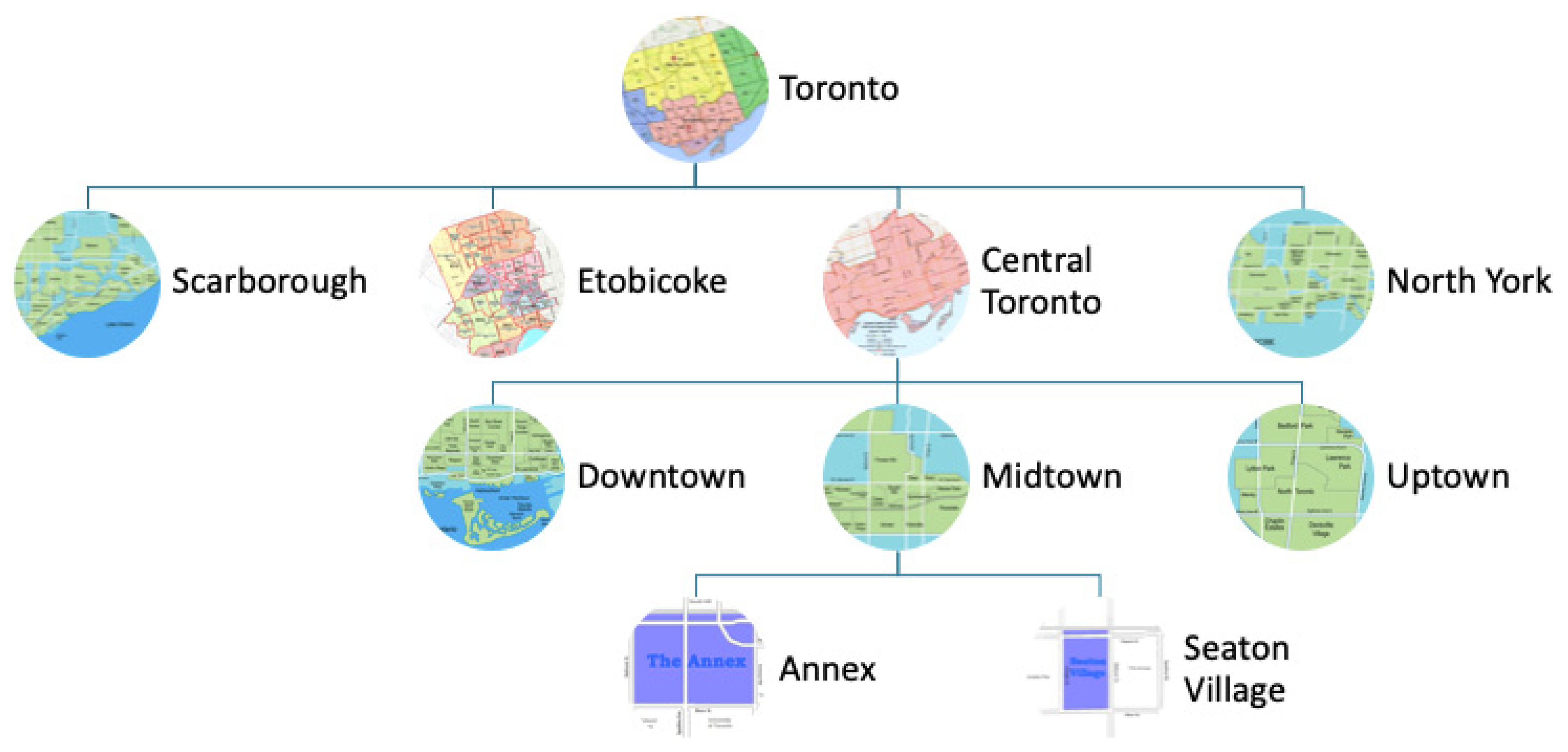
Members of C can be spatially related using standard geo-spatial or administrative primitives. We denote that spatial area c2 is contained within or equal to spatial area c1 by: c2 ⊆ c1. A model can be created for any member of C, allowing for the modelling of an urban area at different levels of aggregation and alternative spatial boundaries. Figure 1 depicts a hierarchical structuring of the members of C for the City of Toronto. We can model the City at varying levels of spatial or administrative aggregation.

Our model of a spatial area c is comprised of three “components”:

P:	the set of all possible types of physical Forms.
A:	the set of all possible types of Activities (uses).
G:	the set of all possible types of Groups (users).

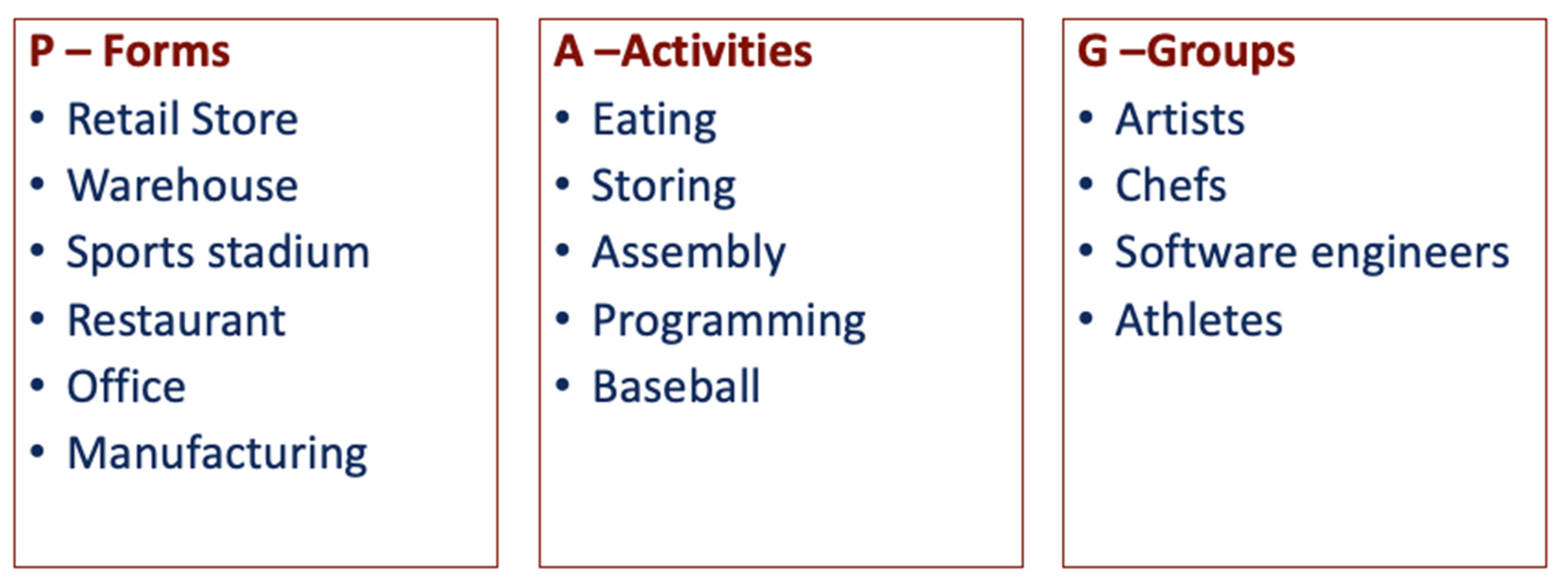
Any member of a component is referred to as an element (e). For example (Figure 2), a warehouse is an element of the component P. The elements of each component determine how expressive the model will be. For example, if “vehicle” is an element of P, but it does not include any types of vehicles, then the model cannot differentiate among different types of vehicles. On the other hand if “bus”, “subway”, “car”, and “truck” are elements of P, then the model can support a more nuanced representation and analysis of an urban area. By restricting the elements within a component, the nature of the analysis is in turn restricted. For example, one could restrict the components to focusing solely on eating, including restaurants and groceries, and the groups of people and activities associated with them.

2.2. Formeme

Central to our model is the recognition that P, A and G are interdependent. Forms enable activities performed by groups. However, the relationship is not uni-directional. Groups impose their own interpretation of forms in order to carry out activities for which the forms may not have been designed. This makes the forms subject to evolutionary processes, as new uses accumulate upon or transform the old.

To capture the relationship among elements of P, A and G, we introduce the concept of formeme. Formemes are units of information regarding the organization of urban space, enabling features of urban space to be replicated elsewhere, maintained into the future, or recoded into new configurations. The formeme concept extends the concept of the “meme” to the urban domain. “Memes” are, in simple terms, “ideas that spread” or “information worth copying” (A somewhat fuller definition would be: “information such as knowledge, beliefs, and values that is inherited through social learning and expressed in behavior and artifacts” [7]. While the meme concept has been subjected to recurrent critique, we find it valuable in our research context, even as we have no fundamental commitment to any particular term. The concept is valuable in that it allows us to model the flow of urban information among agents, physical space, and signals, and the changes such information undergoes as it becomes encoded in various forms. Part I of this series discusses the concept in more detail, and points to relevant literature and debates. The “meme” in “formeme” highlights that information regarding urban form can be copied and retained—formemes are “free-floating rationales” [8] for how to organize space, which can be picked up and applied elsewhere. Formemes can be encoded in artifacts and institutions (such as buildings, street grids, housing types, zoning rules), the minds and habits of human actors, and communication media (such as books, webpages, or photographs). If one space is programmed to “be made out of this stuff, for these people, doing these things,” another can as well—to some degree of fidelity, via some mechanisms of communication and inheritance (the exact degree and process is an empirical question, and will affect the nature of the evolutionary sequences that follow). For example, the cul-de-sac was deployed in English Garden City designs at the beginning of the twentieth century, and then appeared in many areas thereafter; it embodied an urban idea that spread. The cul-de-sac encoded a relatively successful formeme, both in terms of how far it has spread and the fidelity of its copies.

A formeme f is defined to be a triple composed of P, A and G.

f = <f[p], f[a], f[g]> where f[p] ⊆ P ∧ f[g] ⊆ G ∧ f[a] ⊆ A

f[p] can be understood as an idea about how to organize the physical design of a space, which we might summarize “be made out of this stuff arranged in this way.” For a building, a very crude characterization of f[p] could refer to being made out of brick and steel with long-span floor spaces. The more areas that are programmed in this way, the more prevalent this variant of f[p] has become.

These sorts of physical properties are not the only information encoded in an area. It is programmed for somebody to do something. A very similar physical space made out of brick and steel could be for shipping and receiving by employees with certain occupational credentials or for late-night entertainment venue by dancing enthusiasts. Our model seeks to capture this additional information with the terms f[a] and f[g]. f[a] and f[g] can be understood as ways of coding space in terms of what and who it is for: “be a place for doing these things f[a] for groups of people like this (f[g])”. f[a] and f[g] can be manifest in a number of ways. This information may be explicit, in a zoning designation (for industrial or entertainment), a sign on the wall (“only employees may enter”), or a dress code and drink minimum. The information may also be implicit, in an array of signs and cues that indicate who is and is not supposed to be there, and what they should and should not be doing. These are the “iss and oughts” of urban life.

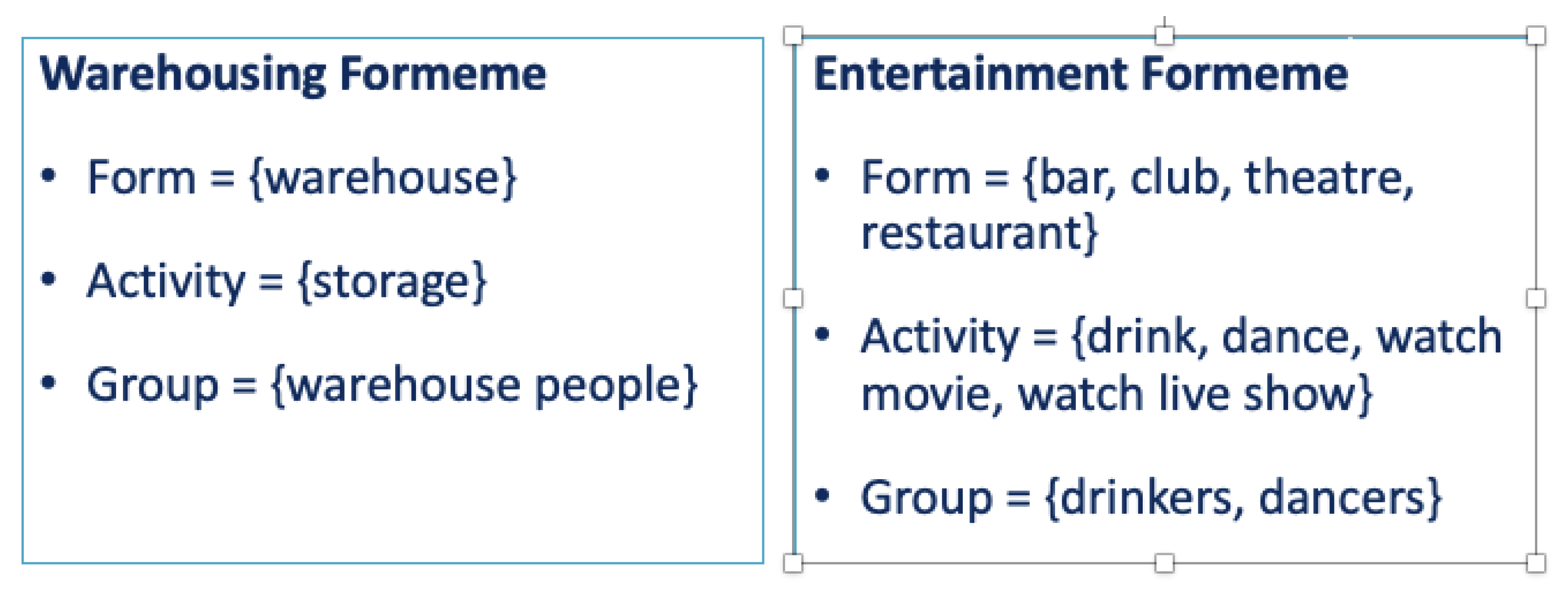
Figure 3 depicts two example formemes: a Warehousing formeme where there is a single element for each component, and Entertainment formeme where there are several elements for each component. Note that elements can be defined at any level of abstraction or aggregation as required for the modelling task. For example, “entertainment venue” could be substituted for “bar, club, theatre, restaurant” in the Entertainment formeme Form.

We define the predicate Formeme to denote that a particular f is a formeme:

Formeme(f) is true if f[p] ⊆ P ∧ f[g] ⊆ G ∧ f[a] ⊆ A

$\mathcal{F}$: the powerset of all possible formemes, i.e., combinations of P, G and A

= {<p, g, a> | p ⊆ P ∧ g ⊆ G ∧ a ⊆ A}

We define the predicate SubFormeme which is true if one formeme is a subset of another:

SubFormeme(f, f’) = f[p] ⊆ f’[p] ∧ f[g] ⊆ f’[g] ∧ f[a] ⊆ f’[a]

Finally, we define a primitive formeme as a formeme that has at most one element for each of f[p], f[g] and f[a].

primFormeme(f) = True iff |f[p]| ≤ 1 ∧ |f[g]| ≤ 1 ∧ |f[a]| ≤ 1

2.3. Genome

The Genome of a spatial area captures the set of formemes encoded in a given area at a given time. It codifies the evolution of a spatial area at some time t. It defines the way an area is programmed in terms of how it is physically organized, the activities to be performed there, and the groups who are to perform them.

We define a genome U as a set of formemes:

U = { u | Formeme(u) }

Expressed another way, U is a subset of the powerset of formemes: U ⊆ $\mathcal{F}$

We define

ui:	the ith formeme in U
ui [p]:	the set of forms in the ith formeme in U
ui [a]:	the set of activities in the ith formeme in U
ui [g]:	the set of groups in the ith formeme in U

and

U[p] = ⊔_i u_i[p], set of all forms in U

U[a] = ⊔_i u_i[a], set of all activities in U

U[g] = ⊔_i u_i[g], set of all groups in U

Figure 4 depicts two examples of genomes. The first genome describes a light industrial zone composed of three formemes. u1 describes warehousing usage, u2 describes manufacturing usage, and u3 describes service usage. All three co-occur within the same spatial area. The second genome is also composed of 3 formemes describing entertainment related forms, users and activities, all existing/occurring in the same spatial area. In Figure 4, the genomes labeled “light industrial zone” and “entertainment zone” can be interpreted as land use where their formemes specify the forms and associated activities and groups. In this context, the word “warehouse” may be taken as a shorthand for the physical composition and arrangement of the structures in that location.

We define the Urban Genome as tying a specific genome U to a spatial location c, at time t:

Genome(c, t, U, w) where

     c: denotes a spatial area

          t: denotes the time at which the genome describes c

          w: denotes the world in which U exists.

In most cases, we will omit w, but when we need to compare alternative scenarios for the same space c and time t, w will be used to distinguish them (i.e., alternative worlds).

In this document we use the function UG to denote the genome for a specific spatial area c and time t:

UG(c, t) = U = { u | Formeme(u) } for a space c at time t

in other words c and t uniquely identify a specific genome.

2.4. Users, Uses and Used

The genome describes the way a space is programmed physically and for certain uses and users. Local human actors, however, may nor may not share this conception. If they do, they are likely to maintain it and carry it with them elsewhere; if they do not, they may reprogram the area in the light of their own ideas about how to organize urban space.

Hence, we define the Hunome H: the set of formemes encoded in the minds, habits, or routines of human actors. This introduces the beginning of a dynamic component to the model, representing the process by which formemes circulate among and compete for priority in urban space and human minds. This dynamism will be crucial for a model of urban evolution, as it is a central source of novel variations, their differential reproduction, and their degrees of retention.

We define H as a set of formemes. Just like the urban genome U, formemes are also the primitive “material” used to construct H, as each is defined by information regarding physical forms, activities, and groups. Where U is the formetic information encoded in an area’s physical forms, H is the formetic information encoded in its human users’ customs, practices, routines, and modes of interpretation. U is information regarding what the space expects from its users; H is information regarding what the people expect from their spaces.

Formally, we define the Hunome H as:

H = { h | Formeme(h) }

Expressed another way, H is a subset of the powerset of formemes: H ⊆ $\mathcal{F}$

We define

hi:	the ith formeme in H
hi [p]:	the set of physical forms in the ith formeme in H
hi [a]:	the set of activities in the ith formeme in H
hi [g]:	the set of groups in the ith formeme in H

and

    H[p] = ⊔_i h_i[p],  set of all forms in H

    H[a] = ⊔_i h_i[a],  set of all activities in H

    H[g] = ⊔_i h_i[g],  set of all groups in H

In this document we use the function HG to denote the Hunome for a specific spatial area c and time t:

HG(c, t) = H = { h_i | Formeme(h_i) } that exist for some space c at time t

Figure 5 represents local actors who frequent a light industrial zone. Some local actors regard the space (h1) as a warehouse suitable for storage activities or (h2) light manufacturing. Others regard it as suitable for dancing by hipsters (h3). This formeme co-exists with those found in other users of the area, and may or may not come to define how it is organized (e.g., it may or may not become encoded in genome G).

2.5. Signal

Signals are crucial features of an urban evolutionary model. Any code must be communicated via some mechanism and we call that mechanism the Signal (S). Potential users can access the relevant urban information encoded in the genome only if that information can be transmitted to them via a method they can interpret. Characteristics invisible to potential users are unlikely to survive, while those that reach a broad audience may have a better chance of recruiting users and being replicated elsewhere.

The concept of Signals makes it possible to incorporate the environment into our model. The environment is a crucial concept for any evolutionary model. We conceptualize the environment as the communicative context in which a given spatial area exists; it is the set of formemes that a given area receives via Signals of any type. This generic communicative environment becomes an institutional environment when the surrounding signals carry with them a sanction (This is a fairly minimalist conception of institutions that largely comports with standard notions in sociological theory and the philosophy of social science [9], which tend to highlight institutions as a combination of roles and sanctions held together by communicative media). A sanction is a penalty or cost for deviating from the message contained in the Signal. For example, a spatial area within a city receives signals from City Hall in the form of by-laws, which raise the cost of renovating buildings in ways that do not accord with the formemes expressed in the by-law. A spatial area that does not receive this Signal by contrast would have lower recoding costs with respect to the same formemes, and would accordingly exist largely outside the institutional reach of City Hall. We conceptualize sanction as recoding costs.

The conceptualization of the concepts of the environment and institutions is an important illustration of the analytical power of our model’s formal language. It shows how the model can explain higher order concepts by reducing them to analytical elements and functions. This in turn makes highly abstract notions like “environment” and “institution” more empirically and theoretically tractable.

We define S to be a set of signals received and processed within the spatial area c, where each signal is composed of a:

• formeme that communicates a fragment of a genome. This fragment may be assimilated by another spatial area, first as a change to hunome H, and if it survives, eventually as a change to U;
• the source of the signal a spatial area receives. Where a signal comes from affects how it is received;
• method of communication. A formeme may be communicated in more than one way, and depending on the method of communication, the signal may travel only within c (intra-spatial signal), or between c’s (inter-spatial signal), or both (bi-spatial signal);
• the capacity of a signal to alter the recoding costs in the area that receives the signal; and
• the number of times the signal has been received. A signal that is received with a high frequency may have a higher probability of assimilation in H.

S = { s_i | s_i = <f, r, c, sf, cm, n> }

where

f is a formeme that is being signaled

r is a function that transforms the recoding cost function R in the receiving signature

c is a spatial area from which the signal originates

sf is a set of formemes that is the source of the signal in c

cm is the set of communication methods

n is the number of times s_i has been received from c during the time span of the signature

We define:

s_i: the i^th signal in S

s_i[f]: is the formeme f of the i^th signal

s_i[r]: is the recoding cost transform

s_i[c]: is the spatial area from which the signal originates

s_i[sf]: is the formeme sf that is the source of the i^th signal

s_i[cm]: is the communication methods of the i^th signal

s_i,[n]: is the frequency of the i^th signal from c during the time span of the signature

and

   S[p] = ⊔_i s_i[f][p]  set of all forms in S

   S[a] = ⊔_i s_i[f][a]  set of all activities in S

   S[g] = ⊔_i s_i[f][g] set of all groups in S

   S[f] = ⊔_i s_i[f]  set of all formemes in S

In this document we use the function SG to denote the Signal for a specific spatial area c and time t:

SG(c, t) = S = { s_i | Signal(s_i) } that exist for some space c at time t

A Valid Signal s_i satisfies the following requirements:

• Formeme Validity: Formeme (s_i[f]) is true.
• Source Validity: Given the source spatial area c and formeme s_i[sf], then s_i[sf] ∈ UG(c,t)
• Signal Method Validity: s_i[cm] ⊆ CM (where CM is the set of all methods)

For a dance club, signal methods could include informal word of mouth chatter about what is happening Friday night, but also advertising and social media. For example, a Yelp review page tells potential users what is there, transmits information about what kind of ambiance to expect, price, location, typical users, and directs one to other websites to find out what is happening and when. For a roadway, radio traffic reports or apps such as Google Maps or Waze could be signals. The sign on the dance club therefore has two parts: the physical form which is a constituent of the club’s f[p] and the signal projected within or from this form.

The model also represents methods of communication used (or not) within a spatial area c, which may not be those used in signals to other areas. For example, China bans the use of Google services within its boundaries, but may use it in signals to other countries.

An illustration of the role of signalling in urban evolution is the proliferation of coffee shops in Seoul, South Korea. We can imagine that the growth of coffee chains in North America, such as Starbucks, led to signals containing the formeme:

f[p] = coffee shop design

f[a] = drinking coffee, socializing

f[g]= GenX, Millenials

Assuming a method of transmission such as Korean tourists visiting North America, discovering/enjoying Starbucks, or viewing videos of café culture, and returning home with this formeme in their minds, the signal directly impacts hunome H by changing the attitude toward activities (i.e., drinking coffee, socializing) of the relevant groups (ie., younger Korean urbanites). This results in the construction of coffee shops whose design is based on the formemes transmitted via the signal. Over time, these coffee shops will modify the genome for the area c they appear in.

Inter-spatial signals not only represent formemes from other spatial locations, but they can represent the broader spatial area of which the recipient of the signal is a part. This wider signal is a way to represent the surrounding environment as the messages locals receive from the broader context in which they are situated. For example, the city, state and country act as a source of environmental signals for a neighbourhood that is embedded in them. This signal environment may have a significant impact on the formemes that thrive in the hunome H, affecting the evolutionary path of the formemes in the genome U.

This environment is constituted generally by very abstract ideas about how to organize space, which can be embedded in cultural, political, and natural systems. For instance, broad cultural values concerning gender relations inform models of how to design houses and public spaces. Ancient Greek cities were laid out to emphasize democratic egalitarianism. Religious concepts have similarly structured the arrangement of space, for instance in palatial centers or how the position of Arabic-Islamic cities was designed using the Fiqh paradigm, which was an attempt to express religious principles through urban form [10]. Similarly, rules, laws and policies can be encoded as formemes and signalled by an enclosing spatial area, e.g., state, to an enclosed spatial area, e.g., city.

The environment will often exert selection pressures upon people within it, which will in turn affect the probability of a given lower-order formeme or genome propagating there. This occurs through the recoding cost transformation function carried in signals. For example, a building code communicated from the state capitol transforms the recoding costs for the spatial areas within that state. It raises the cost of building something that does not conform to the code, and communicates this function by way of groups such as building inspectors. As the recoding cost transformation function becomes more effective at altering the local recoding costs, the signal environment becomes the predominant site for evolutionary changes. Changes to a building becomes less likely to survive unless they become encoded in the signal. In other words, a new style will be an evolutionary dead-end unless it becomes embedded in the relevant laws, policies, and norms. However, the reverse is possible: lower order formemes can engender a surrounding environment conducive to their own success. This is an urban variant of niche formation.

2.6. Signature

To complete the definition of the basic terms in our model, we introduce the notion of a Signature. The signature combines the aforementioned concepts to provide a complete representation of a spatial area at some time t. It tells us the set of formemes encoded in the space, i.e., the genome U, the formemes informing its users, the hunome H, and the formemes transmitted there via signals, S. In addition, a Signature includes a recoding cost function R which captures the cost of recoding/transforming a formeme into another. R is defined in Section 8. The function R is necessary for a complete analysis of environment and institutions as outlined above.

Signature(c, t, U, H, S, R, w)

We can now define the function:

SIG(c, t, w) = <U, H, S, R>

in other words, the complete signature for space c at time t.

Note that the ordering of formemes within the Genome or Humome is immaterial. What is material is the location of a signature in both time and space enabling longitudinal and transversal analysis of urban genome evolution.

3. Component Characteristics

Any element can have zero or more attributes. For example, the number of the same elements, e.g., the number of restaurants, eating activities, and chefs, may be an important characteristic of a spatial area. Since, the size or number of a type of element is important, we define three functions that return the quantity of instances of e at spatial location c at time t, where e ∈ P ∪ A ∪ G. If e is an activity, it can represent the number of occurrences of that activity up to time t. If e is a group, it can represent the number of people in the group at time t.

Usize(c, t, e):	is the number of times e appears in formemes in the genome,
	i.e., e ∈ U.
Hsize(c, t, e):	is the number of times e appears in formemes in the hunome,
	i.e., e ∈ H.
Fsize(F, e):	is the number of times e appear in a set of formemes F.

Another attribute of interest is the value (e.g., monetary value) associated with an element. For example, the value of a building, parcel of land, the assets of a group, or perhaps value associated with the ability to perform an activity. We define:

value(c, t, e):	is a function that returns the value of e at spatial location c
	at time t where e ∈ P ∪ A ∪ G.

• Signal characteristics

Signals may vary in the impact on changing the formemes in a Signature. In this section we focus on measuring the characteristics of S that lead to variations in impact.

Signal Reach. The characteristic reach refers to the percentage of the population that is able to receive and process signal s within c at time t.

reach(s, c, t):	% of population within c at time t that receive and can process
	the signal.

Not all signals reach the target population within c. Not everyone follows twitter, or has a facebook page. Marketing emails have a notoriously low percentage that are actually opened. While electronic communications may have great speed, and cover large distances, their reach may be minimal. Similarly, the reach across spatial areas will differ. Some areas are more attuned to social media than others, leading to differences in reach. This naturally leads to further differentiation of reach by group:

reachG(s, c, t, g):	% of a group g within spatial area c at time t that receive
	the signal.

Signal Audience and Precision. Signals have a target audience. This is the groups within c for whom they are targeted.

audienceG(s, c, t, g):	predicate that denotes the signal s has a target
	audience of group g at time t

Precision refers to the percentage of audience that receive and processes the signal.

precisionG(s, c, t, g):	the percentage of group g in spatial area c at time t that
	is able to process the signal.

While a signal may have a large reach, its precision can be low as it may not be reaching the audience to which it is directed. Consider a by-law that prohibits BBQs at parks that is posted at each park versus one that only appears in the municipality’s records. The former has greater reach than the latter, assuming that municipal records are seen by very few residents. On the other hand, a general sign at the park that prohibits the use of flammable devices versus BBQs, will have lower precision than the latter, as some people may not interpret a flammable device as including a BBQ.

Signal Clarity. The characteristic clarity refers to the probability that the receiving group will correctly interpret the content of the signal.

clarityG(s, c, t, g):	probability that the recipient group g will correctly interpret
	the content of the signal s in spatial area c at time t.

Consider the BBQ bylaw again. A sign posted at a park stating “no fires” is less clear than a sign that states “no fires, including BBQs”.

Signal Noise. The characteristic noise refers to the degradation of the signal over distance and/or time (In classical Shannonian information theory, a signal can vary in two main ways, noise and cost. Noise refers to anything that interferes with and degrades a signal, and cost refers to difficulties in encoding and decoding information that reduce transmission speed). In particular, if signal s conveys a formeme f, then noise mutates f into f’.

noise(s, c1, t1, c2, t2):	percentage of the signal s content that mutates in
	transmission from spatial area c1 at time t1 to spatial
	area c2 at time t2.

How to compute the percentage of noise is an open question. One approach is to determine the % of the transmitted portion of f that is changed. This assumes some type of encoding where differences can be computed.

Signal noise and clarity introduces another dynamic element to the framework, because it allows for the strategic deployment of signals by actors who wish to misdirect or jam signals. Indeed, opportunistic actors can appropriate signals and misdirect them from their ‘natural’ state, potentially shifting survival rates of affected formemes.

Signal Frequency. The frequency with which information about a formeme is received can determine its effect on the formemes incorporated into local human agents hunome H; more frequent signals may have a higher probability of altering H. We first have to know what signals are received by the spatial area. We define receivedSignals as the set of signals received by a spatial area c during the time interval [t, t’]:

receivedSignals(c, t, t’) is the set of signals received by location c between t and t’

and the signals sent by a spatial area c during time interval [t, t’]:

sentSignals(c, t, t’) is the set of signals sent by location c between t and t’

We can define the frequency of a formeme found in receivedSignals:

$$\mathrm{formemeSignalFrequency}\left(\mathrm{c}, \mathrm{t}, \mathrm{t}’, \mathrm{f}’\right)=\frac{| \{ \mathrm{s} | \mathrm{s} \in \mathrm{receivedSignals}\left(\mathrm{c}, \mathrm{t}, \mathrm{t}’\right) \wedge \mathrm{SubFormeme}\left(\mathrm{f}’, \mathrm{s}\left[\mathrm{f}\right] \right) \} |}{\left| \mathrm{receivedSignals}\left(\mathrm{c}, \mathrm{t}, \mathrm{t}’\right)\right|}$$

where s[f] are the formemes of signal s.

Similarly we can define the frequency of a formeme in sent signals:

formemeSentSignalFrequency(c,t,t’,f’) = | { s | s ∈ sentSignals(c, t, t’) ∧ SubFormeme(f’, s[f] ) } |

where s[f] are the formemes of signal s.

4. Similarity and Formetic Distance

An important concept in modelling urban evolution is the degree to which formemes are similar. By similarity, we mean the degree to which they share the same elements: forms, activities, and groups. The hypothesis is the more similar the formemes, the more similar the evolutionary path of the genome. However, if similar genomes diverge over time, what are the key differences in formeme elements that lead to the change?

We introduce the function fdist that returns the formetic distance between two formemes.

fdist(f1, f2): measures the formetic distance between formemes f1 and f2.

The smaller the value, the more similar the formemes are. There can be many different distance metrics. fdist() is minimally ordinal. We constrain the definition of fdist as follows:

Axiom 1:	Reflexivity fdist(f1, f1) = 0
Axiom 2:	Symmetry fdist(f1, f2) = fdist(f2, f1)
Axiom 3:	Subadditivity fdist(f1, f2) + fdist(f2, f3) ≥ fdist(f1, f3)

One possible definition is bfdist, which is based on the total number of elements common to both formemes, divided by the total number of unique elements:

$$\mathrm{bfdist}\left(\mathrm{f}1, \mathrm{f}2\right)=1-\frac{\left| \mathrm{f}1\left[\mathrm{p}\right] \cap \mathrm{f}2\left[\mathrm{p}\right] \left|+\right| \mathrm{f}1\left[\mathrm{a}\right] \cap \mathrm{f}2\left[\mathrm{a}\right] \left|+\right| \mathrm{f}1\left[\mathrm{g}\right] \cap \mathrm{f}2\left[\mathrm{g}\right] \right|}{\left| \mathrm{f}1\left[\mathrm{p}\right] \cap \mathrm{f}2\left[\mathrm{p}\right] \left|+\right| \mathrm{f}1\left[\mathrm{a}\right] \cap \mathrm{f}2\left[\mathrm{a}\right] \left|+\right| \mathrm{f}1\left[\mathrm{g}\right] \cap \mathrm{f}2\left[\mathrm{g}\right]\right|}$$

In order to measure how similar urban genomes are, we define the distance between two sets of Formemes F1 and F2:

Fdist(F1, F2): measures the formetic distance between formeme sets F1 and F2.

The smaller the value, the more similar the formeme sets are. There can be many different distance metrics. Fdist() is minimally ordinal. We constrain the definition of Fdist() as follows:

Axiom 1:	Reflexivity Fdist (F1, F1) = 0
Axiom 2:	Symmetry Fdist (F1, F2) = Fdist (F2, F1)
Axiom 3:	Subadditivity Fdist (F1, F2) + Fdist (F2, F3) ≥ Fdist (F1, F3)

One possible definition is bFdist(), which counts the number of element types shared between the formeme sets divided by the total number of element types across both formeme sets.

$$\mathrm{bFdist}\left(\mathrm{F}1, \mathrm{F}2\right)=1-\frac{\left| \mathrm{F}1\left[\mathrm{p}\right] \cap \mathrm{F}2\left[\mathrm{p}\right] \left|+\right| \mathrm{F}1\left[\mathrm{a}\right] \cap \mathrm{F}2\left[\mathrm{a}\right] \left|+\right| \mathrm{F}1\left[\mathrm{g}\right] \cap \mathrm{F}2\left[\mathrm{g}\right] \right|}{\left| \mathrm{F}1\left[\mathrm{p}\right] \cap \mathrm{F}2\left[\mathrm{p}\right] \left|+\right| \mathrm{F}1\left[\mathrm{a}\right] \cap \mathrm{F}2\left[\mathrm{a}\right] \left|+\right| \mathrm{F}1\left[\mathrm{g}\right] \cap \mathrm{F}2\left[\mathrm{g}\right]\right|}$$

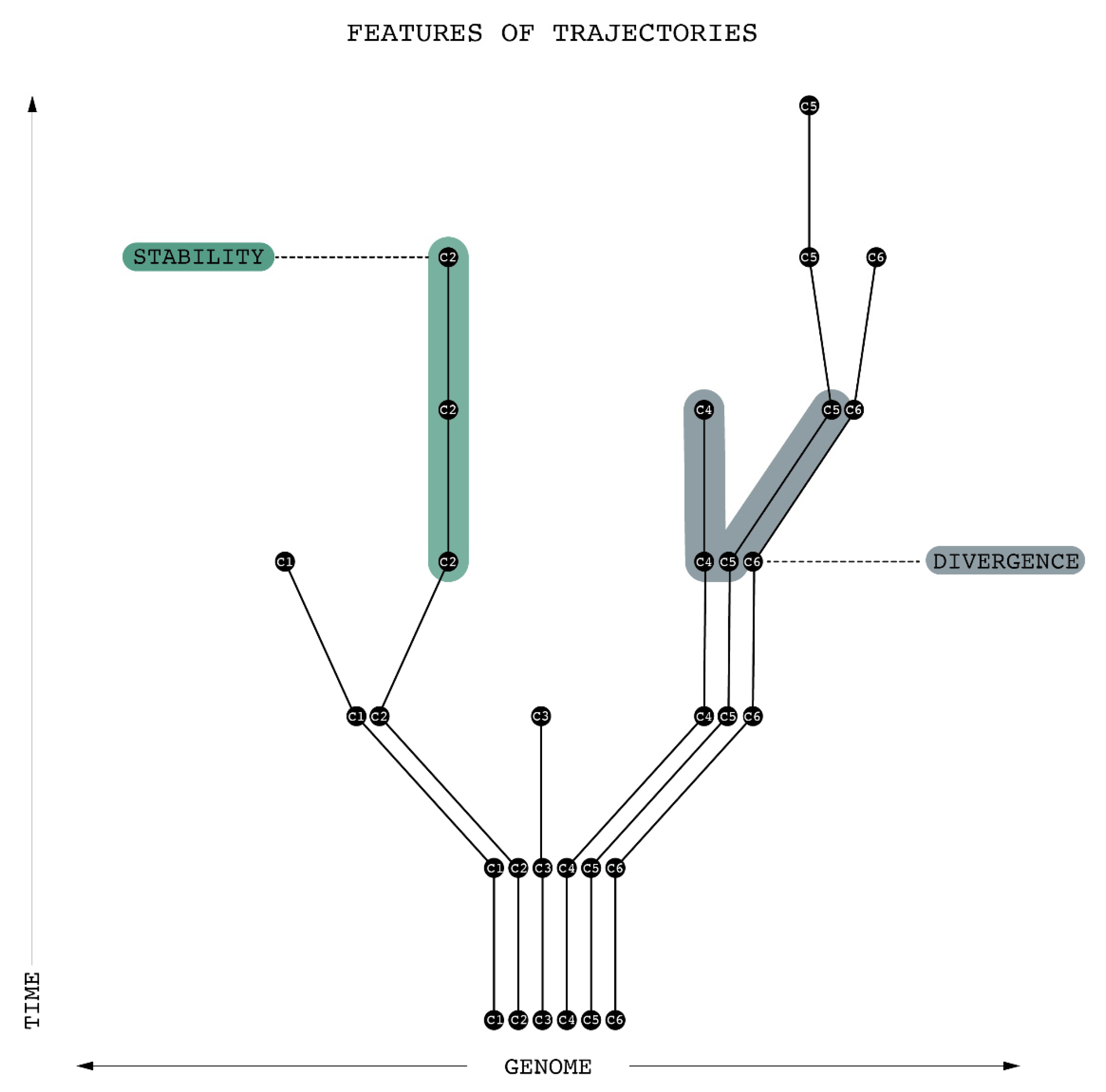
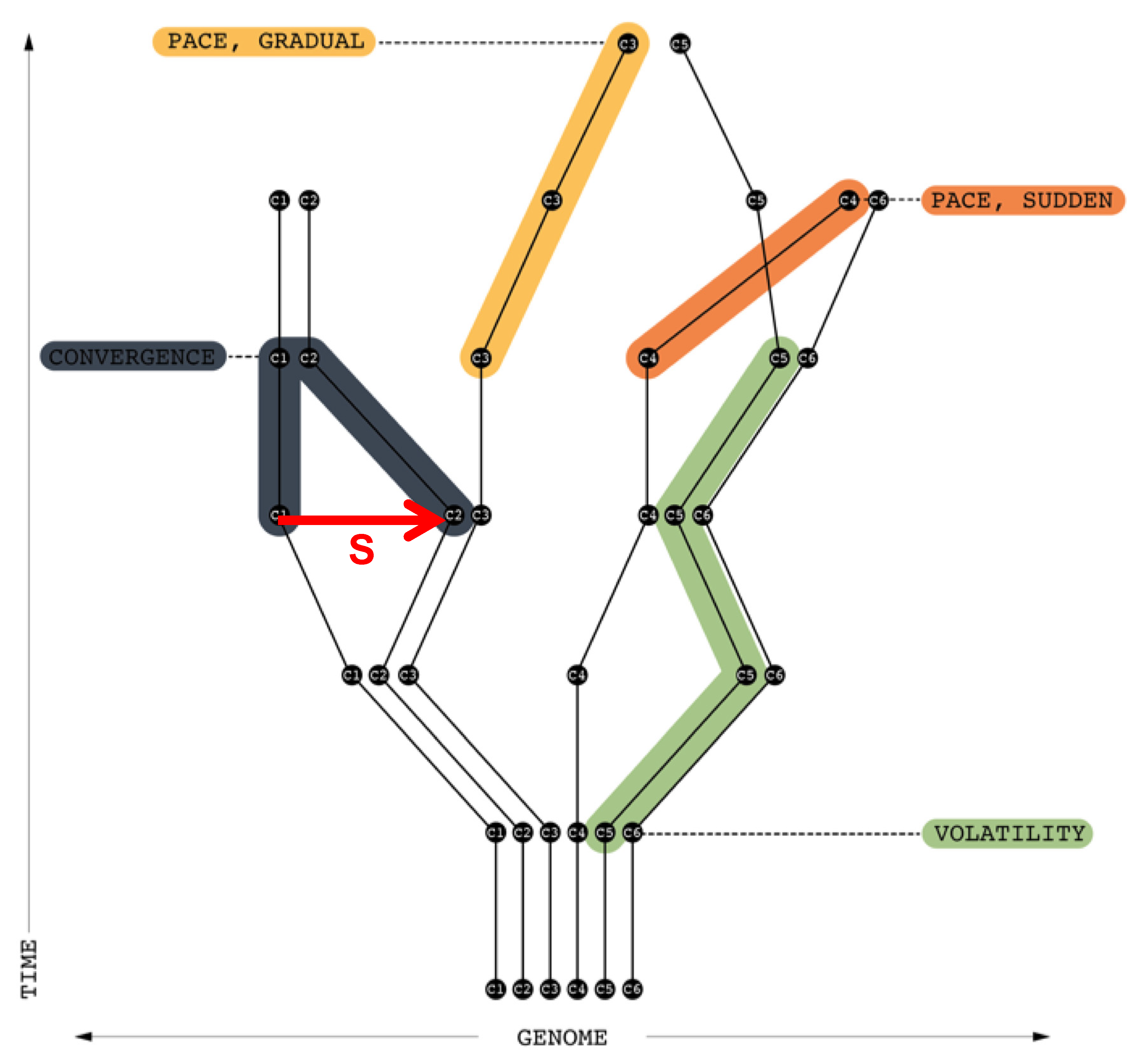
Using bFdist, we can visualize the evolutionary trajectories of the genomes of various spatial areas, i.e., bFdist(U₁, U₂). Figure 6 illustrates urban change in terms of the reproduction of urban genomes over time. Since moving up on the Y-axis represents the passage of time, the evolutionary lineage of different c can be traced by following a particular trajectory upwards. Along the X-axis, the diagrams provide a simplified depiction of genomic similarity between different c’s. Since proximity on the X-axis indicates a high degree of similarity, the diagram can be interpreted as representing the increasing differentiation of a set of spatial areas over time. Within this overall differentiation, characteristics such as pace, stability/volatility, and convergence/divergence (discussed in Part 3 [5]) govern the development of each individual c.

Figure 7 depicts the impact of signal s from c1 to c2. c2’s genome is modified so that its similarity to c1’s genome is increased, hence the bFdist() between c1 and c2 decreases over time—they converge. “Pace, Gradual” show how a c3’s genome gradually changes over time to be closer to c5 (i.e., reduction of formetic distance). “Pace, Sudden” depicts how c4’s genome undergoes a rapid change bringing it close to c6 in a short period of time. “Volatility” depicts how the genomes of c5 and c6 change each time step but stay foremetically similar during the first 4 time periods.

Consider two spatial areas that contain formemes for the same types of elements, i.e., groups, activities and physical forms, but differ in the frequency with which they appear. For example, a gentrified town in the country may contain formemes for the same types of elements as a neighbourhood in a big city, but differ in the overall size or frequency of the elements, i.e., more of each of the common forms, groups and activities. Are these two spatial areas the same? Or consider the same spatial area whose elements do not change over time but the size or frequency does. For example, an ethnic neighbourhood, such as Italian or Greek, attracts greater numbers of formemes for the same forms, activities and groups over time. Is this the same neighbourhood?

To account for these types of scenarios, we define an alternative Fdist which we refer to as the “weighted distance metric” wFdist. wFdist takes into account the frequency with which elements appear in a set of formemes. If two sets of formemes have the same elements, then bFdist will determine that they are the same, i.e., zero distance between them. However, if one set of formemes has a greater frequency of elements than the other, then the distance will be greater than zero.

$$\mathrm{wFdist}\left(\mathrm{F}1, \mathrm{F}2\right)=1-\frac{{{\displaystyle \sum }}_{\mathrm{e} \in \mathrm{Elements}\left(\mathrm{F}1, \mathrm{F}2\right)}\min \left(\mathrm{Fsize}\left(\mathrm{F}1,\mathrm{e}\right), \mathrm{Fsize}\left(\mathrm{F}2, \mathrm{e}\right)\right)}{{{\displaystyle \sum }}_{\mathrm{e} \in \mathrm{Elements}\left(\mathrm{F}1, \mathrm{F}2\right)}\max \left(\mathrm{Fsize}\left(\mathrm{F}1,\mathrm{e}\right), \mathrm{Fsize}\left(\mathrm{F}2, \mathrm{e}\right)\right)}$$

where Elements(F1, F2) is the set of all elements contained in F1 and F2,

Elements(F1, F2) = F1[p] ⋃ F2[p] ⋃ F1[g] ⋃ F2[g] ⋃ F1[a] ⋃ F2[a]

We define two additional distance metrics focused on Group and Activity.

gdist(g1, g2): measures the distance between two groups, g1 and g2. The lower the distance, the greater the similarity between the groups.

Axiom 1:	Reflexivity gdist(g, g) = 0
Axiom 2:	Symmetry gdist(g1, g2) = gdist(g2, g1)
Axiom 3:	Subadditivity gdist(g1, g2) + gdist(g2, g3) ≥ gdist(g1, g3)

adist(x,y): measures the distance between two types of activities, a1 and a2. The lower the distance, the greater the compatibility between the activities.

Axiom 1:	Reflexivity adist(a, a) = 0
Axiom 2:	Symmetry adist(a1, a2) = adist(a2, a1)
Axiom 3:	Subadditivity adist(a1, a2) + adist(a2, a3) ≥ adist(a1, a3)

5. Spatial Distance

Variation in a spatial area’s genome may be due to its closeness to other spatial areas; a type of “spill over” effect. To support variation propositions based on spatial distance, we introduce the concept of distance between spatial areas (

Table 1. Spatial Area Distance Metrics.

Relationship	Description
distanceC(ci, cj, t)	distance between the centroids of ci and cj
distanceB(ci, cj, t)	shortest distance between the borders of ci and cj

).

Axiom 1:	Reflexivity distanceC(c,c,t) = 0
Axiom 2:	Symmetry distanceC(c1, c2, t) = distance(c2, c1, t)
Axiom 3:	Subadditivity distanceC(c1, c2, t) + distance(c2, c3, t) ≥
	distance(c1, c3, t)

The same axioms hold for distance B.

6. Evolutionary Trajectories

In previous sections, the concept of evolutionary trajectory was introduced. In this section we formalize the concept of a trajectory.

The Gpath predicate captures the existence of a path between any two signatures:

GPath(c1, t, c2, t’) is true if there exists a path that links SIG(c1, t) to SIG(c2, t’) in the evolution tree

where

Axiom:	Reflexivity GPath(c,t,c,t) = True
Axiom:	Symmetry GPath(c1, t, c2, t’) = GPath(c2, t’, c1, t)
Axiom:	Transitivity If GPath(c1, t, c2, t’) ∧ GPath(c2, t’, c3, t’’) then
	GPath(c1, t, c3, t’’)

If we assume there exists a single phylogenetic urban lineage tree, that is a common lineage to which all urban forms can be connected, GPath would be unnecessary as any node (i.e., genome) in the tree can be reached from any other node, ignoring directionality. However, it is possible several trees co-exist, for example, as central American cities may have evolved separately to some degree from their European counterparts.

We define fPathU which determines whether two genomes that are connected (GPath) contain the same formeme f:

fPathU(c1, t, c2, t’, f) is true if GPath(c1, t, c2, t’) is true ∧ f ∈ UG(c1, t) ∧ f ∈ UG(c2, t’)

where:

Axiom:	Reflexivity fPathU(c, t, c, t, f) = True
Axiom:	Symmetry fPathU(c1, t, c2, t’, f) = fPathU(c2, t’, c1, t, f)
Axiom:	Transitivity If fPathU(c1, t, c2, t’, f) and fPathU(c2, t’, c3, t’’, f)
	Then, fPathU(c1, t, c3, t’’, f)

We define fPathH similarly but with f ∈ HG(c1, t) ∧ f ∈ HG(c2, t’).

In order to capture the concept of phylogenetic lineage and inheritance, we introduce a restricted version of path, a directed path, where a directed path exists between two signatures if there exists a GPath, and the first genome is an ancestor of the second. An ancestor of a signature s for spatial area c is another signature for c, or a spatial area that includes c, that occurs earlier in time.

DPath(c1, t, c2, t’) is true if GPath(c1, t, c2, t’) ∧ t < t’ ∧ c2⊆c1

where

Axiom:	Reflexivity DPath(c, t, c, t) = True
Axiom:	Asymmetry DPath(c1, t, c2, t’) ≠ DPath(c2, t’, c1, t) for c1 ≠ c2
Axiom:	Transitivity If DPath(c1, t, c2, t’) and DPath(c2, t’, c3, t’’)
	Then, DPath(c1, t, c3, t’’) for t < t’ < t’’

Normally, c1 = c2, i.e., we are following the changes in the signatures of a single spatial area over time. However, it is possible that c2 is contained in c1, meaning at some point the spatial area c1 was partitioned into sub spaces.

Similarily, we define fDpathU which determines whether two genomes that are connected (DPath) contain the same formeme f:

fDPathU(c1, t, c2, t’, f) is true if DpathU(c1, t, c2, t’) is true

∧ f ∈ UG(c1, t) ∧ f ∈ UG(c2, t’)

where

Axiom:	Reflexivity fDPathU(c, t, c, t, f) = True
Axiom:	Asymmetr fDPathU(c1, t, c2, t’, f) = fDPathU(c2, t’, c1, t, f) for c1 ≠ c2
Axiom:	Transitivity If fDPathU(c1, t, c2, t’, f) and fDPathU(c2, t’, c3, t’’, f) Then,
	fDPathU(c1, t, c3, t’’, f) for t < t’ < t’’

We define fDPathH similarly but with f ∈ HG(c1, t) ∧ f ∈ HG(c2, t’)

Finally, we introduce the concept of an environmentally stable trajectory. We define the environment of some spatial area c as stable between times t and t’, where t < t’, for some threshold k_s, if the Fdist of the two sets of Signals is less than k_s. In other words, the signals received during the time period are similar to each other.

Given: SIG(c, t) = <U, H, S, R> ∧ SIG(c, t’) = <U’, H’, S’, R’>

    Estable(c, t, t’) = True if Fdist(S[f], S’[f]) ≤ k_s, else False

7. Formeme Survival

Formemes may reproduce at different rates. Furthermore, as this occurs, the distribution of formemes in the total population of c’s will change. Some variants will cover a wider swathe of spaces, others will dwindle: the city evolves.

In evaluating formeme survival, reproductive strategies are crucial concepts, elaborated further in Part III [5]. We represent the set of selection strategies as 𝓡.

𝓡: Is the set of selection strategies that can be used to propagate a

     formeme or genome.

We represent the application of a replication strategy as:

UG(c,t’) = replicate(c, t, st)

where “replicate” applies replication strategy st to the genome UG(c,t) and st ∈ 𝓡.

To unpack the notion of differential reproduction, we need to develop a framework for discussing sets of formemes and urban hunomes: many areas (c’s) formed in different or similar ways.

We define a hunomeSet as a set of sets of formemes. Each set in hunomeSet is define by a hunome HG(c, t) where c is a member of a set of non-overlapping places C and t is a member of a set of times T.

hunomeSet(C, T) = { HG(c, t) | c ∈ C and t ∈ T }

The notion of hunomeSet allows us to examine formemes distributed across locations.

We define formemeCount(C, T, F) to be the number of members of hunomeSet(C, T) that contain the same set of formemes F.

formemeCount(C, T, F) = | {HG(c,t) | F ⊆ HG(c, t) ∧ c ∈ C ∧ t ∈ T}|

Formemes will exhibit variation over both time and space. The question is which will survive? For any hunomeSet, the survival rate of a subset of formemes is given by the total members for a hunomeSet at a given time that contain F, divided by the number of members at a previous time:

formemeSurvivalRate(C, F, t, t’) = formemeCount(C, t’, F) / formemeCount(C, t, F)

where t’ > t.

If formemeSurvivalRate is less then 1, then the occurrence of the formeme set F is decreasing over time, and as the survival rate approaches 0, a set of formemes approach extinction.

Finally, we can extend the notion of survivalRate to activities as follows:

activitySurvivalRate(c, a, t, t’) = size(c, t’, a)/size(c, t, a)

8. Activity Costs and Recoding

Our model of urban evolution provides a vocabulary for representing how and why various traits of the urban environment replicate at different rates in different places. To formulate such a model, we need to cover some additional ground: activity costs and recoding. These terms give us language to explain how and when U changes (or persists), and to characterize the difference between genomes that are geared toward restrictive and highly specific uses/users (those that impose clearly defined costs on specific uses and users) vs. those that are more flexible and less clearly controlled. The notion of “control” allows us to conceptualize how the reproduction of formemes can be governed by institutions and depends on the power relations between source and receiving areas. We elaborate the implications of this idea in Part III’s discussion of “power bias” in evolutionary selection.

We define the cost of performing some type of activity a in reference to a set of formemes F by the following function:

activityCost(F, a) where F is a set of formemes.

Cost is indicative of resistance. If we are speaking of a dance club, this means that it requires relatively little cost to use it as such. Conversely, violating its code can come at great cost. Somebody who tries to drive a semi-truck onto a narrow road meets resistance from the physical form; somebody who attempts to walk into a nightclub in violation of the dress code meets resistance from the bouncer; and somebody who attempts to undertake activities in violation of a zoning designation meets resistance from city inspectors. These are examples of activities for which their costs depend on the genome.

Proposition:

if e ∈ F[a] and e’ ∉ F[a], then activityCost(F, e’) > activityCost(F, e).

In other words, it will generally be more difficult to perform an activity in a formeme set for something it is not currently programmed.

We define aggregateActivityCost as the sum of activityCost of all activities a in formeme set F:

aggregateActivityCost (F) = ∑ _e∈F[a] activityCost(F, e)

It can be the case that it is more difficult for one group to participate in an activity than other. One example is the direct or indirect segregation of activities. Assume that there is a single golf course in c, and membership/usage is controlled by a membership committee who limit membership to their own group. Attempts by members of other groups to join or use the golf course are rejected by the committee. Once in a while an outsider may be admitted if they have high enough prestige or donate substantial sums of money. We capture the concept of differential cost of activities by groups in the context of a set of formemes F as:

groupActivityCost(F, a, g) where a is the activity performed by group g

      in c, at time t.

The genome for a space c can remain stable over time, or it can change. When genomes change, they have been recoded. Recoding an area’s genome means that variant formemes have been retained there. For example, a location with a warehouse programmed for shipping and receiving that changes to a dance club has been recoded. Recoding involves adding, removing or modifying formemes. We can identify a specific occurrence of recoding as follows:

Recoding: UG(c, t1) ≠ UG(c, t2) for t2 > t1

Here, the fact that UG(c, t2) differs from UG(c, t1) indicates that location c at some later time t2 has been recoded in some fashion.

Recoding is not always easy, because encoding a space c imposes a cost structure favouring or hindering some uses and users. The physical form of a warehouse, for example, is relatively conducive to dancing to loud music, but also to shipping and receiving. It offers substantial open space and sound dampening. Likewise, a building code imposes costs on changing the physical materials and arrangement of a form. Similarly, a dress code imposes relatively high costs on users who attempt to violate it.

Because variation in recoding costs affects the transmissibility of formemes, it also generates the path dependencies out of which evolutionary historical trajectories arise. Recoding costs in this way capture the underlying mechanisms that produce urban analogs of genotypes in contrast to phenotypes. While all observable traits in an area may be considered parts of its phenotype, only those that permit recoding may transmit formemes. For example, in an area with an extremely strict building code, changes to a building during its life course that are inconsistent with the building code will not affect future buildings in the area, unless those changes become embedded in the building code. By contrast, if there is no building code and recoding costs are very low, almost any observable feature in an area can spread formemes that influence other buildings.

We represent the cost of recoding a set of formemes F into a set F’ as:

R(F, F’)

In other words the cost of changing the form, activity and/or users in any of the formemes. R(F, F’) could be viewed as the sum of the independent recodings of the formemes in F. Note that R(F, F) = 0.

Finally, the definition of the recoding cost function R is specific to a signature. If a signal’s formeme s[f] is used to recode the genome U, then a new recoding cost function R’ is derived by applying the signal’s recoding cost transform to the original recoding cost R:

R’ = s[r](R).

9. Discussion and Conclusions

Our model of urban evolution is driven by the distinction between: the Urban Genome U, which defines the information encoded in a spatial area regarding how to organize the space physically, and for certain groups and activities; the information informing human actors H who frequent the space; and Signals S, the formemes transmitted in the spatial area. This distinction allows us to formulate evolutionary rules (see part III [5]), for example about how the frequency of signals, such as the global rise of coffee culture, can impact H; or how changes in H, such as new attitudes about the uses of buildings, can impact U.

Central to this model is the Formeme. A Formeme encapsulates the binding force between form, groups, and activities. It is the foundational component that underlies U, H and S. It is Formemes that are communicated by Signals. It is Formemes that define both U and H.

The model raises a number of questions, which we address by way of conclusion.

• What is the appropriate size of a spatial area c?

By design we do not constrain the size of a spatial area. A spatial area can be as small (or large) as a building, a city block, a neighbourhood, a census track, or the entire city. The spatial areas chosen depends on the focus of the analysis. For example, we may want to study the evolution of the groups and activities of a single neighbourhood independent of others. Or we may want to study the impact of signals on several contiguous neighbourhoods, each represented by a separate c, but each sending signals to each other. Or we may want to study the neighbourhoods separately and in aggregate, where the neighbourhood spatial areas are contained within the city spatial area.

• What are the possible elements of the components: P, G and A?

The answer depends on what is being studied. For example, if we are studying the evolution of Pueblo Societies between A.D. 600 and 1300 [11], the elements of P, G, and A would be very different than if we were studying a rural village today. The choice of elements depends upon what is being studied and the hypotheses driving the study; the elements chosen to model the same spatial area for the same time period may differ from one researcher to another, reflecting their own research hypotheses. The elements chosen to model a set of spatial areas at one level may also differ from the elements used to model an aggregation of these spatial areas, i.e., neighbourhood level elements versus city level elements. Perhaps part of the evolutionary process is selecting and/or aggregating elements to be used at an aggregate spatial level.

• Does the model scale?

It depends on what is meant by scale. Certainly, spatial areas can be as small as needed, such as a city block, and as large as a city. Furthermore, they can be analysed simultaneously, as the model supports as many levels of spatial aggregations as needed, and alternative aggregations. Moreover, elements can differ between levels of abstraction, allowing for aggregation and abstraction of elements, thereby making for a powerful approach to modelling and analysing scaling.

• How does this relate to agent-based urban simulations?

One can view an agent-based simulation as generating the data necessary to construct the Urban Signature. An event in an agent based simulation generates a quintuple comprised of a time, a spatial area, a group (which can be an individual), an activity (the event) and a form (where or on what the activity has been performed) (We have omitted discussion of Signals for simplicity). These event generated quintuples can then be used to generate the hunome H. In other words, based on these events we can construct a spatial area’s signature for different periods of time. We can then study how H changes over time, and how it in turn changes the genome U.

• A Signature can represent the form, activities and groups at some space and time, but where does evolution appear?

With the Signature defined, we can now explore the evolution of urban areas by generating and analysing the changes in an area’s signature over time through the basic evolutionary algorithm of variation-selection-retention, as elaborated in Part III [5]. Assuming a source of event data, either from a simulation as discussed above, or from datasets such as Yelp, Foursquare, Google, national censuses, etc., for each combination of spatial and time period we can generate a Signature. We can then analyse a spatial area’s signature over time to see how H and S interact and lead to changes in U. In other words, the Signature provides snapshots of what we believe are the key components of an urban area, which we can use either to infer rules of urban evolution, or confirm/refute hypothesized rules of urban evolution.

• What about intangible elements that take part in the construction of urban spaces?

Regarding the incorporation of “intangible elements which take part in the construction of urban spaces, e.g., socio-cultural ideologies, values, perceptions etc,” as well as human agency, the model does not explicitly focus on HOW ideologies, values, etc. affect the choices made by groups in the evolution of a space. The model does allow for the differentiation of groups, activities and forms, enabling the representation of groups with differing ideologies, etc. and their corresponding forms and activities. Part III [5] develops this idea in a somewhat minimal way through the idea of “content dependence” we articulate there, but certainly there is room for more elaborate propositions about the how formemes become more or less attractive to different groups. Clearly, the urban environment is complex, and models of choice, including constraint networks, are needed to model and understand in detail why choices are made. Never the less, the model is intended to provide an abstraction of a space that simplifies evolutionary analysis so that significant traits can be identified and their evolution traced.

Part I [1] of our Model of Urban Evolution situated our work with the broader context of the study of cities and theories of urban and cultural evolution. Part II has formally defined our model of a city, and in fact any urban, suburban or rural area. These two parts prepare the way for Part III where we introduce our rules of urban evolution.

Part III [5] develops a formal model of urban evolution in terms of (1) sources of variations; (2) principles of selection; and (3) mechanisms of retention. More specifically, regarding (1) it defines local and environmental sources of variation and identifies some of their generative processes, such as recombination, migration, mutation, extinction, and transcription errors. Regarding (2), it outlines a series of selection processes as part of an evolutionary ecology of urban forms, including density dependence, scope dependence, distance dependence, content dependence, and frequency dependence. Regarding (3), it characterizes retention as a combination of absorption and restriction of novel variants, defines mechanisms by which these can occur, including longevity, fidelity, and fecundity, and specifies how these processes issue in trajectories define by properties such as stability, pace, convergence, and divergence.

Part IV [6] applies the models developed in Parts II and III to the evolution of neighbourhoods in Toronto and Montreal. Using Yelp data as a proxy for forms, groups and activities, neighbourhood signatures are defined. Using these signatures, the evolution of neighbourhoods are analysed and formetic distances are determined both longitudinally and transversally between Toronto and Montreal.