Geographically Weighted Regression-Based Predictions of Water–Soil–Energy Nexus Solutions in Île-de-France

Abstract

Due to global urbanization, urban areas are encountering many environmental, social, and economic challenges. Different solutions have been proposed and implemented, such as nature-based solutions and green and blue infrastructure. Taking into consideration exogenous factors that are associated with these solutions is a crucial question to assess their possible effects. This study examines the possible explanatory factors and their evolution until the year 2054 of several solutions in the Île-de-France region: wastewater heat-recovery, surface geothermal energy, and heat-mitigation capacities of zones. This investigation is performed by a series of statistical models, namely the ordinary least squares (OLS) and the geographically weighted regressions (GWR), integrated within a geographic information system. The main driving factors were identified as land use/land cover and population distribution. The results show that GWR models capture a large part of spatial autocorrelation. Apropos of prediction results, areas with low, medium, and high potential for implementing specific solutions are determined. Furthermore, the implementation capacities of solutions are compared with the demand depicted as the need for slowing down the effects of surface urban heat islands and the dependence on fossil energy. Moreover, the heat mitigation capacities are not at all times distinctively linked to human activities. Further investigations are needed to discover the remaining possible reasons, particularly air quality, water, vegetation, and climate change.

1. Introduction

Due to rapid urbanization, European cities are encountering a lot of environmental, social, and economic challenges [1]. The European Commission [2] summarized these challenges as risk and disaster management, poverty and social equity, degradation of natural and green areas, degradation of water and air quality, impacts of urbanization on human health, climate change adaptation, provision of ecosystem services, cost-effective infrastructure (as the initial capital expenses and the cost of on-going operations represent about 3.8% of the global gross domestic product in the year 2013), and the sustainable development.

Nature-based solutions (NBS), as well as green and blue infrastructure (GBI), emerge as cost-effective solutions and answers for these challenges [3] and will result in multiple benefits at the environmental and socioeconomic level, as well as for society and for public health [2,4]. These solutions, seeking sustainable development, could be implemented by harnessing the beneficial hidden sides of nature and infrastructure to turn socioeconomic and environmental challenges into innovative benefits and convenience. Despite the low number of research papers discussing the participation of stakeholders in NBS in Europe up to the year 2020 (e.g., 76 publications in all European countries; 5 in France), the European Union Research and Innovation (R&I) agenda on nature-based solutions pointed out that “Europe will become a world leader both in R&I and in the growing market for nature-based solutions” [1,2]. To this end, understanding the effectiveness of these solutions is necessary before implementation; this requires a systemic approach that incorporates the technical measures’ regulatory, governing, financial, business, social, and geographical sides. In gross, the benefits can be depicted particularly in terms of: (a) exhaustive energy consumption (EC) and the questions of renewable sources of energy, (b) mitigation of heat and environmental risks, and (c) the economic burden of operating, protecting, and maintaining the traditional non-natural infrastructure, particularly for water drainage and management. More precisely, these solutions, considered to be urban innovations, stem from interactions between different domains such as: (i) soil–energy interactions, for instance, the geothermic production [5,6,7]; (ii) wastewater–energy interactions, such as the fatal HR [5,8,9]; (iii) green spaces–air temperature interactions: urban cooling, and enhancing air quality [10,11]; (iv) soil–water interactions: water management, flood mitigation, and water recharge [12]; (v) soil–vegetation interactions: carbon storage [10,11], etc.

However, according to the scientific literature review, no systemic study has investigated all the possible interactions in the urban context, but only limited disciplinary approaches. Examples of these studies are those of NBS and GBI that focus on urban cooling and water management—the studies of local energy production (as fatal heat recovery (HR), geothermic production, and solar energy), and those examining the solutions to enhance air quality. Furthermore, almost all these solutions require space to be implemented, and this could lead to possible competition for space between these solutions. In addition, the existing territories are highly constrained by their histories, topographic specificities, and urban configurations: suggesting marginal evolution rather than a design from scratch. This spatial competition is also not well recognized or analyzed. 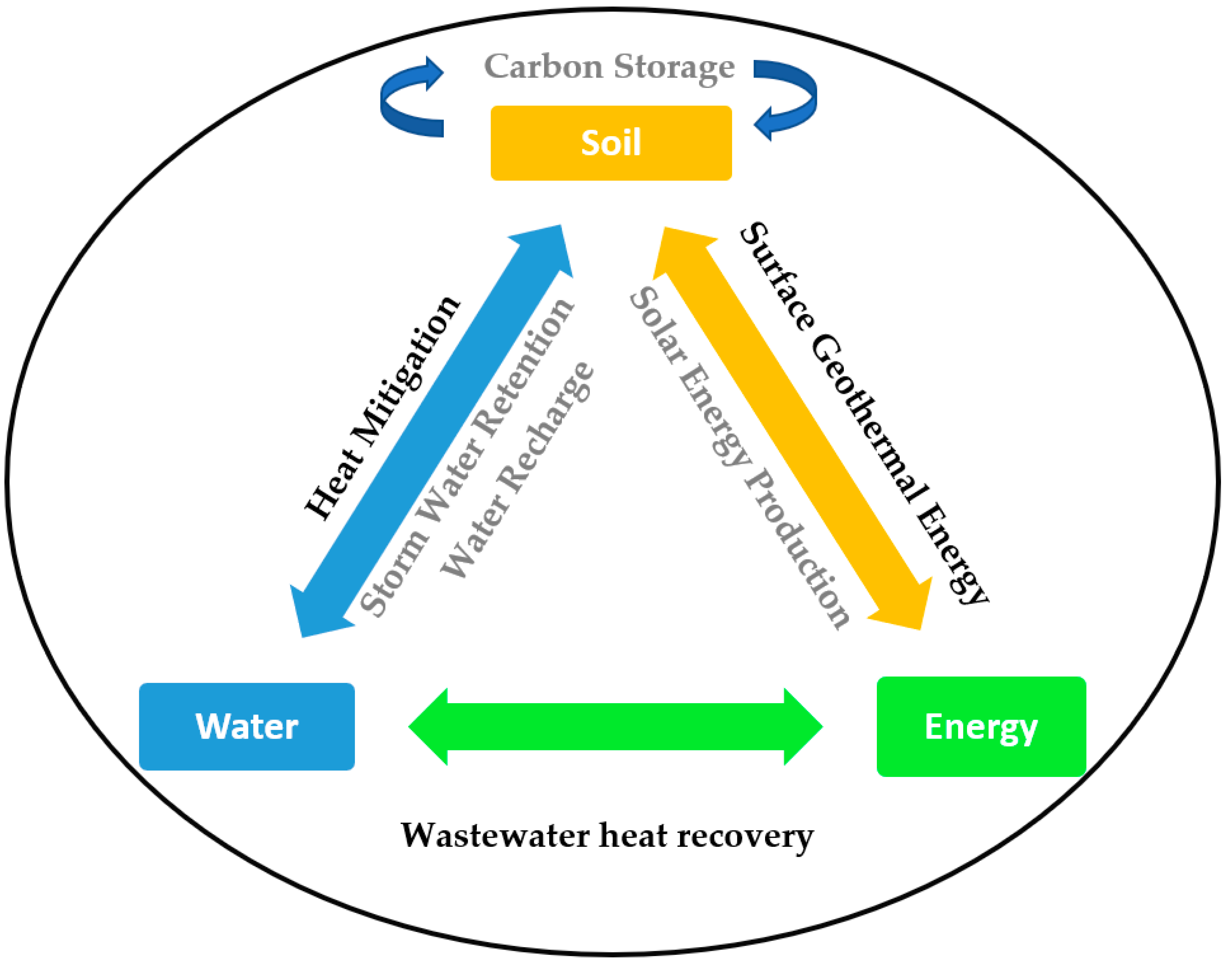The aforementioned spatial analysis is essential for decision support, especially when comparing the alternative solution in an integrated policy–science–society framework [1]. This paper identifies the elements of three interacting spheres that are relevant to study urban innovations: (a) soil: the historical actor in urban development, space allocation, vegetation, imperviousness, albedo; (b) water: a crucial element necessary for life, but also a possible threat (storms, floods, etc.), stock and flow processes; and (c) energy: a crucial element, hard to produce in an urban setting, hard to store (batteries) and to transport over large distances. It is noteworthy to mention that both water and energy must be saved in the context of sustainable development. In the context of this research, all the solutions that cross at least two dimensions of the water–soil–energy nexus (WSE nexus) are envisioned. Attention must be drawn to the fact that NBS and GBI are part of the WSE nexus. Figure 1 shows the most commonly known WSE interactions.

According to the literature review presented in the following subsection and to the best of the authors’ knowledge, the links between existing WSE solutions and urban characteristics, as well as the potential for further implementation of WSE solutions, are still unclear. As a result, these relationships are not well recognized and understood by institutional, political, and ruling authorities and official decision-makers, especially when they enact energy/environment-based policies. As a consequence, this could generate suboptimal sustainable development decisions.

Therefore, this paper aims to analyze the links between existing WSE solutions and urban characteristics in conjunction with the assessment of the potential for further implementation of WSE solutions in the Île-de-France area. This analysis aims to provide a clear picture of WSE solutions–urban interactions for the governing bodies and local authorities. Several hypotheses are proposed for validation. Among these suppositions, it is hypothesized that the dense urban areas (with high population density) represent good candidates for the implementation of wastewater HR solutions. In the same direction, medium to low urban areas are suggested to represent good candidates for the implementation of surface geothermic solutions. The hypotheses are also extended to assume that the implementation of some WSE solutions (notably HR) is attributed, in general, to political decisions rather than to factors from the urban context. Regarding limitations, this paper analyzes only the WSE nexus in the urban context and the potential of implementing these solutions from a spatial context, particularly the renewable energy sources and the WSE solutions to reduce the land surface temperature.

The solutions are designed to mitigate the risk of climate change, floods, and air pollution and to ensure that biodiversity protection is not investigated for further predictions. In particular, the impact of green roofs and vegetated facades on the quality and temperature of the air, as well as the effects of solar energy on fossil energy consumption, are not investigated due to limited available data and information about the explanatory variables. Several previous studies have investigated the different naturally and artificially established interactions between soil, water, energy, and vegetation. An overview of recent relevant studies is presented as follows. Various studies examined the effectiveness of operating different NBS (vegetation in particular) for better water management, ecosystem integrity, and biodiversity protection. For instance, Pander et al., Schindler et al., and Funk et al. [13,14,15] examined the effects of reconnecting rivers to floodplains, by removing barriers along the river course in the Danube floodplain in Germany and in different countries of Europe on reducing the soil erosion, flood mitigation, and water purification. Similarly, the effects of green infrastructure, such as (i) reforestation, (ii) green roofs, (iii) maintaining vegetation cover and good soil structure, and (iv) the construction of shallow water bodies with vegetation, such as wetlands, on water management have been analyzed in the studies of Perni and Martínez-Paz in Spain [16], Majidi et al. in Bangkok, Thailand [17]; Soana et al. in Italy [18], and Harrington et al. in Ireland [19], respectively. Furthermore, the importance of green corridors and their associated drainage capacities in protecting the rail infrastructure, particularly in the case of extreme weather events, were examined by Blackwood et al. [12]. In addition, the green infrastructures/infrastructure network, such as the green corridors, ensure the security of regional ecology by maintaining the ecosystem’s integrity and conserving biodiversity [20,21]. Other studies examined the cost efficacy of NBS, in the manner of afforestation, in supporting biodiversity and protecting the ecosystem services, such as in the study by Seddon et al. [22], and in the vein of using high-albedo-pervious pavement material to slow down global warming and to mitigate heat and climate change as in the study of Majidi et al. [17]. Similarly, Blackwood et al. [12] explained how green corridors could support climate change adaptation and protect the transport infrastructure (e.g., rail services), specifically during extreme weather events.

Recent analyses were carried out to examine how to increase the sustainability of the use of matter and renewable energy [23]. For instance, the HR from hot commercial, industrial, and domestic wastewater to reuse for residential heating demands, using technologies such as heat pumps and heat exchangers, was examined in different studies [24,25,26]. Dürrenmatt and Wanner [27] indicated that the process of HR is explained by two phases, (1) the thermal conductivity between the wastewater and the pipe wall, which temporarily store the heat, and (2) the recovery of energy by heat transfer from the wall of the pipe with the help of a heat exchanger and a heat pump. The wastewater HR process could be implemented at different scales as the wastewater treatment plants [9,28], the sewer network level, and the building level [24]. The authors pointed out that the HR process could supply heat energy to individual buildings as well as to large communities. With a further detailed inspection, the wastewater treatment plants have a high potential to provide heat energy and feed urban areas, however, the efficiency of the system integration depends on the timeline grid of energy supply and demand as well as the spatial contiguity between the treatment plant and the beneficiaries [9,29]. On the other hand, surface geothermal energy (SGE) also represents a new way to reduce the consumption of fossil energy, particularly for home heating and cooling [6,7]. The SGE is used for air conditioning, such as cooling applications, as well as heating needs [7]. The authors explained the setting up of the system as the deployment of a ground source heat pump system composed of a horizontal ground heat exchanger connected to a reversible geothermal heat pump that is connected to a chilled ceiling panel system.

In order to analyze the links between existing WSE solutions and urban characteristics of the surrounding areas as well as to predict the potential for future implementation of WSE solutions, the following summarized sequence is respected: (1) choosing a terrain: part of the Île-de-France region; (2) examining some implemented WSE solutions (e.g., HR from hot wastewater, SGE, forest development…); (3) characterizing the intensity (e.g., HR) or the effectiveness (e.g., heat mitigation (HM)) of the WSE solutions; (4) setting-up a statistical model (geographically weighted regression GWR) between the WSE characteristics and the urban characteristic (e.g., population, infrastructures…); (5) assessing the potential for further implementation of WSE solutions with the help of predictions for urban characteristics in the horizon of the year 2054; and (6) analyzing the possibilities for implementing the WSE solutions against the spatial demand represented by the need for this solutions. The year 2054 was selected (a) since it represents, from the current year, a sufficient time horizon to implement and evaluate the strategies proposed in this research, and (b) since the land use is projected for this year using the Cellular Automata Markov Chain Model (CAMCM) based on available data. With regards to GWR, these models are frequently used to link air temperature [30] and the variation of the surface urban heat island [31] to their influencing factors, such as the distance from water bodies and the vegetation cover. Nonetheless, and to the best of the author’s knowledge, there is no research study that employs the GWR in holistically examining the WSE nexus with its driving factors.

For the brief, this paper aims to (1) analyze the extensive (i.e., forestry development) and intensive (e.g., HR of wastewaters) components of WSE solutions, and (2) identify bottlenecks (e.g., saturation of urbanization in the north: forests are very unlikely to be developed there) and perspectives for the Greater Paris region. The paper is organized as follows. After the introduction, the second Section addresses the selection of the study area, the used research methodology and the data collection methods. The third Section presents the structure and the characteristics of the used models. The fourth Section summarizes and discusses the results and the fifth Section summarizes the main concluding remarks of the study and its limitations, and proposes new topics for future research.

2. Materials and Methods

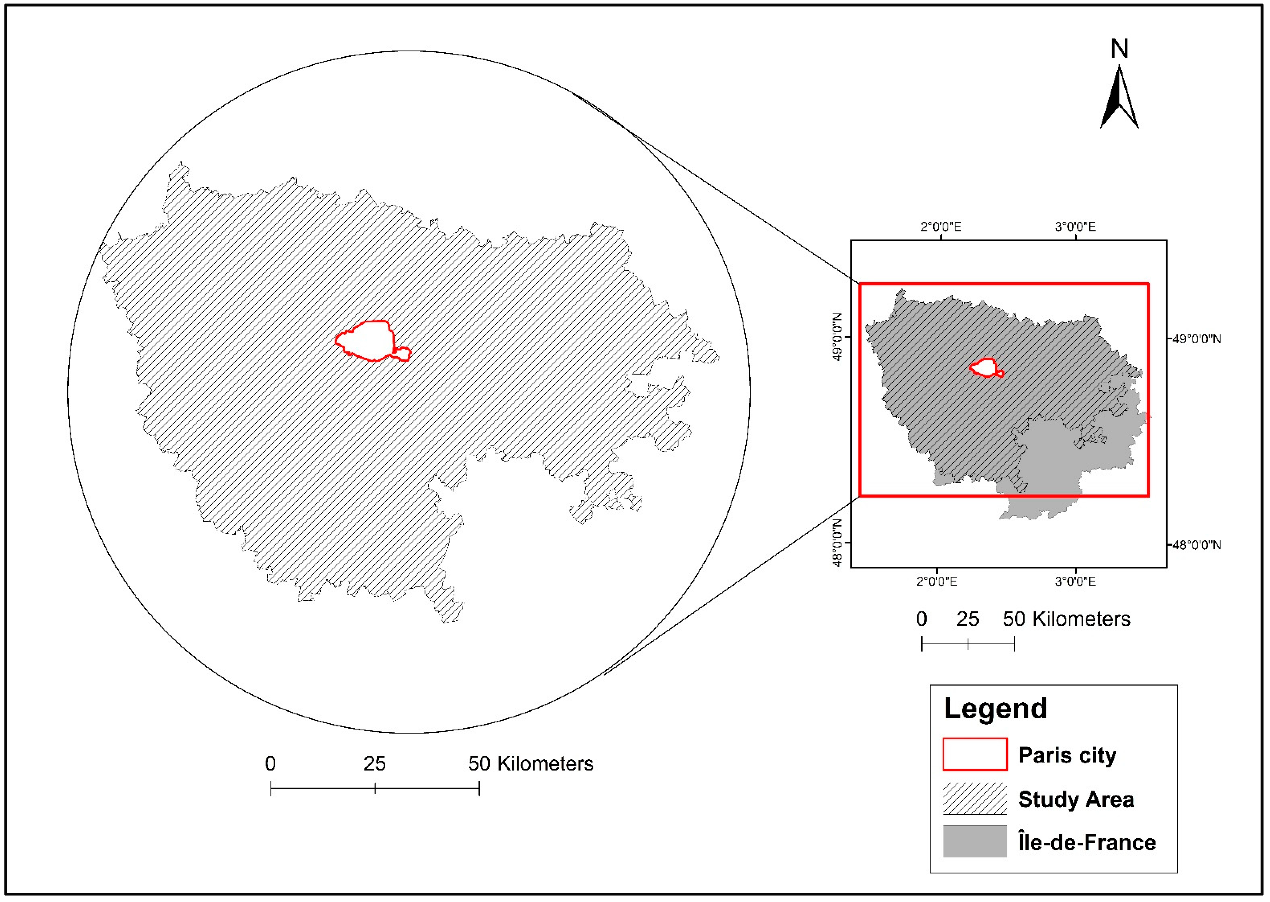
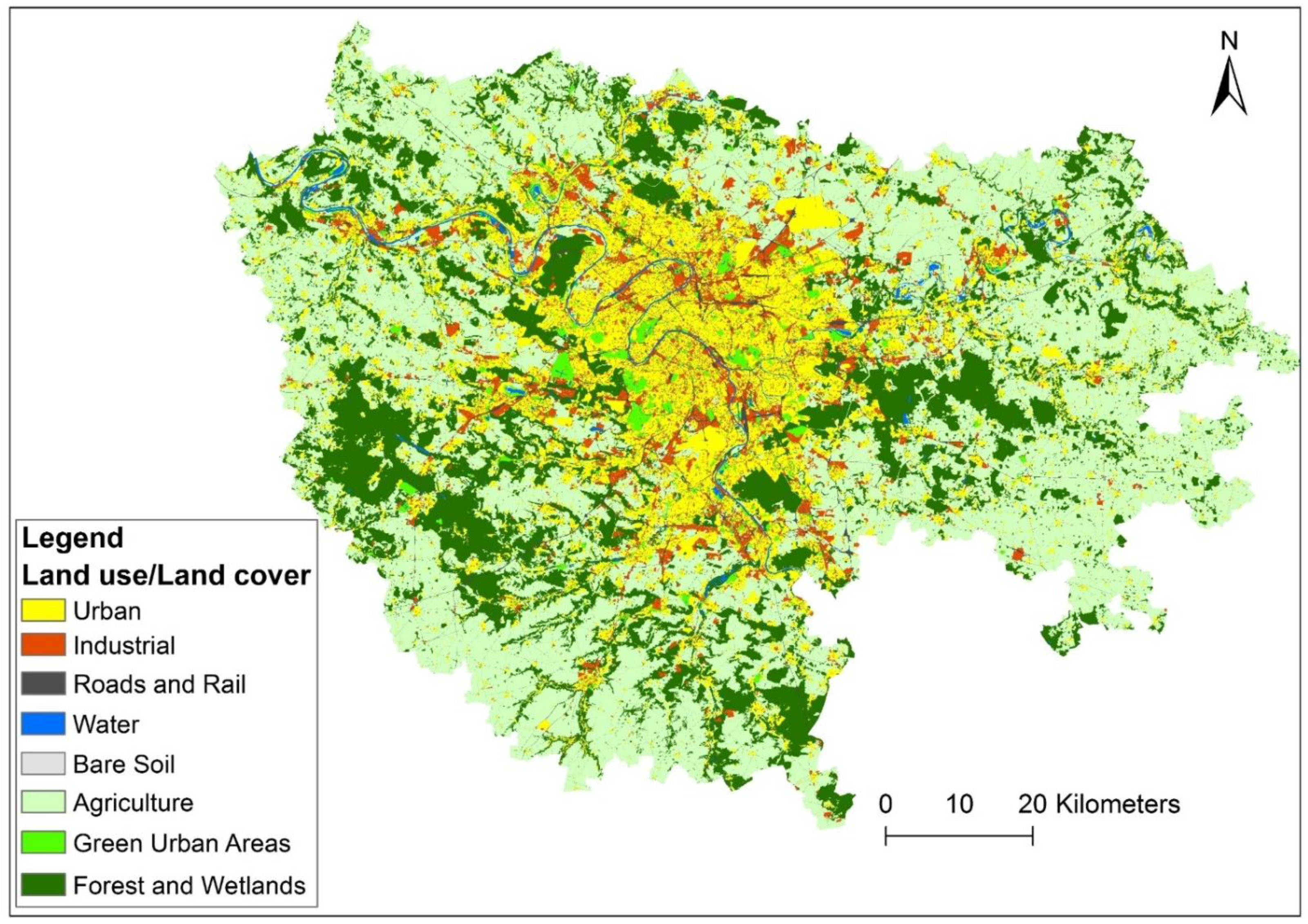
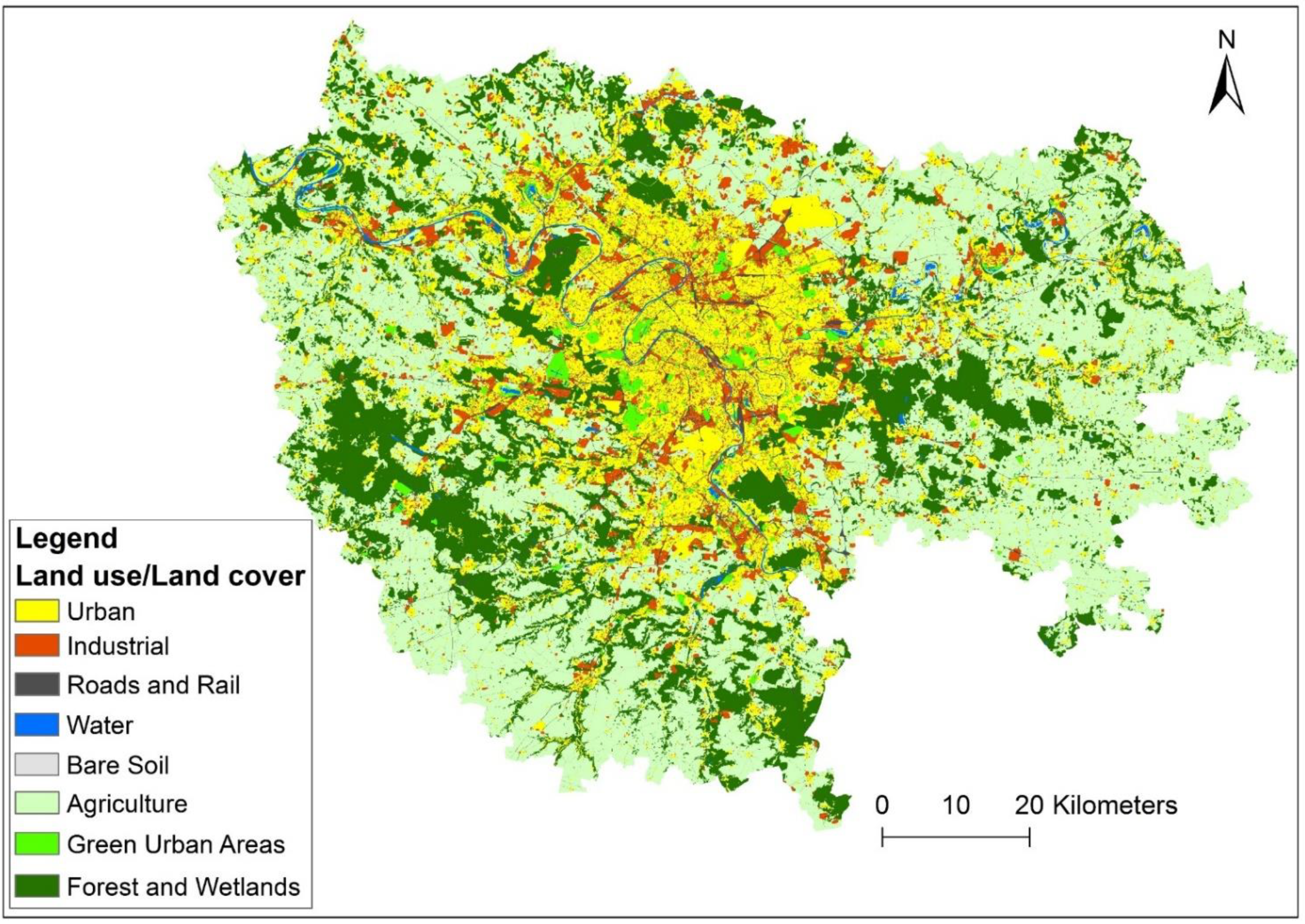
Examining the possible benefits of implementing solutions from the WSE nexus, as the relationships that could be established between energy production and consumption, usage and management of water and soils, is the main focus of this study, which was undertaken as part of a larger research effort, the “Wise Cities” project. This project examines the potential benefits of implementing solutions in this area both from the technical and managerial sides. It focuses mainly on the relationships between water and soil and between water and energy. This Section consists of two parts: the first one refers to the selection of the study area, and the second part presents the adopted research methodology, the needed data, and the data collection technique. The study area, which covers the most developed urban zone of the Île-de-France region, extends over 9261 square kilometers. As the envisioned work presented in this paper is the assessment of several water–soil–energy solutions, such as the fatal HR and the recovery of SGE, the area of interest, which covers a large area of the Île-de-France region, was selected because different types of these solutions have been implemented there in several places [5,32,33], and the required data are mostly available. The southeastern part of the Île-de-France region, which is outside the main agglomeration of Paris and for which the data are not available, is not included in the area of interest. Nonetheless, the study area is large enough to have proper data in order to be adopted to conduct the analysis. Regarding the analysis, the study area was selected to identify the key drivers of WSE solutions and to assess the possibility to predict their evolution. The predictions are envisioned for the horizon of the year 2054. Figure 2 shows the area of interest.

The methodology consists of predicting and analyzing the potential changes in some essential elements of the water–soil–energy nexus, such as the SGE, as well as recovering heat energy from wastewater and afforestation/reforestation to assess the possibility of implementing these concepts, especially in high-demand areas. Applying these measures intends, in general, to reach sustainable development as the main objective. In a more detailed way, the objectives within the WSE nexus are depicted by (i) reducing the need for fossil energy by developing natural and recycled sources of energy, such as the SGE and the HR from hot wastewater, (ii) enhancing the use of renewable sources of energy, and (iii) reducing the land surface temperature and limit the emergence of the surface urban heat island phenomenon. In this perspective, the main factors to be examined are (i) EC, (ii) SGE, (iii) HR from wastewater, and (iv) the capacity for HM. To this end, the identification of explanatory variables, as well as the use of statistical and regression models as the correlation analysis, ordinary least squares (OLS), geographically weighted regressions (GWR), spatial autocorrelation, and variance analyses (ANOVA), could give an overview of the significant explanatory variables of dependent variables, their effect sizes, the possibility to calculate spatial regressions, and the possibility to predict the future changes/evolutions of these variables. At greater length, the identification of explanatory variables is conducted through logical reasoning of the common driving factors. The correlation analysis, which is the part that comes next and represents the first data filter, is used to refine the data by keeping only the representative variable and removing the remaining factors among the observed collinear variables.

The following step is the selection of the variables by conducting the second data refinement process presented by the ordinary least square regression model (OLS).

A particular variable can be modeled (or predicted) using the OLS, one of the general linear modeling techniques, if this variable can be explained (as a regressive dependence relationship) by other explanatory variables [34] as indicated in the following equation:

$$y_i={\beta }_0+{\displaystyle \sum }_{j=1}^n{\beta }_j{X}_{ij }+{\epsilon }_i$$

(1)

where β₀, intercept; β_j, regression coefficients; X_ij, explanatory variables; ε_i, random errors with mean 0 (uncorrelated with one another).

Different trials are conducted to check the best-performing OLS model by checking the adjusted coefficient of determination (R2), as well as the multi-collinearity of variables and the overall multi-collinearity of the model, in addition to the spatial distribution of the standard residuals and their z-scores. The spatial autocorrelation is used to measure the correlation among residuals caused by their spatial location [35]. Usually, this test is used to check the existence of interactions between the residuals that are induced on the grounds of the spatial location of the observations. The spatial autocorrelation is a necessary measure to know whether the autocorrelation is significant or not. This latter concept could give information where the value of a residual is dependent or not on the values of neighboring residuals, so then the scale of the spatial dependence is determined by the geographic range within it the autocorrelation is significant. The following step is the application of the geographically weighted regression (GWR) in order to determine the regression relationship between the dependent variables and their explanatory variables, and also to establish a basis for the prediction process of future changes. The GWR is similar to the OLS model, however, the difference is depicted by taking the values of variables for each of the spatial features individually according to their spatial distribution. The GWR was developed as a solution for the problem indicating that the regression model estimated over an entire study area could not sufficiently cover local variations [35]. A particular variable can be modeled (or predicted) at different spatial spots using the GWR model based in a dependence-regressive way on several explanatory variables following Equation (2).

$$y_i={\beta }_{0\left(u_i,v_i\right)}+{\displaystyle \sum }_{j=1}^n{\beta }_{j\left(u_i, v_i\right) }{X}_{ij}+{\epsilon }_i$$

(2)

where u_i and v_i, spatial coordinates of observation I; β₀, intercept at point (u_i, v_i); β_j, regression coefficients at point (u_i, v_i); X_ij, the explanatory variables at point (u_i, v_i); ε_i, random error with mean 0.

The sequence of these processes, used to predict the changes in the dependent variables, is presented in Figure 3.

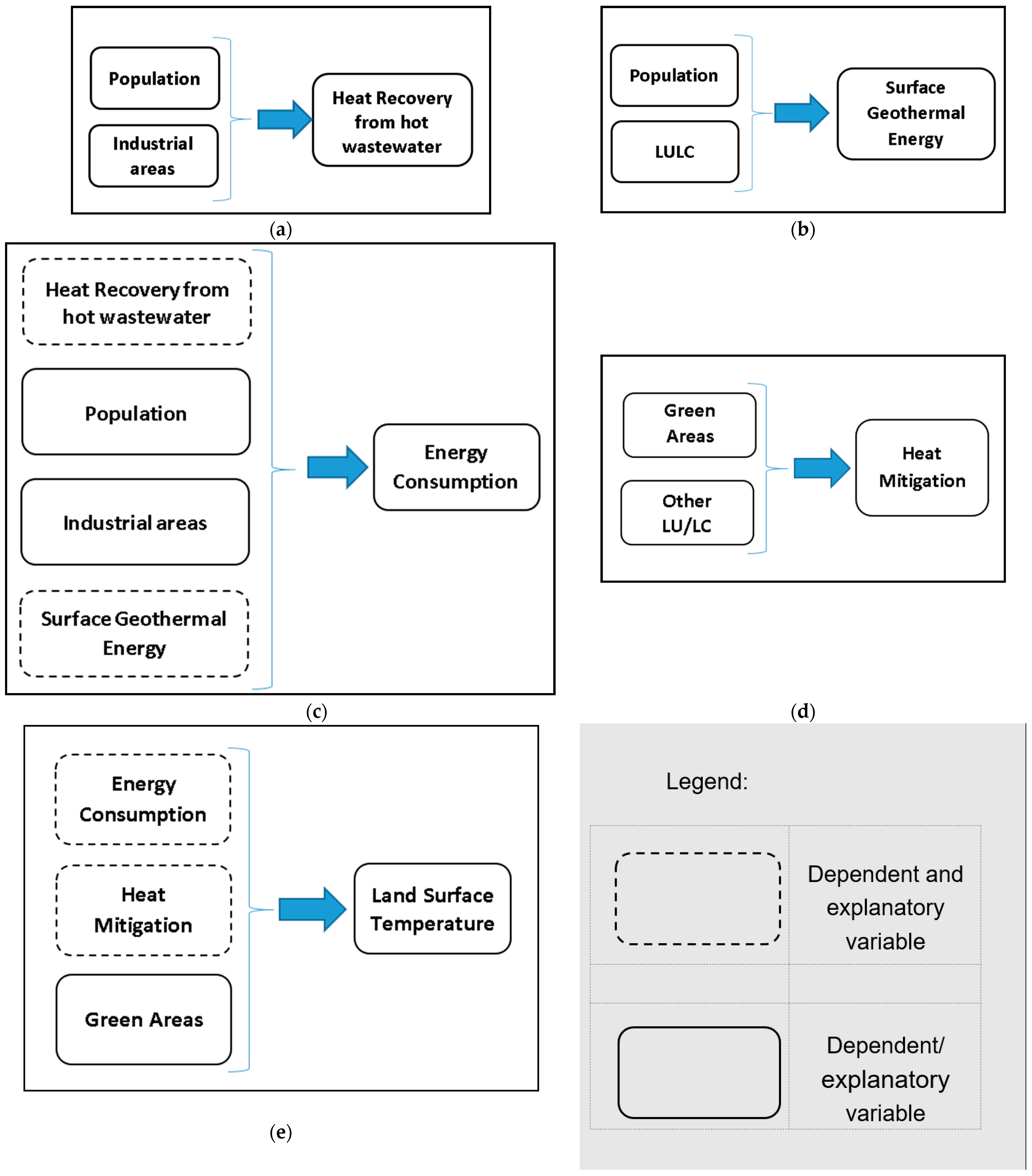
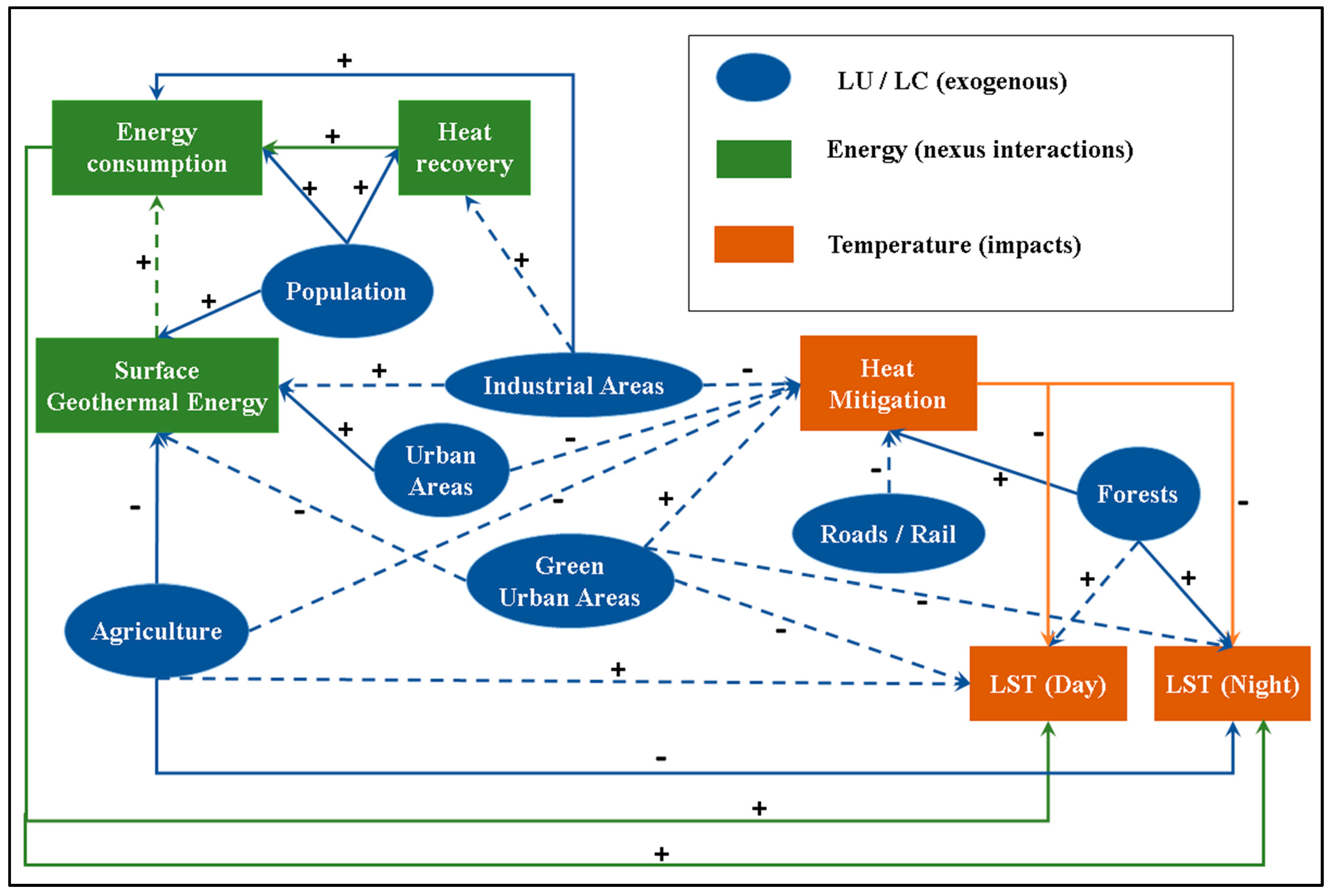
Along the same lines and starting with the first part of identifying the possible explanatory variables, a structure of logical relationships is proposed to be analyzed. For instance, the wastewater HR and the SGE were hypothetically supposed to affect the EC in addition to the area of industrial land use and the demographic population. It is also hypothesized that the HR from wastewater is highly dependent on population and industrial areas where most of the hot wastewater is generated. It is also supposed that the SGE, which is usually implemented in the gardens of individual homes, is highly dependent on population and land use type. By way of explanation, the estate prices in industrial areas are usually less than in other urban zones. Moreover, the green areas were also supposed to affect the HM capacity of spatial zones, which could, in turn, affect the land surface temperature (LST) in addition to the consumption of energy and the areas of green zones. Figure 4 shows a structure of relationships between the aforementioned factors.

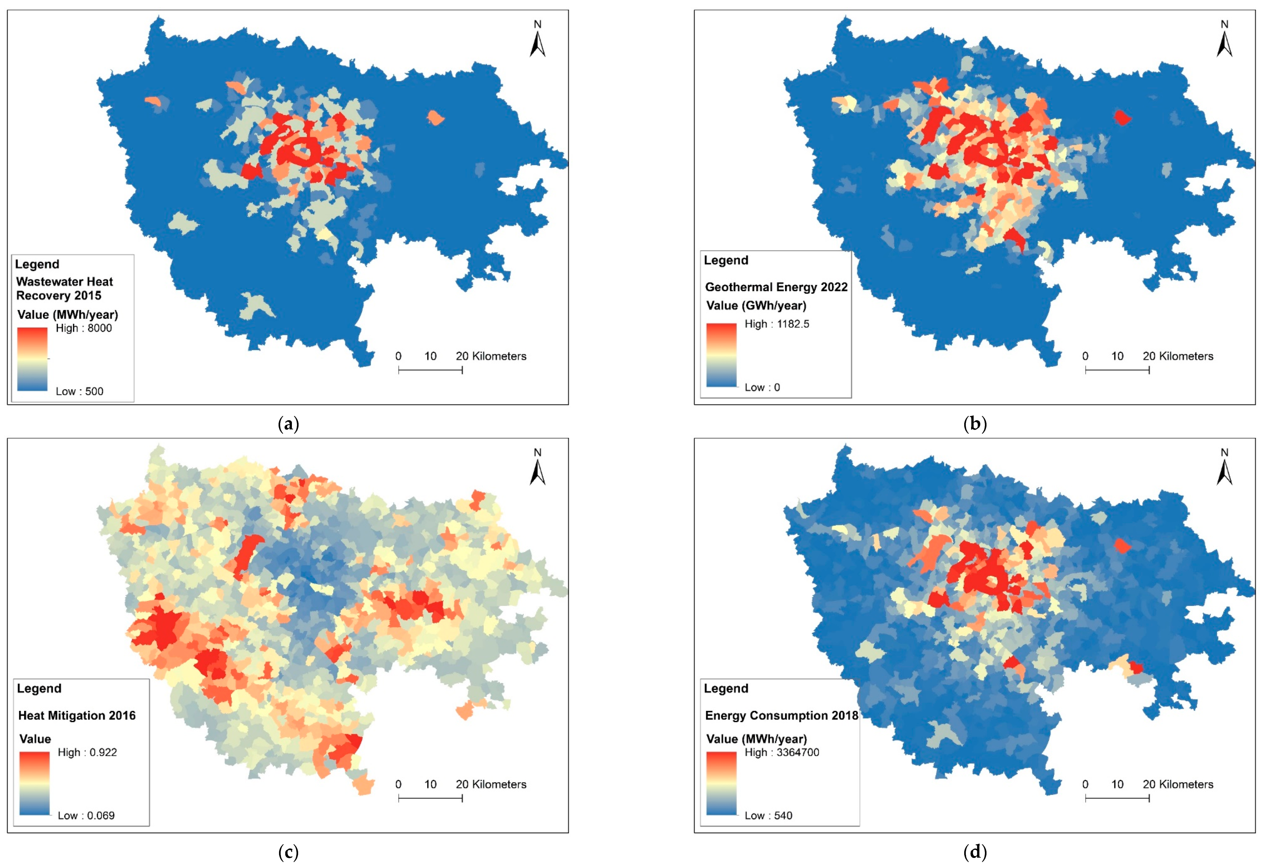
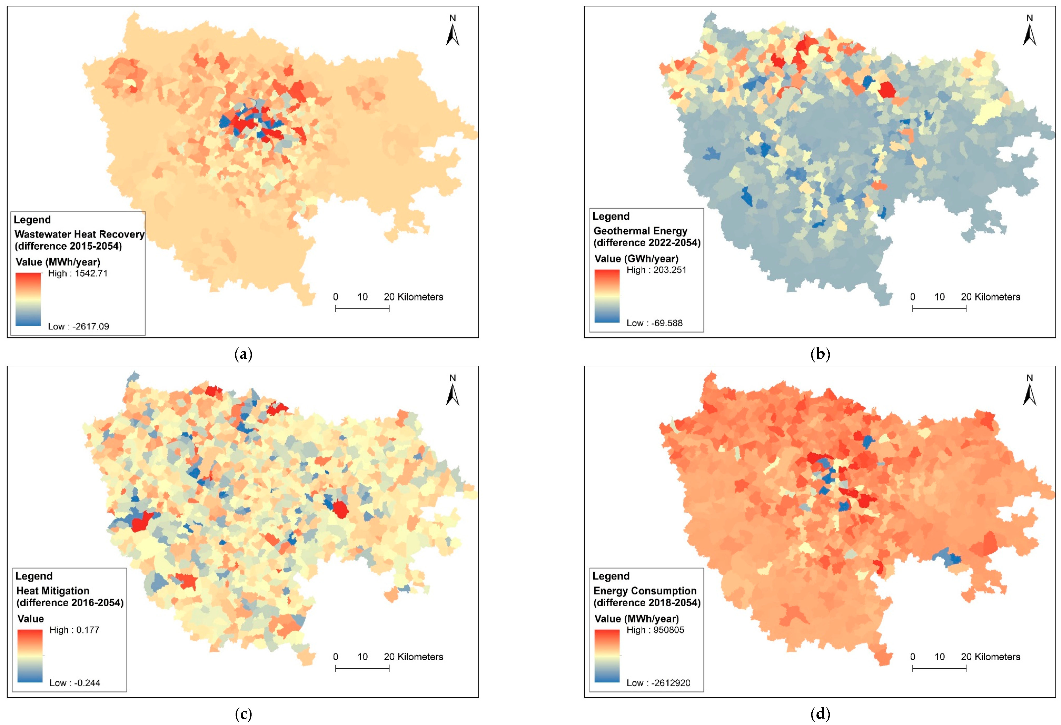
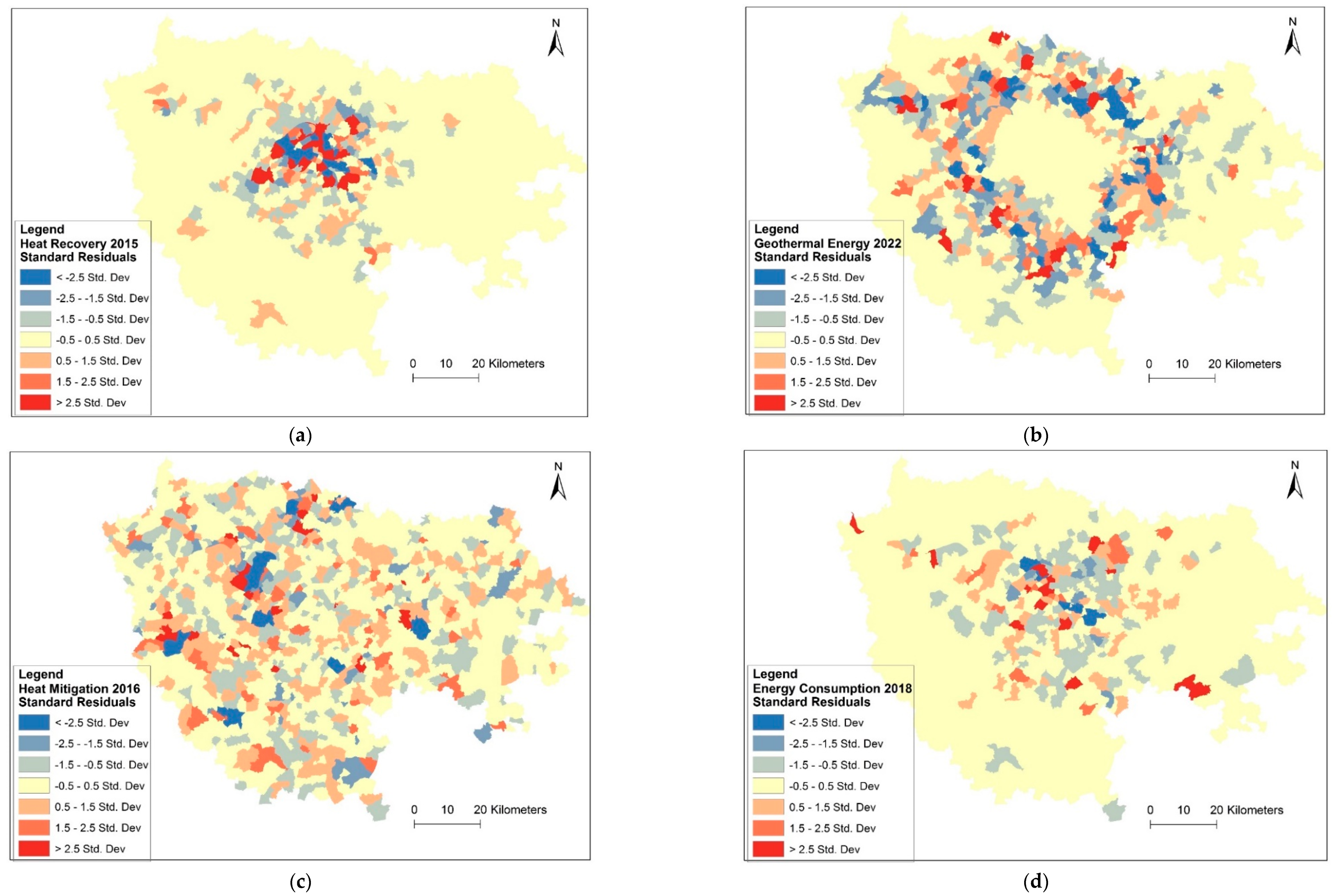
Accordingly, the data of (i) population, (ii) land use/land cover (LULC), (iii) SGE, (iv) HM index, (v) EC, (vi) HR from hot wastewater, and (vii) LST index were collected from different sources. The data of population for the year 2017 were collected from the population database of INSEE (2021) website. The Urban Atlas [36] provides the LULC maps for the Île-de-France area for the years 2006, 2012, and 2018. The data on wastewater heat recovery for the year 2015 indicates a concentric form of high capacities at the center with low capacity for the neighboring suburban areas. 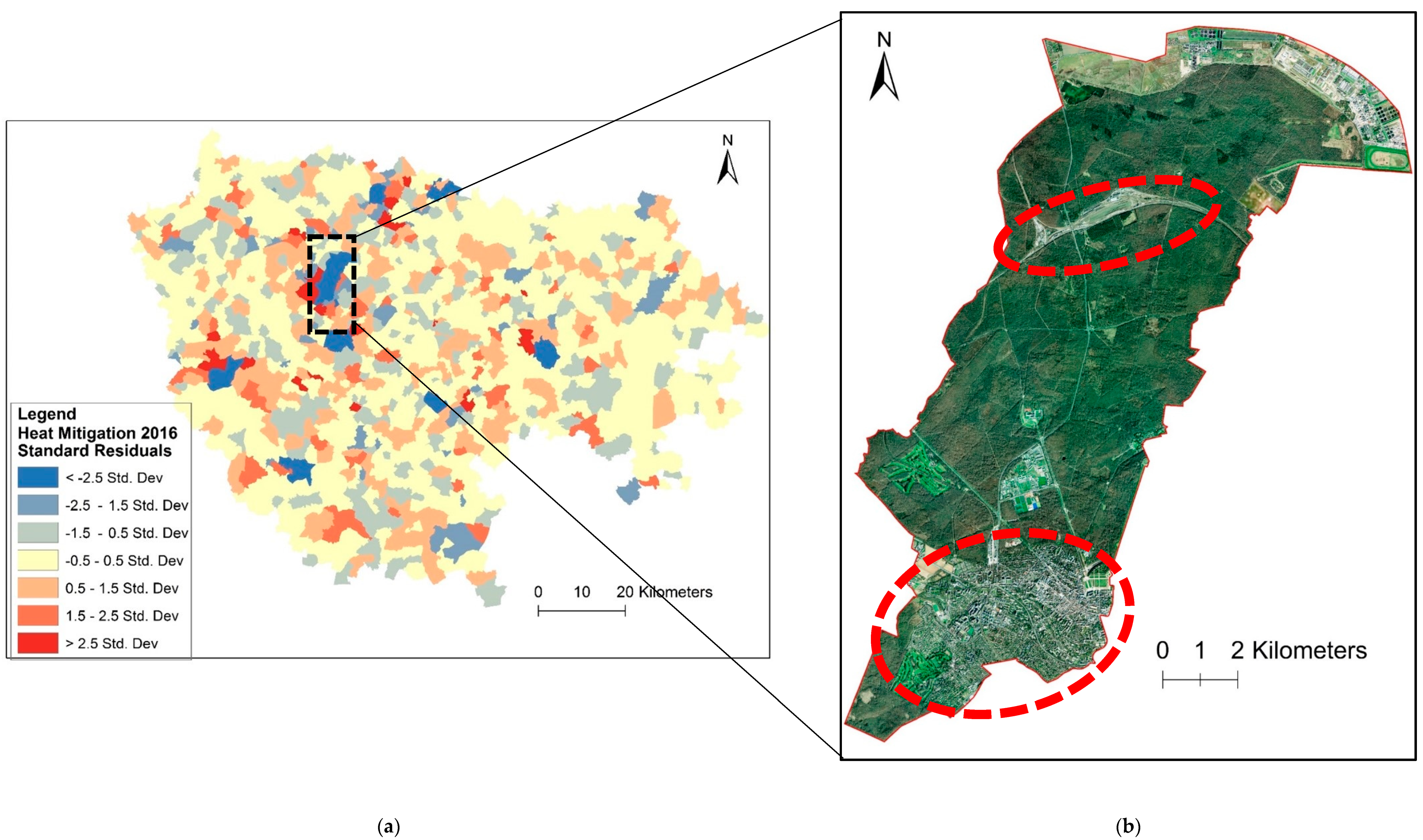The potential of SGE available only for a small area in the Île-de-France region in the year 2022 was collected by digitizing the published distribution map of the Bureau de Recherches Géologiques et Minières [33]. In the same context, it is important to note that the data of SGE was extended by conducting a regressing projection of the ordinary least square (OLS) to cover the whole study area. The pattern of these data is mostly a ring and extends slightly to neighboring areas where the existence of many individual homes with private gardens where the SGE systems could be installed. The HM indexes for the Île-de-France region for the year 2016 were collected in a rasterized form from the Naturvation project [10]. These values were aggregated, by average, to the community’s level. The pattern of these data follows that of the distribution of forests. 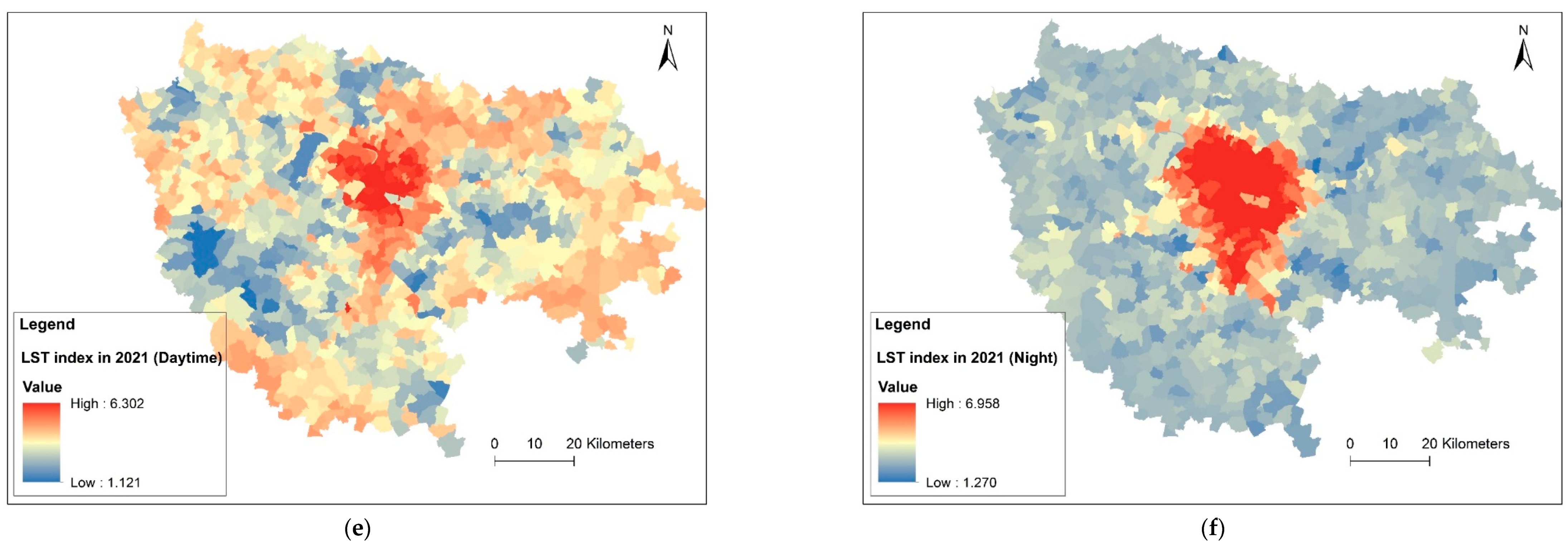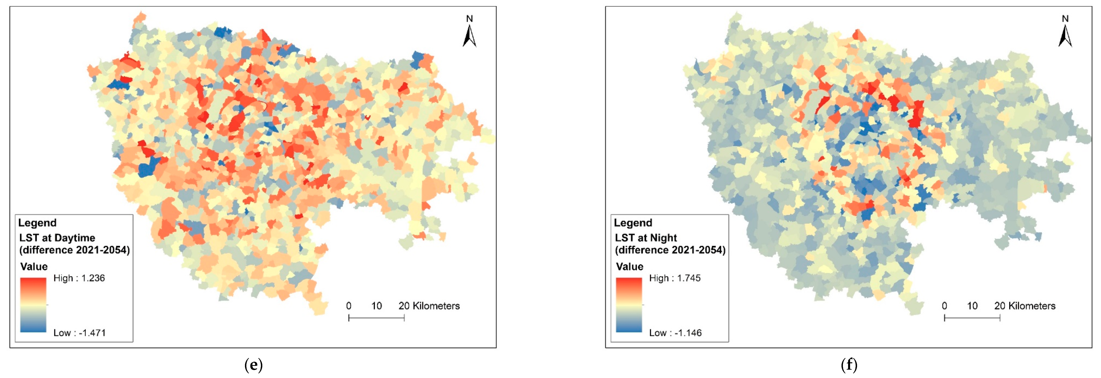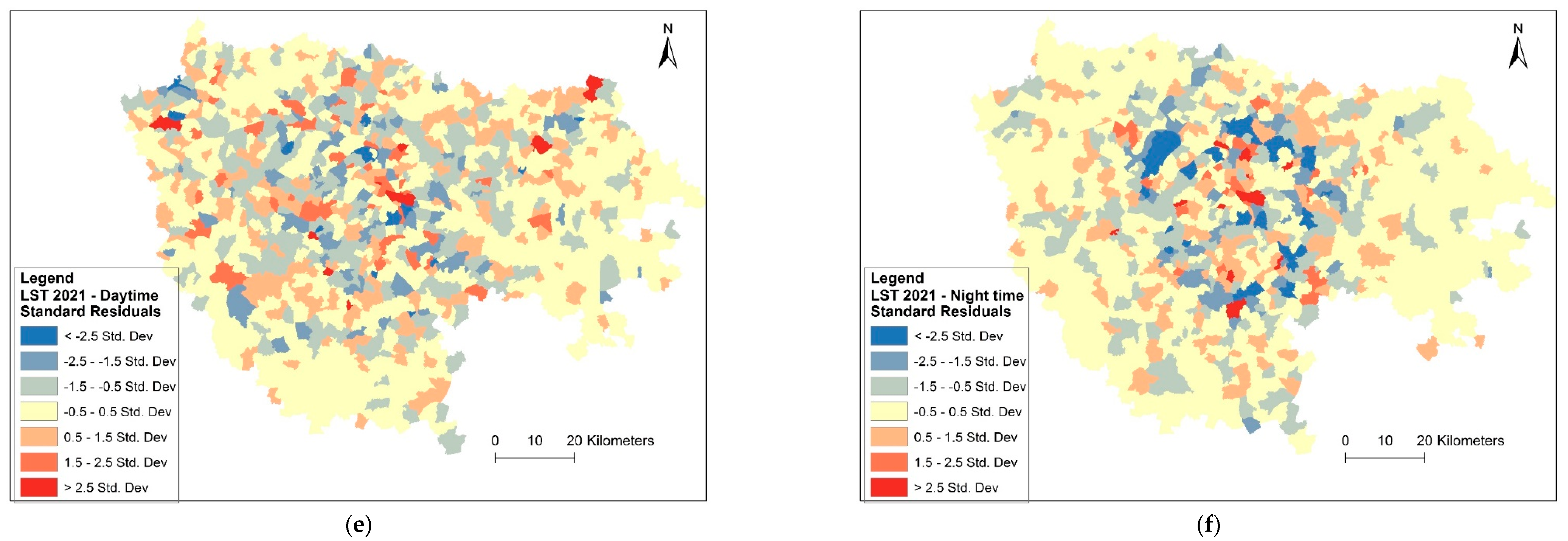The available data of EC for the year 2018, as well as that of HR from hot wastewater for the year 2015 in the Île-de-France region, were collected from the website of the Réseau d’Observation Statistique de l’Énergie [5]. The EC pattern shows a downward radial trend of distribution from high values at the center to low values in peripheral areas. The land surface temperature indexes for the year 2021 were collected from the “Ilots de Chaleur Urbains” data provided by Institut Paris Région [37]. The texture of the distribution of LST indexes during daytime is almost the opposite of that of HM. Similar to the EC pattern, the distribution of LST indexes at night follows a downward path of distribution from high indexes in the center to low indexes at the fringes. Figure 5 presents the maps of the collected data.

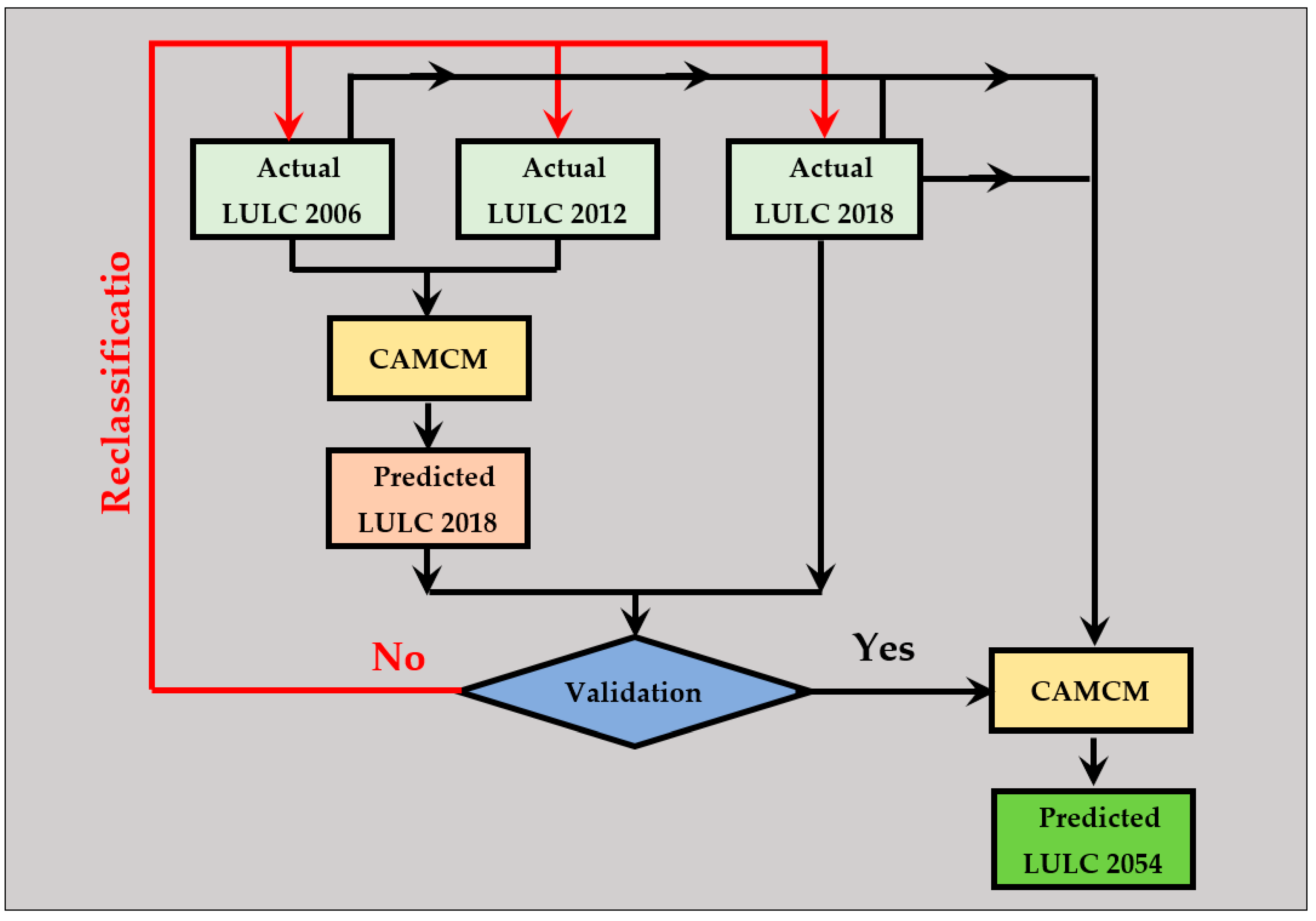
The LULC maps of the years 2006, 2012, and 2018 were used to predict the LULC for the year 2054 using the Cellular Automata Markov Chain Model (CAMCM). The time span of the prediction is 36 years and is commonly used in the scientific literature for LULC predictions mainly because 36 is a multiple of 12 (the period extended between the years 2006–2018) and because it constitutes a relatively long-term horizon. The first phase of this prediction process is the validation of the data used. This is conducted by (a) employing the available mapped data of 2006 and 2012 to predict the LULC for the year 2018 via the CAMCM simulations performed in TerrSet 18 software, and by (b) comparing the actual and predicted LULC maps for the year 2018. The prediction model was validated through Cohen’s kappa test conducted in TerrSet 18. The validation process showed high accuracy values of the predicted LULC for the year 2018. For instance, the calculated kappa values were all above 98%, indicating an almost perfect prediction according to Al-Shaar et al. [38]. In detail, the kappa values were 0.9919 for “Kappa for no information (Kno)”, 0.9955 for “Kappa of grid cells level location (Klocation)”, 0.9999 for “Kappa of stratum level location (KlocationStrata)” and 0.9896 for the “Overall kappa (Kstandard)”. Subsequently, the LULC maps of the years 2006 and 2018 were the inputs to predict the LULC for the year 2054. Figure 6 shows the process of predicting the LULC maps for the year 2054.

The changes of LULC between the years 2018 and 2054 showed (a) an increase of 5.52%, 17.7%, 1.25%, and 5%, respectively, in urban areas, industrial areas, forest, and wetlands, and the total area of roads and rail services; and (b) a decrease of 1.39%, 4.4%, and 50.9%, respectively, in the green urban areas, agriculture lands and bare soil zones. The land use/land cover distributions for the years 2018 and 2054 are presented in Figure A1 and Figure A2 in Appendix A. The population data for the year 2054 were calculated based on the forecasts in Île-de-France, which were prepared by INSEE [39]. The population in Île-de-France for the year 2013 was 11,959,800 persons [39]. These forecasts show that the population in Île-de-France in the year 2050 will be 13,504,900 persons. A simple projection for the year 2054 was conducted and indicated a population size of 13,689,488 persons.

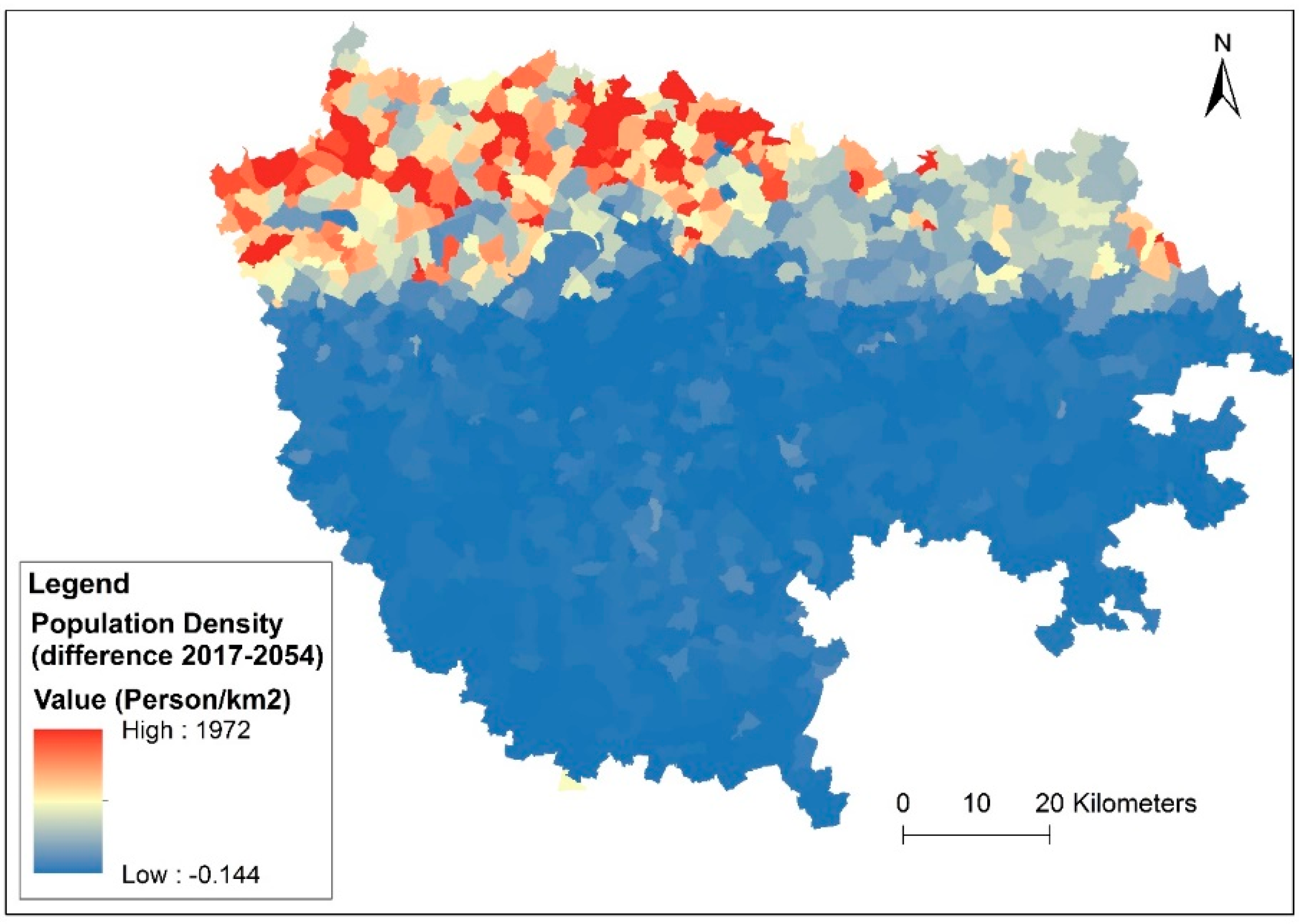
The population growth amounts in the study area communities are considered proportional to the urban growth rate in each community indicated by the predicted LULC distribution for the year 2054. Accordingly, the changes in population density between the years 2017 and 2054 show strong population growth in the North and Northeast of the study area. These changes are presented in Figure 7.

The current and projected data (to the year 2054) of population and LULC distributions are used in the statistical models, especially the GWR and ANOVA, to predict the evolution of SGE, hot wastewater HR and EC as well HM index, in addition to land surface temperature index.

3. Models Developed

This Section presents the findings obtained from the correlation analysis, the used OLS and GWR regression models, the spatial autocorrelation, and the variance analyses.

3.1. Correlation Analysis

The correlation analysis, which was carried out with R software, represents the refinement phase of the used data. This analysis is applied to support the following “selection of variables” phase by indicating what collinear variables could be reduced. This simplification is operated by keeping one representative variable and removing the remaining among the observed collinear variables. For instance, among the values of “carbon storage”, “stormwater retention index”, and HM index, only the HM index is used as one of the exploratory factors of dependent variables since the three aforementioned variables are all inter-correlated. It is important to indicate that the selection of the representative variable was performed based on several trials with the help of models used for the selection of variables, as indicated in the next sub-section. The correlation matrix, generated in R software, is presented in Figure A3 in Appendix B.

3.2. Selection of Variables

Ordinary Least Squares

The OLS regression model is the model used to select the variables. A derived OLS module called the exploratory regression (ER) was developed in ArcMap software. The ER runs all OLS models to cover all possible combinations of the explanatory variables, representing the input of the model. This ER model carried out in ArcMap 10.8 software indicates the coefficients of determination (R²) for all combinations. The selected model is the one having the highest R² with the least number of variables. All the selected models have an R² above 70% except the HM and the night LST models, with 62% and 60%, respectively. In the second stage, the OLS regression is applied to the selected model to determine the variance inflation factor (VIF) for each variable as well as for the overall model. Checking the values of VIF is necessary to ensure that there is no problem of multicolinearity. All the VIF values of the selected models are less than 10, which indicates no multicolinearity problems [35]. The spatial autocorrelation analysis was carried out as the final stage of this process to check whether the GWR approach is needed. The Moran’s I indexes ranged from 0.101 to 0.717, showing that the standard residuals are spatially auto-correlated. The z-scores of the spatial autocorrelations are all above 1.96, indicating the significance of the spatial autocorrelation (p-values < 0.05).

Table 1. Selected variables and summary of ordinary least squares results.

Model	Used Variables		Adjusted R2	Overall VIF	Residual Spatial Autocorrelation (p-Value)	Z-Score	Moran’s I coefficient
	Variables	VIF
Heat recovery from wastewater (year 2015)	Population 2017	3.21	0.75	1.3	<0.05	7.16	0.101
	Industrial areas 2018	2.01
Surface Geothermal Energy (year 2022)	Population 2017	1.91	0.72	1.88	<0.05	2.58	0.286
	Urban areas 2018	1.86
	Green Urban areas 2018	1.28
	Agriculture areas 2018	1.45
	Industrial areas 2018	1.45
Energy Consumption (year 2018)	Population 2017	6.06	0.84	6.15	<0.05	16.62	0.228
	Industrial areas 2018	1.74
	Heat recovery from wastewater 2015	4.24
	Surface geothermal energy 2022	6.17
Heat Mitigation (year 2016)	Urban areas 2018	2.23	0.62	3.32	<0.05	36.66	0.538
	Industrial areas 2018	3.03
	Roads and rail 2018	3.32
	Green urban areas 2018	1.44
	Forests 2018	1.10
	Agricultural areas 2018	1.17
Daytime Land Surface Temperature (year 2021)	Heat mitigation 2016	2.65	0.79	2.65	<0.05	38.52	0.566
	Energy consumption 2018	1.81
	Green urban areas 2018	1.40
	Forests 2018	2.40
	Agricultural areas 2018	1.27
Nighttime Land Surface Temperature (year 2021)	Heat mitigation 2016	2.65	0.60	2.65	<0.05	48.79	0.717
	Energy consumption 2018	1.81
	Green urban areas 2018	1.40
	Forests 2018	2.40
	Agricultural areas 2018	1.27

presents the selected variables and summarizes the results of OLS models.

3.3. GWR Models (Consistency and Prediction Power)

After checking the exogenous determining factors and the best combination models via the OLS models, the GWR regressions were applied to determine the values of regression relationships between the dependent variables and the driving variables according to their spatial distribution and local variations. The spatial features were taken into account individually. The regression coefficients calculated for the actual observations were afterward employed to conduct the projection for the year 2054 (using the LULC and population data of 2054). All the selected models have an R² above 83%.

The Moran’s I indexes ranged from 0.025 to 0.250, showing that residual spatial autocorrelation is still present. However, the Moran’ I coefficients are much lower, especially when data cover the whole area, such as that of SGE and HM.

The z-scores of the spatial autocorrelations are all above 1.96, indicating the significance of the spatial autocorrelation (p-values < 0.05) except for the data of SGE having a z-score of 1.75 corresponding to a significant p-value of 0.08.

Table 2. Coefficient of determination and spatial autocorrelation results of GWR models.

Model	Adjusted R2	Residual Spatial Autocorrelation (p-Value and Z-Score)	Moran’s I coefficient	Ratio: Moran’s I (OLS)/Moran’s I (GWR)
Surface geothermal energy 2022	0.987	(Z = 1.75, p = 0.08)	0.025	11.44
Energy consumption 2018	0.851	(Z = 12.65, p < 0.05)	0.172	1.33
Heat recovery from wastewater 2015	0.898	(Z = −3.13, p < 0.05)	−0.046	−2.20
Heat mitigation 2016	0.832	(Z = 3.53, p < 0.05)	0.051	10.55
Daytime LST intensity 2021	0.879	(Z = 11.72, p < 0.05)	0.172	3.29
Nighttime LST intensity 2021	0.898	(Z = 17.05, p < 0.05)	0.250	2.87

summarizes the results of GWR models as the coefficients of determination and spatial autocorrelation indicators.

Regarding the residuals of Wastewater HR, the pattern of their distribution is a central shape located in and around Paris. This distribution shows several under and over-estimations, which could be explained as the lack of explanatory variables described by the local regulations corresponding to HR and a

For the SGE, the residuals are distributed, with under and over-estimations, in the suburbs around the center of the studied area, not located on fringes, which are characterized by the individual type of residences, such as individual homes with gardens.

For HM, the existence of forests is not fully sufficient. The continuity of the forests was found to be an important factor that could determine the accuracy of estimating the HM capacity of the zone. For instance, the HM capacity of the Saint-Germain forest was underestimated by the GWR model. This could refer to the fact that some areas in this forest are employed for some urban activities, such as the railroad terminal/train depot indicated in Figure 8a,b. Similarly, the EC were under and overestimated in a radial form from the center to the peripheries. For instance, the EC was overestimated in the community of Grandpuits because of the existence of a no longer functioning oil refinery (the red spot in the southeastern part of the study area, as shown Figure A4 in Appendix C). The underestimation of the nighttime LST index is concentrated around the center. In addition, the GWR model under and overestimated the nighttime LST in a dispersed radial form to peripheries (Figure A4 in Appendix C). It is worth noting that the HM and the existence of forests are not fully sufficient for GWR estimations (for instance, in the Saint-Germain forest, where some human activities such as the train terminal exist, the GWR underestimated the LST index at night time). These findings reveal the need to integrate additional data that could enhance the estimations and increase accuracy. The spatial distribution pattern of residuals for the estimated daytime LST index is random with slight under/overestimation. This indicates that estimations are nearly correct. Figure 8a illustrates the spatial distribution of standard residuals for the HM GWR model. The mapped residual distributions of GWR models are illustrated in Figure A4 in Appendix C.

3.4. Effect Size (Variance Analysis)

The variance analysis was carried out to identify the effect size of determining factors for each dependent variable. The effect size is calculated as the ratio of the “sum of squares” for each determining variable to the total of the “sum of squares” of all determining factors. The analysis shows that population is the main determining factor for HR, with a percentage of 99.66; the industrial areas have a slight effect. Regarding the SGE, the population is the factor having the most effect on power, with a percentage of 72.12. Urban areas and agriculture zones are the factors having medium to low effect powers, with percentages of 12.4 and 9.52, respectively. Population, HR, and industrial areas are the main factors affecting energy consumption, with percentages of 39.3, 33.19, and 24.61, respectively. The HM is mainly affected by the existence of forests, with a percentage of 86.02. With respect to the LST, the determining factors depend on the time of the day. While the HM and the EC are the main determining factors for LST in the daytime with percentages of 85.66 and 8.20, respectively, the LST at night is affected by HM, EC, the existence of agriculture areas and forests with percentages of 22.84, 35.38, 31.6 and 8.93, respectively. It is worth mentioning here that from day to night times, the effect of heat mitigation is reduced by around 63%, which is distributed as an increase in the effect of (i) energy consumption by 27%, (ii) agriculture areas by 29%, and (iii) forest by 9%. The effects of determining factors support the selection of solutions and plans as well as supporting and guiding the enactment of corresponding policies. This change of effects between day and night times needs to be further investigated to identify the reasons behind them.

Table 3. The effect size of determining factors.

Model	Used Variables
	Variables	Effect Size (%)
Heat recovery from wastewater	Population 2017	99.66
	Industrial areas 2018	0.34
Surface geothermal energy	Population 2017	72.12
	Urban areas 2018	12.40
	Green urban areas 2018	2.60
	Agriculture areas 2018	9.52
	Industrial areas 2018	3.36
Energy consumption	Population 2017	39.30
	Industrial areas 2018	24.61
	Heat recovery from wastewater 2015	33.19
	Surface geothermal energy 2022	2.90
Heat mitigation	Urban areas 2018	3.40
	Industrial areas 2018	0.79
	Roads and rail 2018	0.72
	Green urban areas 2018	4.22
	Forests 2018	86.02
	Agricultural areas 2018	4.85
Daytime land surface temperature	Heat mitigation 2016	85.66
	Energy consumption 2018	8.20
	Green urban areas 2018	3.93
	Forests 2018	0.07
	Agricultural areas 2018	2.14
Nighttime land surface temperature	Heat mitigation 2016	22.84
	Energy consumption 2018	35.38
	Green urban areas 2018	1.25
	Forests 2018	8.93
	Agricultural areas 2018	31.60

presents the effect sizes of GWR determining factors.

Figure 9 shows the regression relationship structure among all dependent and exogenous variables. Effect sizes below 5% are indicated by disconnected lines in the regression relationship structure. Positive and negative regression relationships are indicated respectively by the signs of “+” and “−”.

4. Results and Discussion

The predicted EC pattern for the year 2054 generally shows an increasing trend in the whole area, especially in the north and northwest part of the study area, where concentrated population growth occurs. It is worth noting that in some areas in proximity to the central zone, the energy consumption is expected to be reduced. This could refer to the individual behavior of reducing energy consumption and/or the effects of policies or other unidentified factors.

On the other hand, the expected potentials for HR and SGE are not in line with the forecasted EC, particularly in the southwest and southeast parts of the central zone and its neighboring areas. In these two zones, the potential to recuperate heat energy is lowered compared to the current period. In contrast, in other zones, the expected potentials for HR and SGE are compatible with the needs for the forecasted EC. For instance, the HR is expected to increase in the northern part of areas surrounding the center. Similarly, the SGE is expected to increase in the north and northwest parts of peripheral zones in the study area. A third important case of energy supply versus demand is notable. It is depicted, as in the case where the potential to recuperate energy from wastewater is high, nonetheless, the energy consumption is reduced. This forecast is expected in some areas of Paris where the HR will be intensified due to possible regulations or implementation of HR systems and accompanied by a decrease in energy consumption. The predicted changes in HM capacities between the years 2016 and 2054 show different increased and decreased values. What is important to point out is that some of the reduced capacities are accompanied by an increase in population density (2017–2054) such as in the northwest region of the study area. However, the reduced capacities of HM observed in the remaining areas that are not associated with new human settlements need to be further investigated, in future research, to identify the main causes of these predicted changes.

The texture of the distribution of the predicted LST indexes during the daytime is almost the opposite of that of HM. Similar to the EC pattern, the predicted distribution of LST indexes at night follows a downward path of distribution of high indexes at the center to low indexes at the fringes. Figure 10 shows the predicted change of (a) wastewater heat recovery (2015–2054); (b) surface geothermal energy (2022–2054); (c) heat mitigation (2016–2054); (d) energy consumption (2018–2054); (e) daytime LST (2021–2054); and (f) night time LST (2021–2054).

5. Conclusions

This paper investigates the trends and the solutions to manage the water–soil–energy nexus in the context of increasing urbanization. The examined solutions, integrated into the water–soil–energy nexus, are designed primarily to reduce the consumption of fossil energy by discovering and implementing new renewable sources of energy and for heat mitigation by examining the spatial possibilities for afforestation/reforestation. However, the effects of exogenous spatial driving factors of these solutions, in addition to their future spatial evolution are not holistically studied. Bearing in mind the spatial competition between different land use/land cover patterns, the analysis is elaborated by (a) determining the areas with low, medium, and high potential for implementing the solutions, as well as defining the type of solution to be implemented, and (b) by comparing the aforementioned implementation capacities with the demand depicted as the needs for slowing down the effects of the surface urban heat islands and warming, and reducing dependence on fossil energy. This study identifies the current key drivers of the SGE, the wastewater HR and the spatial capacity for HM in the study area, which covers a wide spatial extent in the Île-de-France region, in addition to their potential spatial changes until the year 2054. This methodology used the statistical analysis of OLS and GWR, combined with the geographic information system, based on data on land use/land cover as well as the distribution of population. The findings indicate that the spatial autocorrelation of GWR residuals is lesser than those of OLS models. The difference, introduced as the ratios, ranges from 1.33 to 11.44. These values are clearly observed particularly in the cases of SGE (11.44) and HM (10.55). On that account, GWR models explain the regressive relationships between key drivers and WSE solutions at the individual spatial level. In addition, these models predict the spatial evolution of the examined WSE solutions. In addition, variance analyses were conducted to quantify the influence of each driving factor. For instance, and with respect to LST, the key determinants change over the daytime. Whereas the HM and the EC are the main determining factors for daytime LST with effect sizes of 85.66% and 8.20%, respectively, the nighttime LST is affected by HM and EC in addition to the existence of agriculture areas and forests with effect sizes of 22.84%, 35.38%, 31.6%, and 8.93%, respectively. This change needs to be further investigated to identify the reasons behind it since the effects of determining factors support the selection of solutions and plans as well as supporting and guiding the enactment of corresponding policies. Regarding the prediction results, areas with the potential for implementing specific solutions are determined and classified according to their capacities. Along the same lines, these capacities are compared to the demand for reducing the dependence on fossil energy and slowing down the effects of surface urban heat islands. The predictions indicate three types of distribution regarding the energy consumption: (i) the best fit where the potential for implementing SGE or HR is elevated and associated with an increase in energy consumption as in the northern part of areas surrounding the center of Île-de-France, (ii) the medium pattern where the potential for implementing SGE or HR is elevated, however, the energy consumption is expected to decrease as in some area of Paris, and (iii) the worst case where the potential for implementing SGE or HR is low/null and the energy consumption is expected to increase as in the southwest and southeast parts of the central zone and its neighboring areas. With respect to the predicted change of HM capacities between the years 2016 and 2054, it is important to mention that in some areas the forecasted reduced capacities of HM are not associated with human activities. The reasons behind this change should be clarified by further research. Concerning the limitations, the solutions designed (a) to mitigate the risk of climate change, floods, air pollution, and temperature, (b) to protect biodiversity, and (c) to reduce the dependence on fossil energy, such as the green roofs and vegetated facades as well as the solar energy, were not inspected due to limited data and information about the explanatory variables.

Moreover, the impacts of air temperature on the consumption of fossil energy were not investigated. It would be interesting to clarify all these points in further research.

References

1. Ferreira, V.; Barreira, A.P.; Loures, L.; Antunes, D.; Panagopoulos, T. Stakeholders’ Engagement on Nature-Based Solutions: A Systematic Literature Review. Sustainability 2020, 12, 640. [Google Scholar] [CrossRef] [Green Version]
2. Directorate-General for Research and Innovation (European Commission). Towards an EU Research and Innovation Policy Agenda for Nature-Based Solutions & Re-Naturing Cities: Final Report of the Horizon 2020 Expert Group on ’Nature Based Solutions and Re Naturing Cities; Publications Office of the European Union: Brussels, Belgium, 2015; ISBN 978-92-79-46051-7. [Google Scholar]
3. Dick, J.; Miller, J.D.; Carruthers-Jones, J.; Dobel, A.J.; Carver, S.; Garbutt, A.; Hester, A.; Hails, R.; Magreehan, V.; Quinn, M. How Are Nature Based Solutions Contributing to Priority Societal Challenges Surrounding Human Well-Being in the United Kingdom: A Systematic Map Protocol. Environ. Evid. 2019, 8, 37. [Google Scholar] [CrossRef] [Green Version]
4. World Bank. World Bank Biodiversity, Climate Change, and Adaptation: Nature-Based Solutions from the World Bank Portfolio; World Bank: Washington, DC, USA, 2008. [Google Scholar]
5. Réseau D’observation Statistique de L’énergie (ROSE). Energif|Consommations Enérgétiques Détaillées du Secteur Résidentiel. Available online: http://sigr.iau-idf.fr/webapps/cartes/rose/?op=d (accessed on 18 May 2022).
6. Stober, I.; Bucher, K. Geothermal Energy: From Theoretical Models to Exploration and Development; Springer International Publishing: Cham, Switzerland, 2021; ISBN 978-3-030-71684-4. [Google Scholar]
7. Naili, N.; Hazami, M.; Attar, I.; Farhat, A. Assessment of Surface Geothermal Energy for Air Conditioning in Northern Tunisia: Direct Test and Deployment of Ground Source Heat Pump System. Energy Build. 2016, 111, 207–217. [Google Scholar] [CrossRef]
8. Saagi, R.; Arnell, M.; Wärff, C.; Ahlström, M.; Jeppsson, U. City-Wide Model-Based Analysis of Heat Recovery from Wastewater Using an Uncertainty-Based Approach. Sci. Total Environ. 2022, 820, 153273. [Google Scholar] [CrossRef]
9. Spriet, J.; McNabola, A.; Neugebauer, G.; Stoeglehner, G.; Ertl, T.; Kretschmer, F. Spatial and Temporal Considerations in the Performance of Wastewater Heat Recovery Systems. J. Clean. Prod. 2020, 247, 119583. [Google Scholar] [CrossRef]
10. NATure-Based URban innoVATION Project (Naturvation) European Assessment Maps. Available online: https://naturvation.eu/assessment/maps (accessed on 7 March 2022).
11. Sowińska-Świerkosz, B.; García, J. What Are Nature-Based Solutions (NBS)? Setting Core Ideas for Concept Clarification. Nat. Based Solut. 2022, 2, 100009. [Google Scholar] [CrossRef]
12. Blackwood, L.; Renaud, F.G.; Gillespie, S. Nature-Based Solutions as Climate Change Adaptation Measures for Rail Infrastructure. Nat. Based Solut. 2022, 2, 100013. [Google Scholar] [CrossRef]
13. Pander, J.; Mueller, M.; Geist, J. Succession of Fish Diversity after Reconnecting a Large Floodplain to the Upper Danube River. Ecol. Eng. 2015, 75, 41–50. [Google Scholar] [CrossRef]
14. Schindler, S.; O’Neill, F.H.; Biró, M.; Damm, C.; Gasso, V.; Kanka, R.; van der Sluis, T.; Krug, A.; Lauwaars, S.G.; Sebesvari, Z.; et al. Multifunctional Floodplain Management and Biodiversity Effects: A Knowledge Synthesis for Six European Countries. Biodivers. Conserv. 2016, 25, 1349–1382. [Google Scholar] [CrossRef] [Green Version]
15. Funk, A.; Martínez-López, J.; Borgwardt, F.; Trauner, D.; Bagstad, K.J.; Balbi, S.; Magrach, A.; Villa, F.; Hein, T. Identification of Conservation and Restoration Priority Areas in the Danube River Based on the Multi-Functionality of River-Floodplain Systems. Sci. Total Environ. 2019, 654, 763–777. [Google Scholar] [CrossRef]
16. Perni, A.; Martínez-Paz, J.M. A Participatory Approach for Selecting Cost-Effective Measures in the WFD Context: The Mar Menor (SE Spain). Sci. Total Environ. 2013, 458–460, 303–311. [Google Scholar] [CrossRef]
17. Majidi, A.N.; Vojinovic, Z.; Alves, A.; Weesakul, S.; Sanchez, A.; Boogaard, F.; Kluck, J. Planning Nature-Based Solutions for Urban Flood Reduction and Thermal Comfort Enhancement. Sustainability 2019, 11, 6361. [Google Scholar] [CrossRef] [Green Version]
18. Soana, E.; Fano, E.A.; Castaldelli, G. The Achievement of Water Framework Directive Goals through the Restoration of Vegetation in Agricultural Canals. J. Environ. Manage. 2021, 294, 113016. [Google Scholar] [CrossRef]
19. Harrington, R.; O’Donovan, G.; McGrath, G. Integrated Constructed Wetlands (ICW) Working at the Landscape Scale: The Anne Valley Project, Ireland. Ecol. Inform. 2013, 14, 104–107. [Google Scholar] [CrossRef]
20. Benedict, M.A.; McMahon, E.T. Green Infrastructure: Smart Conservation for the 21st Century. Renew. Resour. J. 2002, 20, 12–17. [Google Scholar]
21. Liu, W.; Xu, H.; Zhang, X.; Jiang, W. Green Infrastructure Network Identification at a Regional Scale: The Case of Nanjing Metropolitan Area, China. Forests 2022, 13, 735. [Google Scholar] [CrossRef]
22. Seddon, N.; Chausson, A.; Berry, P.; Girardin, C.A.J.; Smith, A.; Turner, B. Understanding the Value and Limits of Nature-Based Solutions to Climate Change and Other Global Challenges. Philos. Transact. R. Soc. B Biol. Sci. 2020, 375, 20190120. [Google Scholar] [CrossRef] [Green Version]
23. European Commission. European Commission Sustainable Europe Investment Plan European Green Deal Investment Plan; European Commission: Brussels, Belgium, 2020. [Google Scholar]
24. Nagpal, H.; Spriet, J.; Murali, M.K.; McNabola, A. Heat Recovery from Wastewater—A Review of Available Resource. Water 2021, 13, 1274. [Google Scholar] [CrossRef]
25. Wärff, C.; Arnell, M.; Sehlén, R.; Jeppsson, U. Modelling Heat Recovery Potential from Household Wastewater. Water Sci. Technol. 2020, 81, 1597–1605. [Google Scholar] [CrossRef] [Green Version]
26. Schmid, F. Sewage water: Interesting heat source for heat pumps and chillers. In Proceedings of the HPT—Heat Pumping Technologies, Zürich, Switzerland, 22 May 2008. [Google Scholar]
27. Dürrenmatt, D.J.; Wanner, O. A Mathematical Model to Predict the Effect of Heat Recovery on the Wastewater Temperature in Sewers. Water Res. 2014, 48, 548–558. [Google Scholar] [CrossRef]
28. Cipolla, S.S.; Maglionico, M. Heat Recovery from Urban Wastewater: Analysis of the Variability of Flow Rate and Temperature in the Sewer of Bologna, Italy. Energy Proced. 2014, 45, 288–297. [Google Scholar] [CrossRef]
29. Kretschmer, F.; Simperler, L.; Ertl, T. Analysing Wastewater Temperature Development in a Sewer System as a Basis for the Evaluation of Wastewater Heat Recovery Potentials. Energy Build. 2016, 128, 639–648. [Google Scholar] [CrossRef]
30. Ivajnšič, D.; Kaligarič, M.; Žiberna, I. Geographically Weighted Regression of the Urban Heat Island of a Small City. Appl. Geogr. 2014, 53, 341–353. [Google Scholar] [CrossRef]
31. Wang, Z.; Fan, C.; Zhao, Q.; Myint, S.W. A Geographically Weighted Regression Approach to Understanding Urbanization Impacts on Urban Warming and Cooling: A Case Study of Las Vegas. Remote Sens. 2020, 12, 222. [Google Scholar] [CrossRef] [Green Version]
32. Eklipse. EKLIPSE Draft Document of Work: Energy Request; Eklipse Management Body: Leipzig, Germany, 2017; p. 43. [Google Scholar]
33. Bureau de Recherches Géologiques et Minières (BRGM). Grand Paris: Le Potentiel de la Géothermie de Surface Cartographié|BRGM. Available online: https://www.brgm.fr/fr/actualite/communique-presse/grand-paris-potentiel-geothermie-surface-cartographie (accessed on 19 June 2022).
34. Hutcheson, G.D.; Moutinho, L. Statistical Modeling for Management; Sage Publishing: Newbury Park, CA, USA, 2022; ISBN 978-0-7619-7011-8. [Google Scholar]
35. Loonis, V.; de Bellefon, M.-P. Handbook of Spatial Analysis; Insee—Eurostat: Montrouge, France, 2018; ISBN 978-2-11-139686-9. [Google Scholar]
36. Urban Atlas. Urban Atlas—Copernicus Land Monitoring Service. Available online: https://land.copernicus.eu/local/urban-atlas (accessed on 25 November 2021).
37. Institut Paris Region Ilots de chaleur Urbains (ICU): Classification des IMU en Zone Climatique Locale (LCZ), Aléas et Vulnérabilités à la Chaleur de Jour et de Nuit en Île-de-France. Available online: https://data-iau-idf.opendata.arcgis.com/datasets/ilots-de-chaleur-urbains-icu-classification-des-imu-en-zone-climatique-locale-lcz-al%C3%A9as-et-vuln%C3%A9rabilit%C3%A9s-%C3%A0-la-chaleur-de-jour-et-de-nuit-en-%C3%AEle-de-france/explore?location=48.671264,2.503150,9.00 (accessed on 20 August 2022).
38. Al-Shaar, W.; Adjizian Gérard, J.; Nehme, N.; Lakiss, H.; Buccianti Barakat, L. Application of Modified Cellular Automata Markov Chain Model: Forecasting Land Use Pattern in Lebanon. Model. Earth Syst. Environ. 2021, 7, 1321–1335. [Google Scholar] [CrossRef]
39. Institut National de la Statistique et des Etudes Economiques (INSEE) Les Résultats Des Recensements de La Population|Insee. Available online: https://www.insee.fr/fr/information/2008354 (accessed on 4 January 2022).
Figure 1. Water–soil–energy nexus. Source: own elaboration.
Urbansci 06 00081 g001
Figure 2. The selected study area.
Urbansci 06 00081 g002
Figure 3. The structure of the methodology used.
Urbansci 06 00081 g003
Figure 4. Structure of relationships between possible determining factors and dependent factors: (a) heat recovery from hot wastewater; (b) surface geothermal energy; (c) energy consumption; (d) heat mitigation; and (e) land surface temperature.
Urbansci 06 00081 g004
Figure 5. The mapped data of (a) wastewater heat recovery (2015); (b) surface geothermal energy (2022); (c) heat mitigation (2016); (d) Energy Consumption (2018); (e) daytime LST (2021); and (f) night time LST (2021).
Urbansci 06 00081 g005aUrbansci 06 00081 g005b
Figure 6. Process of predicting the LULC maps for the year 2054.
Urbansci 06 00081 g006
Figure 7. The predicted change of population density (2017–2054).
Urbansci 06 00081 g007
Figure 8. (a) Spatial distribution of standard residuals for the HM GWR model, (b) the Saint-Germain Forest (red circles show urban development and activities in the Saint-Germain Forest).
Urbansci 06 00081 g008
Figure 9. Regression relationship structure among all dependent and exogenous variables.
Urbansci 06 00081 g009
Figure 10. The predicted change of (a) wastewater heat recovery (2015–2054); (b) surface geothermal energy (2022–2054); (c) heat mitigation (2016–2054); (d) energy consumption (2018–2054); (e) daytime LST (2021–2054); and (f) night time LST (2021–2054).
Urbansci 06 00081 g010aUrbansci 06 00081 g010b