Article

Urban Expansion Simulated by Integrated Cellular Automata and Agent-Based Models; An Example of Tallinn, Estonia

Department of Geography, Institute of Ecology and Earth Sciences, Faculty of Science and Technology, University of Tartu, Vanemuise 46, 50410 Tartu, Estonia
*
Author to whom correspondence should be addressed.
Urban Sci. 2021, 5(4), 85; https://doi.org/10.3390/urbansci5040085
Submission received: 22 September 2021 / Revised: 22 October 2021 / Accepted: 26 October 2021 / Published: 1 November 2021

Abstract

:
From 1990 to 2018, built-up areas in Tallinn, Estonia’s capital city, increased by 25.03%, while its population decreased by −10.19%. Investigating the factors affecting urban expansion and modeling it are critical steps to detect future expansion trends and plan for a more sustainable environment. Different models have been used to investigate, predict, and simulate urban expansion in recent years. In this paper, we coupled the cellular automata, agent-based, and Markov models (CA–Agent model) in a novel manner to address the complexity of the dynamic simulation, generate heterogeneity in space, define more complicated rules, and employ the suitability analysis. In the CA–Agent model, cells are dynamic agents, and the model’s outcome emerges from cellular agents’ interactions over time using the rules of behavior and their decisions concerning the adjacent neighboring cells and probabilities of spatial changes. We performed the CA–Agent model run two times for 2018 and 2030. The first simulated results were used to validate the performance of the model. Kappa showed 0.86, indicating a relatively high model fit, so we conducted the second 12-year run up to the year 2030. The results illustrated that using these model parameters, the overall built-up areas will reach 175.24 sq. km with an increase of 30.25% in total from 1990 to 2030. Thus, implementing the CA–Agent model in the study area illustrated the temporal changes of land conversion and represented the present spatial planning results requiring regulation of urban expansion encroachment on agricultural and forest lands.

1. Introduction

Urban expansion is the process of conversion of lands to urban [1]. Shifts from agricultural lands [2,3,4], forest lands [5,6], water [7,8,9,10], and wetlands [6,11,12] are among the most critical transitions to urban lands. This causes adverse impacts on the physical environment and is one of the leading causes of natural ecosystem degradation [13]. It causes loss of the agriculture and croplands, habitat fragmentation, heat island effects, and reduction of surface watercourses [14,15,16]. It also causes changes in landscapes [17,18,19,20] and urban transportation needs by increasing travel distance and commuting trips between the city and suburbs, demand for private cars, and fuel consumption [21,22].
Land use/land cover (LULC) maps are the products of the classification of satellite remote-sensing images [23], which enable quantitative spatiotemporal analysis across geographic regions [24] and provide helpful information about the transformation of lands [25,26] to a temporal extent. Eventually, extracting urban areas from LULC maps and modeling provides a critical investigation into urban expansion’s driving mechanisms, future trends, and LULC transitions [27].
Since urban expansion is a dynamic and complex process, many spatial models have been constructed to investigate, predict, and simulate it. Simulation models can develop scenarios for future-oriented decision-making [28] by preparing a projection of land-use changes, expecting the future urban land demands and spatial distribution of these demands [29]. Among others, these models include the cellular automata (CA) model [30,31,32], CA–Markov model [33,34,35], logistic regression model [36,37,38], agent-based model [39,40] and multi-agent-based model [41,42]. Of these models, CA has been the most popular model employed by researchers since its conceptualization by Ulam and Von Neumann in the 1940s [43,44]. A countless number of studies on the application of CA in modeling urban expansion exist. For example, Ma et al. [45] attempted to examine CA to simulate urban expansion in China. Putting seed data and control layers, they explored the parameters for their model and reached high accurate simulation results. White et al. [46] employed the constrained CA model based on the development intensity or dynamic constraints in space and time to predict urban land-use dynamics. Mozaffaree Pour and Oja. [47] modeled urban expansion in Harju County in Estonia to investigate its driving forces and predict the future trend in a regular cell space.
Integrating CA with other models increased the popularity, efficiency, and quantity of the simulation [48] in the field of urban expansion. Integrated CA–Markov has been implemented in research, considering that the trend and pace of changes in the urban expansion are similar in the past and future. In a study performed by Li et al. [34], they explored the capabilities of CA–Markov to simulate urban expansion in China. Prediction of urban expansion employing the CA–Markov model in Iran was performed by Jafari et al. [49] and revealed expansion on the periphery of population centers with encroachment to the forest and agricultural lands. The integrated logistic–CA model was conducted in some research [50,51,52], exploring the spatial feature of urban expansion and defining transition rules. In the research by Mustafa et al. [50], they took advantage of multinominal logistic regression and CA to assess the probabilities of causative factors and neighborhood effects in the urban expansion of Belgium. To explore the relationships between land conversion and driving factors of urban expansion, Arsanjani et al. [52] employed integrated logistic–CA–Markov models to simulate land use maps consisting of built-up lands and calculate the quantity of land-use change using a transition area matrix in Tehran, Iran.
Furthermore, several studies enhanced the CA model with agent-based models to explore the drivers of urban expansion, boost the behavioral rules by defining the dynamic agents, and determine more realistic neighborhood effects to simulate urban expansion. Mustafa et al. [29] have considered a combination of CA–Logit and agent-based modeling to capture the dynamics of neighborhood interactions and static drivers of urban expansion in three levels of agents with homogeneous characteristics and behaviors. Liu et al. [53] constructed a land-use simulation and decision-support system (LandSDS), integrating agent-based and CA modeling in China for two homogeneous agents. However, models of urban expansion simulation vary in terms of data requirements, mechanisms, and application scales [48]; these models have limitations, and considerably new integrated model approaches are required to meet the complexity of urban expansion nature, which deal with spatial heterogeneity, local interactions, and neighborhood effects.
To this aim, we coupled the CA model with the agent-based model (CA–Agent model) to address the complexity of the dynamic simulation, generate heterogeneity in space, define more complicated rules, and employ the suitability analysis in a novel way.
Cellular automata as a bottom-up model is based on regular or irregular cell space depending on the complexity of the representation of reality [54] and consider the interactions between cells and their neighbors implemented by transition rules. Defining transition rules is the critical step in CA models. While transition rules are invariant through time [32], considering the spatial heterogeneity among the cells and uneven development in simulation requires improvements of transition rules [55]. Applying the appropriate thresholds is a way to address the spatial heterogeneity [56]. One of the key benefits of our CA–Agent model is implementing different transition rules manipulated by suitability thresholds for cellular agents.
Moreover, a heterogeneous neighborhood impacts the spatial heterogeneity [57] and the model simulation results. Taking advantage of the suitability analysis, we enhanced the CA–Agent model performance to simulate the most suitable areas for new areas expansions [39]. Eventually, the CA model is flexible with an adaptable structure capable of integrating with other models [58,59].
Additionally, agent-based models as generative simulation modeling [60] employ the behavioral factors of agents and their interactions with the environment and with one another to simulate the urban evolution [61] and track the dynamic changes from one agent to the whole area [62]. Agents could be defined as human or physical entities [63]. We defined cells as the dynamic agents in our model. The model’s outcome emerges from agents’ interactions over time [60] and the probability and randomness of the agent’s behavior [64]. The CA–Agent model’s significant advancement is exploiting the Markov model to enhance the allocation of probabilities to the model. The Markov model as a stochastic model describes the state of the cells regarding their previous states by specifying a series of random values to each cell, and the results represent the probability of transition [65,66,67]. The Markov model prepares an estimation of the quantities of LULC changes [68] appropriate for describing the complex structure of urban systems.
Coupling these models in a GIS environment is a novel approach that leads to a better understanding of the dynamics of urban expansion driving forces. The main distinction of the CA–Agent model compared to the previous models is implementing dynamic factors [61], enhancing the spatial behavioral rules [41,42,61,69,70,71,72,73] of the autonomous cellular agents, their decisions concerning the neighboring cells, and probabilities of spatial changes. Additionally, agents acting in a cellular space can change their behaviors over time, so it is possible to understand the evolution of spatial patterns [32]. Additionally, the CA–Agent model can highlight the spatiotemporal dynamics of urban expansion at the local level.
As the process of expanding the cities mainly occurs in the immediate neighboring lands from main cities [61], in line with the observations of Mozaffaree Pour and Oja [74] on the expansion of Tallinn in Harju County, we considered the buffer of 15 km from the center of Tallinn. The buffer of 15 km was chosen as this is where most of the new development occurred between 2000 and 2018, and the nearest cities and surrounding municipalities started expanding.
It is important to note that until 1990 (during the Soviet period), the use of land adjacent to Tallinn was relatively strictly regulated, and agricultural land change into settlements was almost excluded. Urbanization-related land-use changes were not happening around Tallinn due to state-established limiting regulations. After regaining the independence of Estonia in 1991, regarding the land reform and revision of planning principles on the one hand, and economic growth and increase in personal wealth on the other hand, the location of new constructions considerably changed to a scattered form in Tallinn’s neighboring suburbs. At the same time, wealthy people moved to the suburbs to improve their living conditions in detached houses [75,76,77]. Thus, the consequences of urban expansion require effective decision making implementing such models in spatial planning.
To monitor the footprints of urban expansion, we used SCP (Semiautomatic Classification Plugin) in the open-source software QGIS 3.10 (Free Software Foundation, Boston, MA, USA). Using SCP allows the possibility of downloading the satellite data directly, processing the data, classifying supervised and unsupervised remote sensing images, and post-processing the data [78]. To run the CA–Agent model and prepare the simulation, we employed the Repast platform and AgentAnalyst extension in ArcMap 10.6 (Esri, California, USA). Further, to analyze the Markov model and validate the simulation result, we used IDRISI TerrSet software (Clark Labs, Worcester, MA, USA).
This paper is structured as follows. Section 2 represents the study area in Tallinn and its 15 km buffer zone, the data collection, processing, analyzing, and framework of the CA–Agent model. The third section shows the results of model implementation in the study area and validation. Section 4 discusses the output and innovation of the proposed approach, and finally, the paper concludes with an overview of the whole process.

2. Materials and Methods
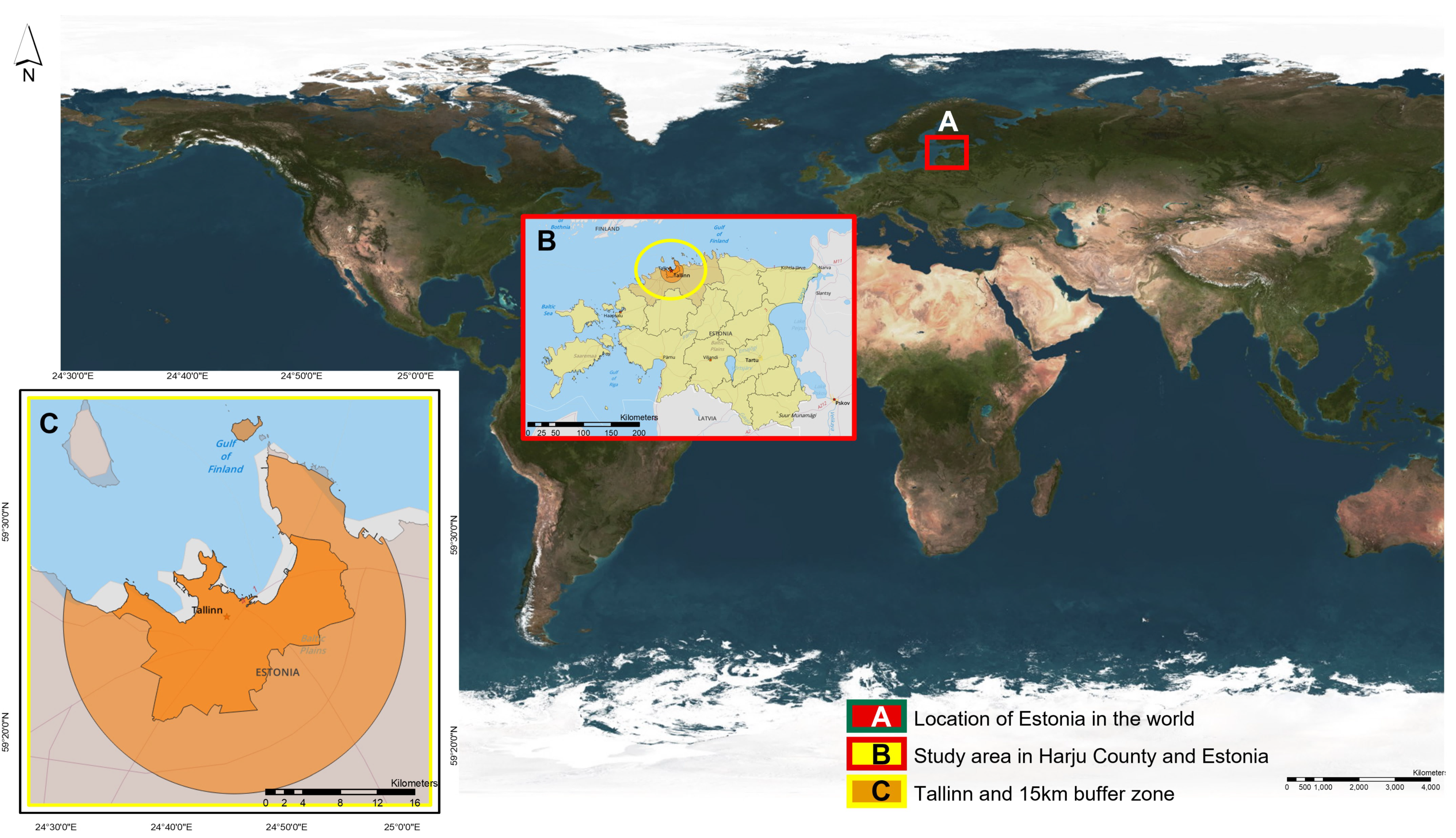
2.1. Study Area

In this paper, our focus was on built-up areas in Tallinn and its 15 km buffer zone to monitor the process of urban expansion and simulate its future trend (Figure 1). Tallinn is the capital city of Estonia and is located in the northern part of the county and neighboring the Gulf of Finland. The latitude and longitude coordinates of Tallinn region are 59.43 and 24.75. Tallinn covers a 159.37 sq. km area. Considering the 15 km buffer zone, the study area is about 506 sq. km. Essentially, the sea area in the buffer has been excluded. Between 2000 and 2017 in Estonia, 138 km2 of new built-up areas appeared, most of them around Tallinn. Mostly new dwelling areas replaced previous agricultural lands [79].
Statistics indicate that the population of Tallinn in 1990 was 479,666, which decreased by 10.19% by 2018 and reached 430,805 in total. The decrease in population has not been linear. The fastest decrease happened in the first half of the 1990s; by 2003, the population of Tallinn was 82% of that in 1990. Since 2007, a slow increase started.
Population changes in the surrounding in Harju County follow a similar pattern; the decrease from 1990 to 2000 was around 13%, increasing from then, which has brought the population back to the same level as in 1990. The dominating migration has been from Tallinn into surrounding municipalities (feeding the new settlement areas) and from other regions of Estonia to Tallinn. The particularity of the Tallinn region is that the extension of the urban area happened without significant population growth.

2.2. Data Collection

In this study, the built-up areas of 1990, 2006, and 2018 were extracted from LULC images (Table 1) resulted from the Landsat images classification using the SCP plugin in QGIS 3.10. The SCP plugin has an option to download the data from the United States Geological Survey (USGS) with radiometric and geometric corrections and the spatial record (level 1C). Using processed and georeferenced data, the projection used for this study was Lambert Conformal Conic (Estonian national grid of 1997, EPSG 3301).
The other spatial layers were road networks (main and local roads, railways), waterbodies (watercourses and lakes), and the administrative boundary of Tallinn were downloaded from the Estonian Topographic Database (ETAK) and geoportal of the land board of Estonia. Polygon data of airport and wetlands was extracted from the CORINE Landcover database. The reference year of these data was 2018 and was resampled to 30 m resolution to be consistent with the LULC data and applicable for modeling purposes.

2.3. Data Analysis

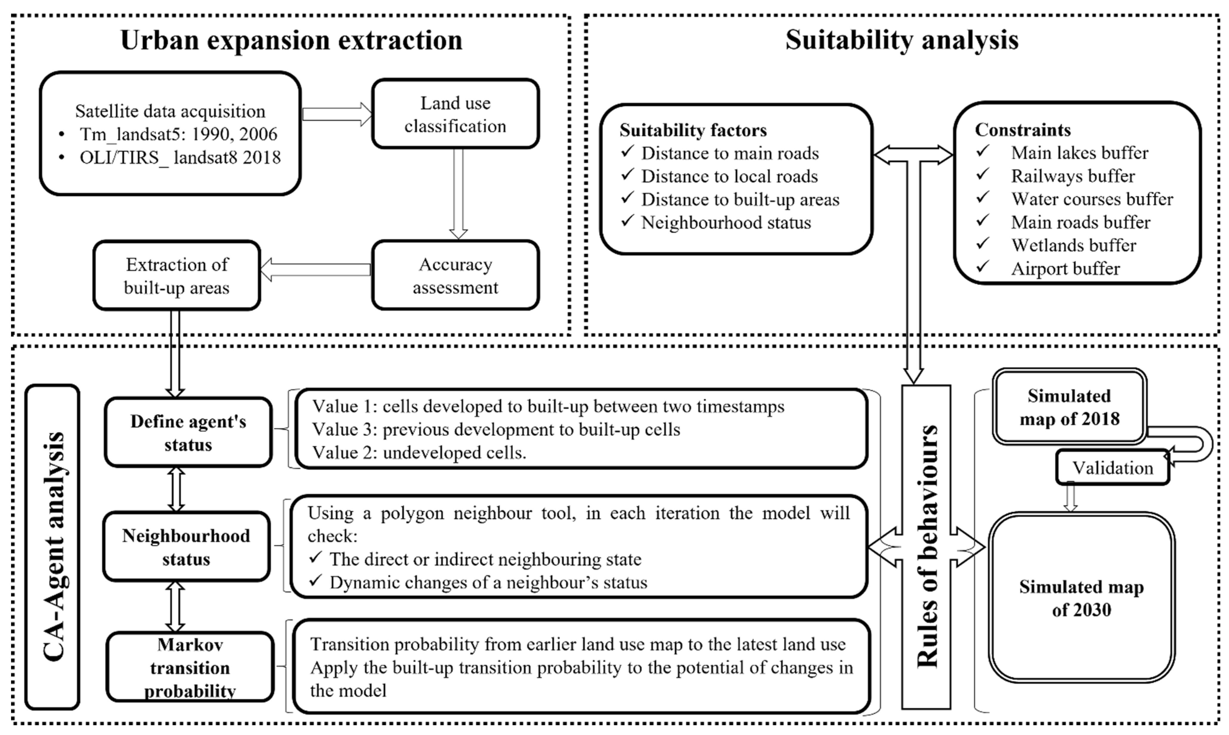
2.3.1. Image Processing

In this paper, we applied a supervised classification technique using the SCP complement for QGIS. Training samples bounded by polygons named Regions of Interest (ROIs) were obtained for four land use classes of built-up, water, vegetation, and others. Different numbers of ROIs were collected for each class. We applied the maximum likelihood (ML) classifier to obtain better results as many authors used this classifier in their research [38,80,81,82]. To assess the accuracy of maps, Google Earth [24] and the same Landsat images were used as the ground truth images. Validation of the classification was calculated based on the “Kappa coefficient”, which takes into account the agreement between observed correct and expected correct in the classified map and ground truth map [83] and “overall accuracy”, which determines the percentages of correctly classified pixels by reference pixel samples [84,85]. The Kappa coefficient mathematical expression is given as follows:
k a p p a = P 0 P e 1 P e
where P 0 indicates the observed agreement and P e is the expected agreement [63].
Overall accuracy is calculated using Equation (2):
Overall   Accuracy = 1 n K = 1 N A kk
where N is the number of classes in the LULC classification, n indicates the total number of collected sample units; Akk, which are the items in the major diagonal in the error matrix, represent the number of samples correctly identified [78].
The accuracy assessment results in Table 2 revealed excellent classification with accuracy of 98.20%, 97.80%, and 97.00% for the LULC maps of 1990, 2006, and 2018.

2.3.2. CA–Agent Model Framework

In our research, the framework’s base model is an agent-based urban growth model developed by Li [86], a scenario-based model for a city with heavy population growth. The base model was performed on the level of cadastral parcels with the ownership information in a base year and presented urban growth scenarios for 20 years. To implement our CA–Agent model, it was necessary to improve the application of the base model’s parameters, input data, procedures, and behavioral rules. To this end, the enhanced methodology and adjustment rules are defined as follows:
(a). Cellular agent: In the CA–Agent model, a discrete cell space describes an agent’s quantity or degree of development. We unified two approaches to upgrade the performance of the model. The built-up areas were dispersed in irregular polygons with different areas; however, the undeveloped cells were resized to the square polygon grids of 90 × 90 m using a fishnet tool in the GIS environment. While the processing took a long time, breaking the very large cells into smaller sizes with the fishnet tool will increase simulation results’ accuracy and cover the whole cells homogeneously. This unified vector space can provide a more realistic representation [54] of the CA–Agent model. While each cell’s status value is identical and related to the previous state, the adjacent neighboring cells and behavioral rules of the simulation model are not uniform, such that, based on different restrictions on lands, the degree of suitability of cells changes.
(b). Agent state: the state of a cellular agent is based on its temporal changes in built-up expansion. Temporal expansion of built-up areas allows investigation of agents as developed in the past or present and dedication to appropriate behavioral rules and probabilities. While the state of the agent is defined by its status and neighbors, its development status is affected by several factors such as cell size, a factor of buildable area and the least area needed for building a dwelling, the probability to be developed depending on the location of the cellular agent, whether it is in a previously developed area or an undeveloped area, also considering if it is in or near the Tallinn or suburban area, and determining the adjacent neighboring cells.
(c). Neighborhood status: the cellular agent uses the cell’s neighbor information through a list of adjacent neighbors. Using the ArcGIS polygon neighbor tool, we explored the developed and undeveloped neighbors and each cellular agent’s total number of neighbors. Table 3 represents an example of cellular agents and their adjacent neighbors after implementing the neighbor tool. The model extracts the neighbor information in each step to decide the cellular agent’s development and percentage of its change in each time step to see if a neighbor has direct or indirect neighboring state as well as accessibility to local roads, which could be a grant for a cell to be accessed through its neighbors. Therefore, the dynamic changes of a neighbor’s status is a factor in a cell’s suitability. The neighboring cells influence the cells’ development status within defined information, updated in each step. To delineate the heterogeneity of neighborhood effects, we defined the adjacent neighbors implemented in the base model [86] instead of using the Moore neighborhood, which is the most frequently used neighborhood [54] or applying a specified distance neighbor, which depends on the distance of neighbors from a kernel cell [44].
(d). Markovian transition probability: Adding a probability and randomness to the agent’s behavior is critical in the simulation [64]. In the base model, the probability was determined in a random term. In contrast, the Markovian transition probability in the CA–Agent model was performed to add complexity to the agent’s behavior and calculate the transition probability in built-up for two time periods from 1990 to 2006 and 2006 to 2018.
(e). Suitability factors and constraints: Analysis of suitability, which acts as environmental rules, was carried out using different accessibility factors that shape a cellular agent’s behavior’s suitability decision considering the dynamics of the study area’s environment, neighborhood, and spatial characteristics. Constraints mainly refer to the factors preventing expansion [87]. The distance analysis was based on the Euclidean distance tool, and the constraints were analyzed using the buffer tool and fuzzy overlay analysis in the GIS environment. Like the base model with different selected suitability factors and constraints, in the CA–Agent model, the constraints are permanent during the run process and are precalculated to extract the number of unbuildable cells ahead of time. The ranges of suitability factors are between 0 and 100. During the model run, cellular agents normalized suitability rates to reach the actual value for each factor. The constraints and factors were converted to raster, and all the operations of cells run in the raster environment.
(f). Thresholds role in the agent’s development status: Expansion of a city may face different physical limitations known as development thresholds [87]. Defining a threshold for the factors is necessary to give the complexity and reality to an agent’s model and development status and boost the spatial heterogeneity. The CA–Agent model employs the exact terminology of allocating the thresholds to the agents. Thresholds are calculated based on the integration of constraints and factors during the initialization of the model.
(g). Behavioral rules: The behavioral rules form the development status of agents. These rules depend on different factors: the status of a cell, its neighbors, suitability criteria, constraints, and accessibility factors. Among other things, “if the cellular agent’s ratio of unbuildable area to total area exceeds the threshold, then the agent will not be developed”; “if it falls in a constraint area, then it exhibited change”; and “if more neighbors are built up, then it is likely to develop” are the most critical behavioral rules. Consequently, the CA–Agent model can consider many rules that reflect the actual urban expansion process over time and space. Therefore, the number of cells changing their states is entirely defined by behavioral rules.
Two-time steps of 12 years were used in this research for two simulated maps of 2018 and 2030. In the first simulation, the model run 12-time steps representing years between 2006 and 2018, resulting in the simulated map of 2018. After performing the validation, we executed the second model run resulting in the simulated urban expansion map of 2030.
Figure 2 is a flowchart representing the methods for spatial data analysis and CA–Agent analysis; a process is performed in this paper.

3. Results

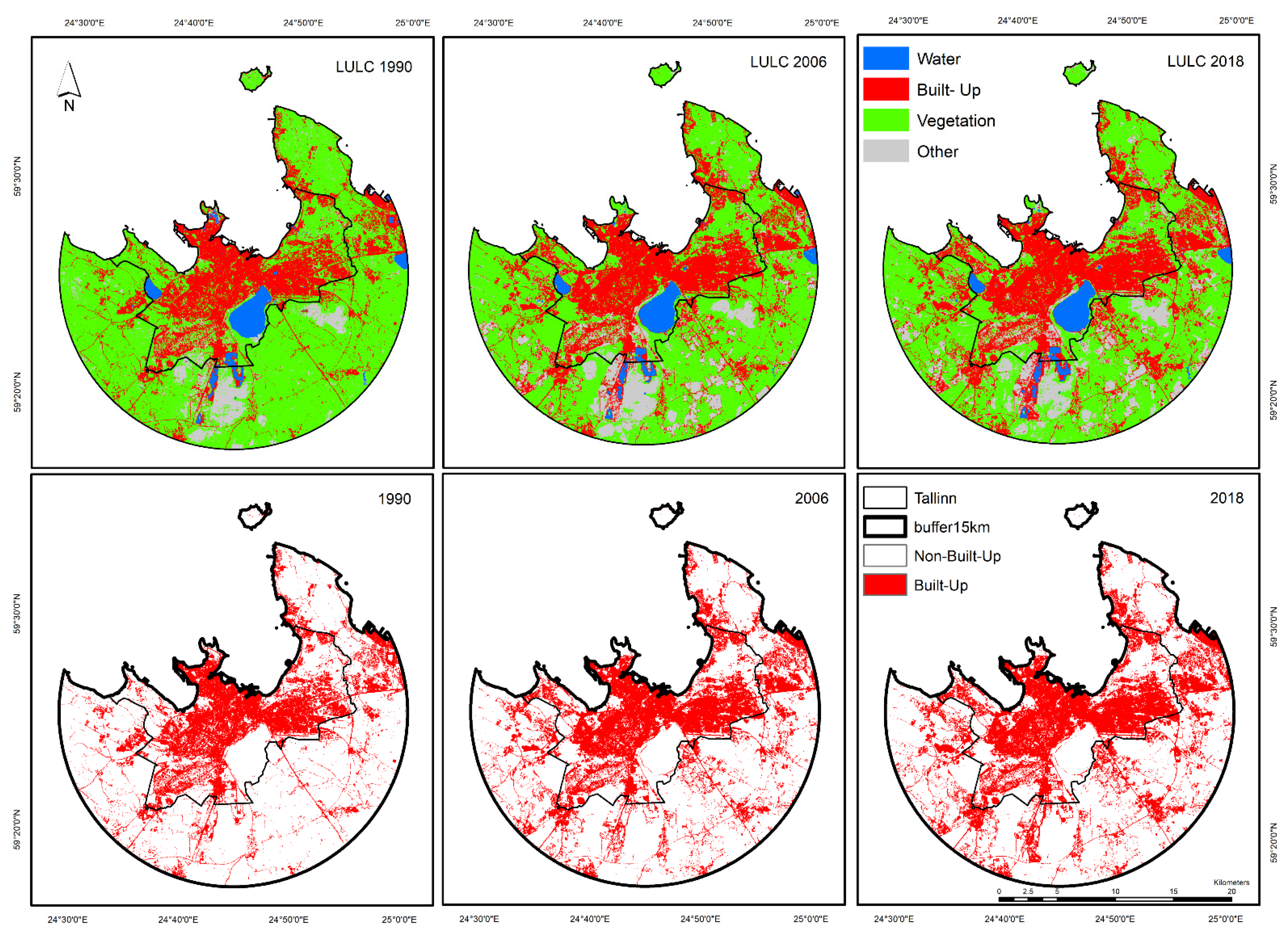
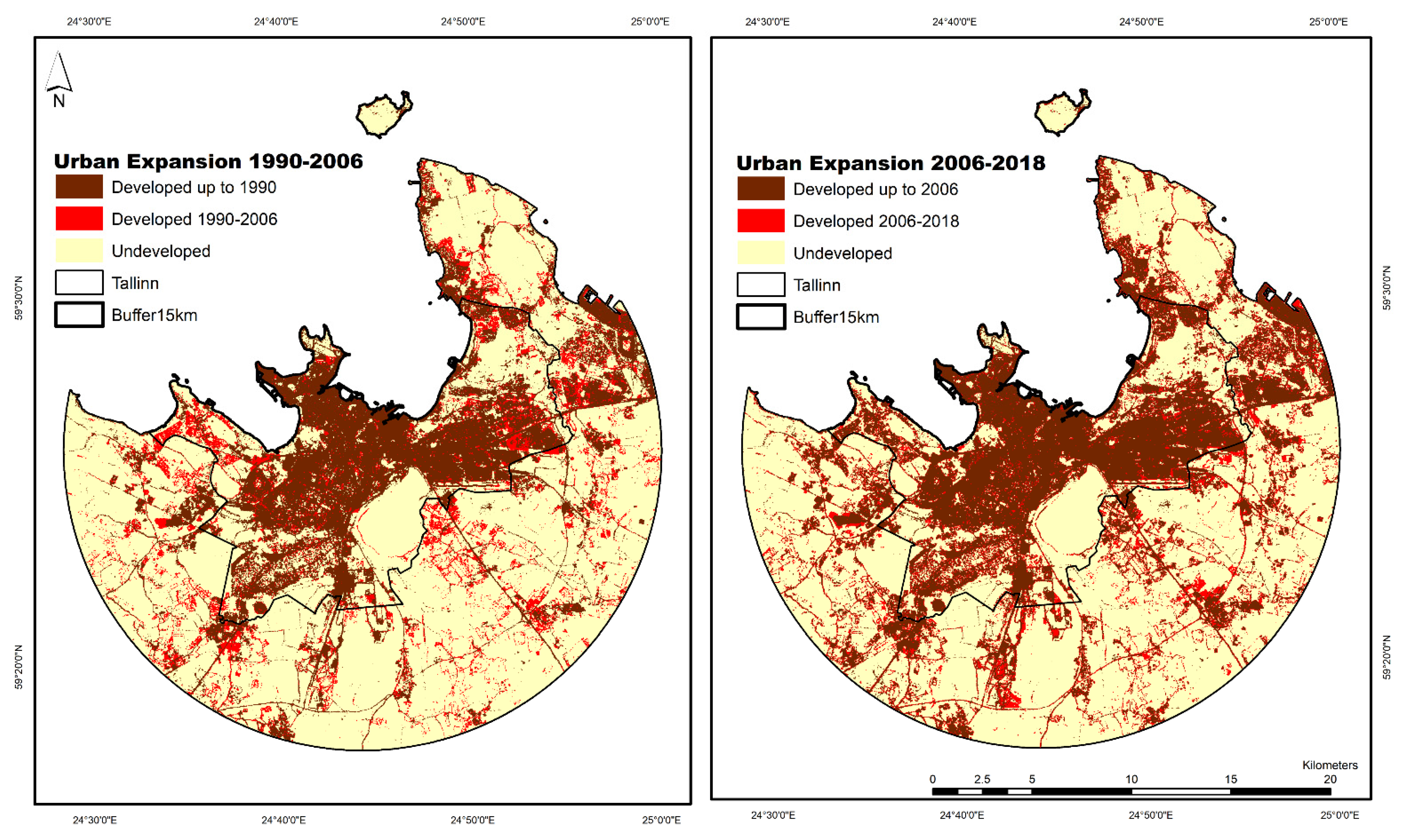
3.1. Spatiotemporal Patterns of Urban Expansion from 1990 to 2018

According to the LULC classification in this study, we adopted four classes: water (including rivers, ponds, and lakes), built-up (consisting of residential, industrial, and other impervious surfaces), vegetation (including evergreen forest, agriculture, and areas mostly of grass), and other (covering bare earth, rocks, and wetland areas). As shown in Figure 3, changes are represented for three years of 1990, 2006, and 2018. To visualize the urban expansion and its distribution, the built-up areas were extracted in the GIS environment for the mentioned years.
As shown in Table 4, urban areas during the 28 years increased by 40.80 sq. km (+25.03% change) in Tallinn and its 15 km buffer zone. Urban expansion during 1990–2006 was 27.10 sq. km (18.15% increase), faster than the expansion of urban areas between 2006 and 2018, which was 13.70 sq. km and a rise of 8.40% in this timestamp.

3.2. Application of CA–Agent Model in Tallinn and Its Buffer Zone

In our model, an irregular polygon stated a cell. The cells are the dynamic agents. As shown in Figure 4, cellular agents have three different values; Value 1 is allocated to the cells developed to be built up between two timestamps, Value 3 is the previous development to be built up, and Value 2 shows the undeveloped cells. It is an irregular spatial unit that provides the situation closer to reality. The cell’s size in the undeveloped area with Value 2 ranges from 127 to 8100 sq. m, while the agents with Value 3 are defined to show the initial development of Tallinn and surroundings; during the model run, Value 2 agents have less likelihood to be developed in the neighboring areas unless they have high probability of being located in Tallinn or being a large cell. Neighboring with Value 1 agents who developed later than Value 3, the probability of being large, isolated, in Tallinn, or the buffer zone will be evaluated.
We took advantage of Markovian transition probability results to allocate the probabilities in our model, which is presented in many factors such as the probability of a cellular agent to be developed depending on its size and its location if it is in a previously developed area, within the built-up area or suburban (Table 5).
Additionally, suitability factors consist of “distance to Tallinn”, “distance to main roads”, “distance to local roads”, and “neighborhood status”. Six constraints were defined to limit the buildable lands, which was a fuzzy overlay combination of “50 m buffer of main lakes”, “30 m buffer of railways”, “25 m buffer zone of watercourses”, “50 m buffer of main roads”, “50 m buffer of the airport”, and “50 m buffer of wetlands”. The constraints, regardless of their land LULC classes, play leading roles in determining the buildability of the agents. We applied different restrictions on constraints based on the guidelines of Estonian legislation on new constructions named “Riigi Teataja”. This building code was prepared to promote sustainable development and ensure constructions’ safety and purposeful performance in Estonia. It has differentiated the construction restrictions upon the type of the protected zones, whether roads, railways, water, or other zones. Figure 5 represents the results of indices analysis.

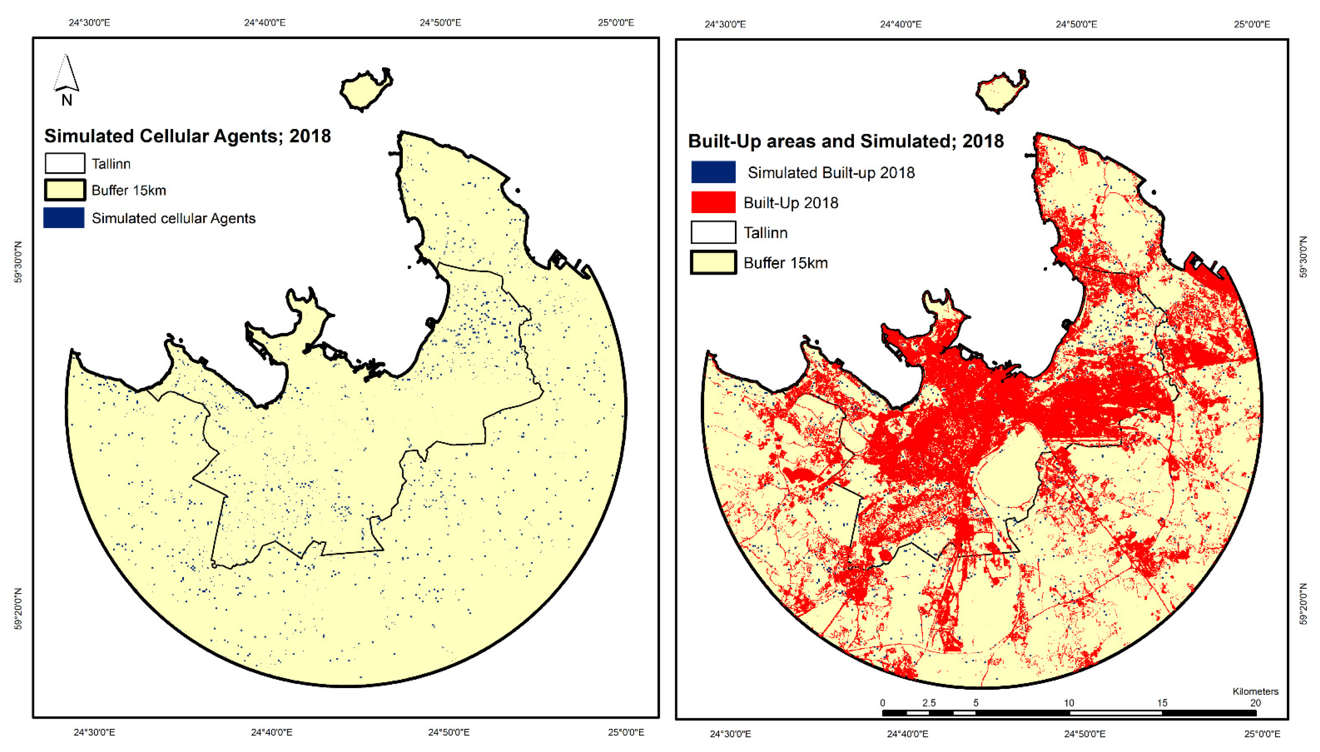
3.3. Simulation of Urban Expansion by 2018

In this step, each cell has one value. Based on the built-up states, if a cell is developed before 1990, its value is assumed to be 3. If a cell is developed between 1990 and 2006, its value is 1, and if it is undeveloped, its status value is 2. The cellular agent can change its status in each time step. At each iteration, the agent re-evaluates its current conditions based on the several probabilities of changes and behavioral rules and decides whether to change them or not. The simulated map of urban expansion for 2018 is represented in Figure 6.
Table 6 illustrates the results of the statistics of the model run. From the total of 73,815 cells, 54,707 were undeveloped cells with a state of 2. Considering the cells’ size, cellular agents’ spatial location, adjacent neighborhood, the suitability factors, and probability of transition, 1770 cells determined unbuildable cells. The model verified the sum of the suitable land and reached the threshold of 88%. After the 12 runs of the model’s total number of developed cells reached 20,844, cells increased by 1736 cells during the 12-year simulation. The total area of built-up added in this time was 7.06 square kilometers.

3.4. Simulation Validation Results

The first two built-up maps of 1990 and 2006 were used to validate the simulation model. Validation aims to explore how actual data fits the model output [82,88]. Using the Validate option in IDRISI, its statistical analysis results in the quantity of cells agreement/disagreement and the agreement/disagreement in cells location.
The first simulation for the year 2018 on built-up areas was validated against the actual map of built-up areas in 2018. Table 7 indicates the statistical results of the validation. “Kstandard” is the Kappa coefficient, “Klocation” refers to the kappa for the grid-cell level location to monitor how well the grid cells are located on the landscape, “MediumGrid (m)” calculates the agreement between the reference map of 2018 and the simulation map in terms of proportion correct [89], “Qdisagreement”, proposed by Pontius and Millones [90] as an alternative to Kappa, determines the amount of disagreement regarding the fails in specifying the correct quantity of each category of comparison map with the reference map, and Adisagreement counts error in match the spatial allocations due to differences in the location of comparison and the reference map categories [89,90,91].
Kappa’s result denotes that the higher the index value, the better the accuracy, while Kappa > 0.8 indicated very high accuracy [34]. From the results of the image comparison between the simulated map of 2018 and the LULC map, it was evident that Kstandard (0.86), Klocation (0.89), and MediumGrid (m) (0.91) demonstrated high accuracy of the simulated map, while the Qdisagreement (0.02) and Adisagreement (0.07) declared minor cell error match in the simulation result. Therefore, it is clear that CA–Agent model runs reached an acceptable prediction, and it can be concluded that the simulated parameters fit the reality.

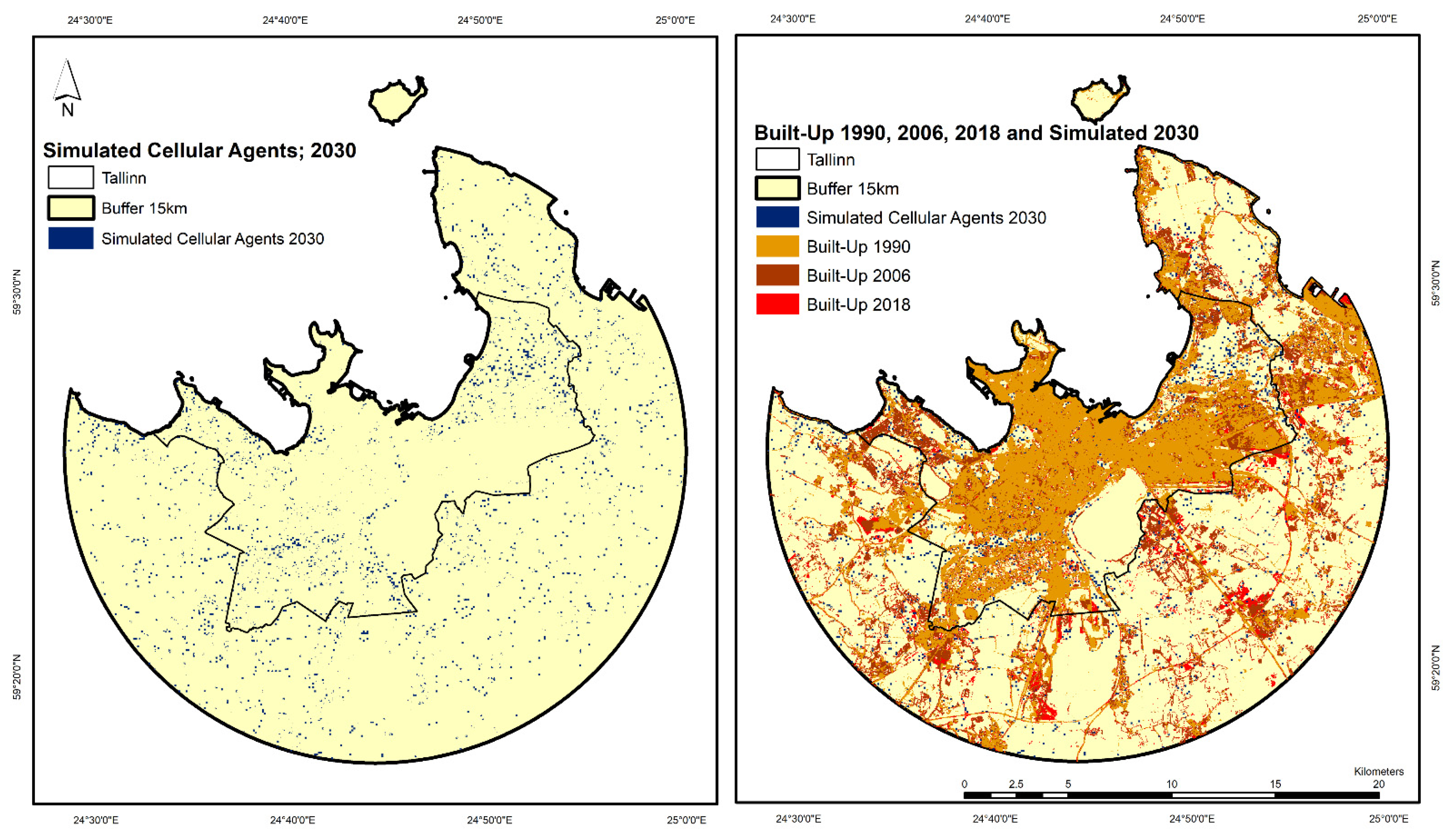
3.5. Simulation of Urban Expansion by 2030

Employing comparative analysis, the CA–Agent model’s result provides evidence of the close resemblance with the actual data of built-up. Therefore, simulation of the built-up area for 2030 can be experimented with by applying this algorithm. Therefore, we performed the second run of 12-time steps for simulating the urban expansion by 2030; the simulated results are shown in Figure 7.
Table 8 illustrates the results of the statistics of the model run. It is evident from the table that, from the total of 69,624 cells, 58,236 were undeveloped cells. A total of 2342 cells were determined to be unbuildable cells, and the threshold of the suitable lands reached 94%. After the 12 runs of the model, the total number of 2881 cells were developed, with the total areas of 12.22 square kilometers adding to built-up areas. The simulation results revealed that the built-up areas would expand by 6.97% from 2018 to 2030.

4. Discussion

The complexity of simulation of the urban expansion in cities and suburbs needs decision making about the proper factors affecting the phenomena. While it is not adequate to observe the simulation over one model [92], hybrid modeling leads to better results. Coupling the cellular automata, Markov, and agent-based modeling in a GIS environment in this study led to a simulation of the urban expansion in Tallinn and its buffer zone. It is worth discussing the implemented components of the CA–Agent model demonstrated in this paper as follows:

4.1. Interactions of Cellular Agents

Integrating the cellular automata and agent-based models in our research allowed us to synthesize the probabilities and rules into one model. This capability allowed the cellular agents to decide the probability of spatial transition and the rules of behavior on interacting with the other cellular agents and their environment. In line with Wahyudi et al. [72], we applied interactions between “cellular agents to cellular agents” through making a query and extracting information from other cellular agents and “cellular agents to the environment” through influencing it by modifying the cell status from non-urban to urban. In other words, we have defined the interactions in several steps. First, a cellular agent searched the lands and collected the information for the probable development status depending on the cell’s size, the least area needed for building a dwelling, the location, and adjacent neighboring cells. Then, it assessed the situation based on the behavioral rules, suitability, and probability of developing it. Reaching the thresholds allowed the cellular agent to take the development action, where constraints and limitations of transition defined the cellular agents’ response to be developed during the model run. Thus, the most crucial step in the model was defining cellular agents’ interactions to reach the development decision.

4.2. Applying the Adjacent Neighborhood

We have verified that the neighbor’s status is an initial element of behavioral rules and a prerequisite for a cellular agent’s development action. Research on neighborhood effects mostly applied a kernel cell influenced by its neighbors such as a Moore neighborhood [93,94] or a distance decay neighborhood [44]. We did not replicate the previous research; instead, we applied the adjacent cell’s neighborhood considering the polygon neighbor list, which could cover all the possibilities of the accessibility by neighbors. The adjacent neighborhood is based on the spatial and quantity influence of neighbors [95]. It can implicitly address spatial heterogeneity; through the adjacent polygon neighbor list, the cellular agent assessed the number and proportion of neighbors that have developed at each time step and made its development decision. If no immediate neighbor or neighbor’s neighbor has been developed, the cellular agent’s probability value to develop was small.

4.3. State of the Cellular Agent

Typically, many studies have employed a lattice of square cells or a raster data surface as the state of their agents [72,94,96]. In contrast, some other researchers tried to develop irregular space states for their simulations [73,97]. Regular cells rarely represent the basic unit of land use, so adopting a conventional regular cell-based CA model could affect the performance of the simulation. Instead, applying an irregular structure of cells with different sizes can better represent the reality [98] of urban expansion, which took place in a non-uniform space. Therefore, in our model, we have integrated the regular environment and irregular cells in the data model and operations, which performed more realistically in capturing the geometric details. We showed that the cellular agent’s development status depends on different factors such as accessibility and suitability. Therefore, a cellular agent’s final state changed to built-up when a cell passed the whole assessment tests. It is consistent with what has been found in the research by Dahal and Chow [73] on the level of irregular cadastral land parcels, Pinto and Antunes [99] on the level of irregular cells of census blocks, and Chen et al. [98] on the level of patch-based simulation.

4.4. Coupling Markovian Transition Probability with CA–Agent

Using Markov Model integrated with cellular automata is a widely used technique to describe the likelihood of the state for conversion between two timestamps. It estimates the transition probability [38,100,101,102] as the potential changes of the future. Berberoğlu et al. [103] have shown that conditional probabilities of the Markov model are reliable for allocating the to-be-changed state of cells. A similar application of the Markov model was obtained by Aburas et al. [68] in predicting the quantity of urban and non-urban areas. However, in line with the idea of Xu et al. [69], we agreed that to overcome the limitations of the Markov model, it is required to integrate results with other models. In this case, investigating the values of transition probability of Markov in a CA–Agent model is a new approach that we employed in our model. Instead of randomly assigning the probability values to the change factors, we used Markovian transition probability, which extracted the spatial conversion during the time, resulting in a better projection of agent cell development status.

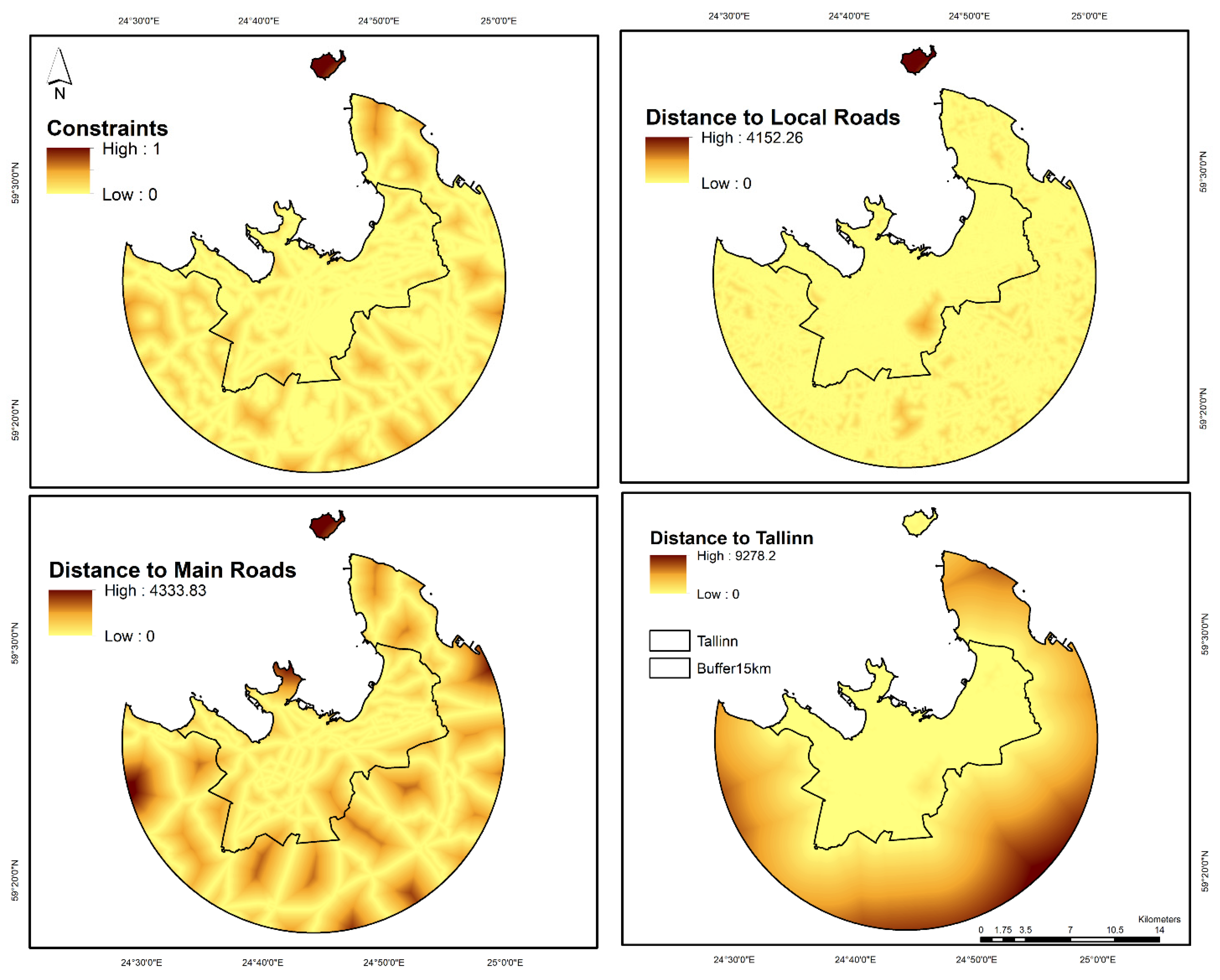
4.5. Configuration of Suitability Factors

Suitability factors play essential roles in the model configuration, indicating the state of the agent’s likelihood to develop from a non-developed to a developed one. In our model, the cellular agents made their decision regarding the influence of some factors consist of “distance to Tallinn”, “distance to main roads”, “distance to local roads”, and “neighborhood status”. The different variables mainly depend on the reality of driving forces of urban expansion in the study area and changes regarding modifying the extent. In line with the study performed by Mozaffaree Pour and Oja. [47] on the same area, we reached the selected factors. Additionally, Tan et al. [93] demonstrated that distance to the city center, major roads, and the main river negatively influences urban expansion. Similarly, Mustafa et al. [50] used the distance factors to roads, towns, and railways, and Liu et al. [94] applied spatial variables of distance to the town center, roads, and water as the suitability factor.

4.6. Urban Expansion Simulation

During the 28 years from 1990 to 2018, built-up areas increased by 25.03% in Tallinn and its 15 km buffer zone. The increase of urban areas despite the decrease in population characterizes changes in the way of life. Urban expansion during 1990–2006 had risen by 18.15%, which was faster than the expansion of urban areas between 2006 and 2018 with an 8.40% increase. We performed the model run two times, in 2018 and 2030. The first 12-years runs represented 1736 cells converting from undeveloped status to developed. Then, we evaluated the performance of the model by operating the Kappa Index of Agreement. It shows a degree of 0.86, a relatively high degree of correct simulation result for the first simulated map. Similar trends have been observed in actual data in the research by Oja [79] in Estonia.
Further, we performed the second simulation for the year 2030. After the 12 runs of the model, 2881 cells were developed, with 12.22 square kilometers adding to built-up areas. Therefore, the total built-up areas from 1990 to 2030 will reach 175.24 sq. km with an increase of 30.25% in total. The result is in good accordance with the actual changes.

4.7. Research Limitations

Besides many advantages of the CA–Agent model in simulating the cellular agents’ interactions over time, this research has some limitations. Because of the lack of time-series spatial data in the cadastral level in the study area, we decided to investigate the model at the cell level. While implementing the CA–Agent model with precise spatiotemporal cadastral data will generate simulation closer to reality, another limitation involves the inherent of the model itself, as each model has its limitation. The CA–Agent model, like the other simulation models, suffers from the extrapolation of past trends. It is a constraints-driven model rather than a preference-led model and lacks the dimension of human decision. Furthermore, despite significant advancement in computing and modeling, there is still the issue of complexity in urban systems, which requires mediating knowledge with the reality of environmental changes.

5. Conclusions

Trade-offs between agriculture, forest, and built-up lands need simulation modeling approaches to link expansion orientation and quantify spatial planning activities. In this paper, we employed the CA–Agent model to monitor the process of urban expansion and simulate urban expansion in Tallinn and its 15 km buffer zone. Application of the CA–Agent model for spatial planning activities let us consider how implementing different driving factors, probability of changes, and modifying thresholds will affect the outputs of the model and the distribution of the built-up over time. Correspondingly, spatially explicit consequences of urban expansion support the effective decision making across the cellular agent’s characteristics and rules of behavior in spatial planning.
It is essential to highlight that even though the built-up area in the study area increased by 25.03%, the population of Tallinn decreased by 10.19% between 1990 and 2018. The dominating migration has been from Tallinn into surrounding municipalities (feeding the new settlement areas) and from other regions of Estonia to Tallinn.
In this regard, modeling the factors affecting urban expansion in Tallinn area is critical to detect future expansion trends. The integrated CA–agent model in our research allowed us to synthesize the probabilities and enhance the rules into one model. This capability allowed the cellular agents to decide the probability of spatial transition and the rules of behavior on interacting with the other cellular agents and their environment. The main conclusion that can be notified is that taking advantage of cellular-based modeling, adjacent neighborhood information, and Markovian transition probability provides the simulated map of urban expansion in 2018 with a Kappa degree of 0.86, which confirms a relatively high accuracy of the implemented model components. Consequently, the model was considered “approved” for simulating the urban expansion in 2030. Thus, implementing the CA–Agent model in the study area illustrated the temporal changes of land conversion and represented the present spatial planning results requiring regulation of urban expansion encroachment on agricultural and forest lands.
This conclusion follows that urban expansion is a dynamic spatial process affected by different physical drivers. We considered the suitability factors of “distance to Tallinn”, “distance to main roads”, “distance to local roads” and “neighborhood status” and six constraints, namely, “main lakes”, “railways”, “watercourses”, “main roads”, “airport”, and “wetlands”. It best suits the simulation results to consider the social and economic factors that could be conducted in future studies. Altogether, the modeling proves urban expansion as a result of unplanned sprawl.

Author Contributions

N.M.P.: conceptualization, methodology, formal analysis, writing—original draft, and visualization; T.O.: supervision, conceptualization, resources, writing—review and editing, and project administration. All authors have read and agreed to the published version of the manuscript.

Funding

The Estonian Research Council grant PRG352 has supported the research.

Institutional Review Board Statement

Not applicable.

Informed Consent Statement

Not applicable.

Data Availability Statement

Not applicable.

Acknowledgments

The authors thank Luca Congedo, author/developer of the Semi-Automatic Classification Plugin for QGIS, which guided the process of classification of LULC maps. Special thanks to the academic editor and three anonymous reviewers for their constructive suggestions that significantly strengthened this manuscript.

Conflicts of Interest

The authors declare no conflict of interest.

References

  1. He, C.; Liu, Z.; Gou, S.; Zhang, Q.; Zhang, J.; Xu, L. Detecting Global Urban Expansion over the Last Three Decades Using a Fully Convolutional Network. Environ. Res. Lett. 2019, 14, 034008. [Google Scholar] [CrossRef]
  2. Haregeweyn, N.; Fikadu, G.; Tsunekawa, A.; Tsubo, M.; Meshesha, D.T. The Dynamics of Urban Expansion and Its Impacts on Land Use/Land Cover Change and Small-Scale Farmers Living near the Urban Fringe: A Case Study of Bahir Dar, Ethiopia. Landsc. Urban Plan. 2012, 106, 149–157. [Google Scholar] [CrossRef]
  3. Forkuor, G.; Cofie, O. Dynamics of Land-Use and Land-Cover Change in Freetown, Sierra Leone and Its Effects on Urban and Peri-Urban Agriculture—A Remote Sensing Approach. Int. J. Remote Sens. 2011, 32, 1017–1037. [Google Scholar] [CrossRef]
  4. Bolca, M.; Turkyilmaz, B.; Kurucu, Y.; Altinbas, U.; Esetlili, M.T.; Gulgun, B. Determination of Impact of Urbanization on Agricultural Land and Wetland Land Use in Balçovas’ Delta by Remote Sensing and GIS Technique. Environ. Monit. Assess. 2007, 131, 409–419. [Google Scholar] [CrossRef] [PubMed]
  5. Salghuna, N.N.; Rama Chandra Prasad, P.; Asha Kumari, J. Assessing the Impact of Land Use and Land Cover Changes on the Remnant Patches of Kondapalli Reserve Forest of the Eastern Ghats, Andhra Pradesh, India. Egypt. J. Remote Sens. Space Sci. 2018, 21, 419–429. [Google Scholar] [CrossRef]
  6. Bala, G.; Caldeira, K.; Wickett, M.; Phillips, T.J.; Lobell, D.B.; Delire, C.; Mirin, A. Combined Climate and Carbon-Cycle Effects of Large-Scale Deforestation. Proc. Natl. Acad. Sci. USA. 2007, 104, 6550–6555. [Google Scholar] [CrossRef] [Green Version]
  7. Huang, J.; Zhan, J.; Yan, H.; Wu, F.; Deng, X. Evaluation of the Impacts of Land Use on Water Quality: A Case Study in the Chaohu Lake Basin. Sci. World J. 2013, 2013. [Google Scholar] [CrossRef] [PubMed] [Green Version]
  8. McGrane, S.J. Impacts of Urbanisation on Hydrological and Water Quality Dynamics, and Urban Water Management: A Review. Hydrol. Sci. J. 2016, 61, 2295–2311. [Google Scholar] [CrossRef]
  9. Patra, S.; Sahoo, S.; Mishra, P.; Mahapatra, S.C. Impacts of Urbanization on Land Use /Cover Changes and Its Probable Implications on Local Climate and Groundwater Level. J. Urban Manag. 2018, 7, 70–84. [Google Scholar] [CrossRef]
  10. Bhat, P.A.; ul Shafiq, M.; Mir, A.A.; Ahmed, P. Urban Sprawl and Its Impact on Landuse/Land Cover Dynamics of Dehradun City, India. Int. J. Sustain. Built Environ. 2017, 6, 513–521. [Google Scholar] [CrossRef]
  11. Li, C.; Zhao, J.; Thinh, N.X.; Xi, Y. Assessment of the Effects of Urban Expansion on Terrestrial Carbon Storage: A Case Study in Xuzhou City, China. Sustainability 2018, 10, 647. [Google Scholar] [CrossRef] [Green Version]
  12. Zubair, O.A.; Ji, W.; Weilert, T.E. Modeling the Impact of Urban Landscape Change on Urban Wetlands Using Similarityweighted Instance-Based Machine Learning and Markov Model. Sustainability. 2017, 9, 2223. [Google Scholar] [CrossRef] [Green Version]
  13. Kelobonye, K.; Xia, J.C.; Swapan, M.S.H.; McCarney, G.; Zhou, H. Drivers of Change in Urban Growth Patterns: A Transport Perspective from Perth, Western Australia. Urban Sci. 2019, 3, 40. [Google Scholar] [CrossRef] [Green Version]
  14. Qian, Y.; Wu, Z. Study on Urban Expansion Using the Spatial and Temporal Dynamic Changes in the Impervious Surface in Nanjing. Sustainability 2019, 11, 933. [Google Scholar] [CrossRef] [Green Version]
  15. Mohapatra, S.N.; Pani, P.; Sharma, M. Rapid Urban Expansion and Its Implications on Geomorphology: A Remote Sensing and GIS Based Study. Geogr. J. 2014, 2014. [Google Scholar] [CrossRef] [Green Version]
  16. D’Amour, C.B.; Reitsma, F.; Baiocchi, G.; Barthel, S.; Güneralp, B.; Erb, K.H.; Haberl, H.; Creutzig, F.; Seto, K.C. Future Urban Land Expansion and Implications for Global Croplands. Proc. Natl. Acad. Sci. USA 2017, 114, 8939–8944. [Google Scholar] [CrossRef] [Green Version]
  17. Castle, C.J.E.; Crooks, A. Principles and Concepts of Agent-Based Modelling for Developing Geospatial Simulations. Available online: https://discovery.ucl.ac.uk/id/eprint/3342/1/3342.pdf (accessed on 1 September 2006).
  18. Wang, J.; Gao, W.; Gao, Z.; Yin, J.; Xu, S. Urban Expansion and Landscape Diversity Change of Shanghai City. Available online: https://www.researchgate.net/publication/252987453_Urban_Expansion_and_Landscape_Diversity_Change_of_Shanghai_City_China (accessed on 12 August 2010).
  19. Dahal, K.R.; Benner, S.; Lindquist, E. Analyzing Spatiotemporal Patterns of Urbanization in Treasure Valley, Idaho, USA. Appl. Spat. Anal. Policy 2016, 11, 205–226. [Google Scholar] [CrossRef]
  20. Van Truong, T.; Van Cu, P.; Laffly, D. Urban Expansion and Landscape Change Analysis Using Remote Sensing and Survey: A Case Study in Ha Long Bay Area, Vietnam. In Proceedings of the IEEE 2016 Eighth International Conference on Knowledge and Systems Engineering (KSE), Hanoi, Vietnam, 6–8 October 2016; pp. 315–320. [Google Scholar] [CrossRef]
  21. Zhao, P.; Lü, B.; de Roo, G. Urban Expansion and Transportation: The Impact of Urban Form on Commuting Patterns on the City Fringe of Beijing. Environ. Plan. Econ. Space 2010, 42, 2467–2486. [Google Scholar] [CrossRef]
  22. Zhao, P. Sustainable Urban Expansion and Transportation in a Growing Megacity: Consequences of Urban Sprawl for Mobility on the Urban Fringe of Beijing. Habitat Int. 2010, 34, 236–243. [Google Scholar] [CrossRef]
  23. Rimal, B.; Zhang, L.; Keshtkar, H.; Haack, B.N.; Rijal, S.; Zhang, P. Land Use/Land Cover Dynamics and Modeling of Urban Land Expansion by the Integration of Cellular Automata and Markov Chain. ISPRS Int. J. Geo-Inf. 2018, 7, 154. [Google Scholar] [CrossRef] [Green Version]
  24. Xu, S.; Sun, Y.; Zhao, S. Contemporary Urban Expansion in the First Fastest Growing Metropolitan Region of China: A Multicity Study in the Pearl River Delta Urban Agglomeration from 1980 to 2015. Urban Sci. 2021, 5, 11. [Google Scholar] [CrossRef]
  25. Deep, S.; Saklani, A. Urban Sprawl Modeling Using Cellular Automata. Egypt. J. Remote Sens. Space Sci. 2014, 17, 179–187. [Google Scholar] [CrossRef] [Green Version]
  26. Wang, R.; Hou, H.; Murayama, Y. Scenario-Based Simulation of Tianjin City Using a Cellular Automata-Markov Model. Sustainability 2018, 10, 2633. [Google Scholar] [CrossRef] [Green Version]
  27. Chen, G.; Li, X.; Liu, X.; Chen, Y.; Liang, X.; Leng, J.; Xu, X.; Liao, W.; Qiu, Y.; Wu, Q.; et al. Global Projections of Future Urban Land Expansion under Shared Socioeconomic Pathways. Nat. Commun. 2020, 11, 1–12. [Google Scholar] [CrossRef] [Green Version]
  28. Harb, M.; Garschagen, M.; Cotti, D.; Krätzschmar, E.; Baccouche, H.; Ben Khaled, K.; Bellert, F.; Chebil, B.; Ben Fredj, A.; Ayed, S.; et al. Integrating Data-Driven and Participatory Modeling to Simulate Future Urban Growth Scenarios: Findings from Monastir, Tunisia. Urban Sci. 2020, 4, 10. [Google Scholar] [CrossRef] [Green Version]
  29. Mustafa, A.; Cools, M.; Saadi, I.; Teller, J. Coupling Agent-Based, Cellular Automata and Logistic Regression into a Hybrid Urban Expansion Model (HUEM). Land Use Policy 2017, 69, 529–540. [Google Scholar] [CrossRef] [Green Version]
  30. Falah, N.; Karimi, A.; Tavakoli Harandi, A. Urban Growth Modeling Using Cellular Automata Model and AHP (Case Study: Qazvin City). Model. Earth Syst. Environ. 2020, 6, 235–248. [Google Scholar] [CrossRef] [Green Version]
  31. Benchelha, M.; Benzha, F.; Rhinane, H.; Benchelha, S.; Benchelha, T. Modeling of Urban Growth Using Cellular Automata and GIS Case of Benslimane in Morocco. Available online: https://doi.org/10.20944/preprints202011.0287.v1 (accessed on 9 November 2020).
  32. Liu, Y.; Batty, M.; Wang, S.; Corcoran, J. Modelling Urban Change with Cellular Automata: Contemporary Issues and Future Research Directions. Prog. Hum. Geogr. 2021, 45, 3–24. [Google Scholar] [CrossRef]
  33. Guan, D.; Zhao, Z.; Tan, J. Dynamic Simulation of Land Use Change Based on Logistic-CA-Markov and WLC-CA-Markov Models: A Case Study in Three Gorges Reservoir Area of Chongqing, China. Environ. Sci. Pollut. Res. 2019, 26, 20669–20688. [Google Scholar] [CrossRef] [PubMed]
  34. Li, X.; Wang, M.; Liu, X.; Chen, Z.; Wei, X.; Che, W. MCR-Modified CA-Markov Model for the Simulation of Urban Expansion. Sustainability 2018, 10, 3116. [Google Scholar] [CrossRef] [Green Version]
  35. Guan, D.J.; Li, H.F.; Inohae, T.; Su, W.; Nagaie, T.; Hokao, K. Modeling Urban Land Use Change by the Integration of Cellular Automaton and Markov Model. Ecol. Model. 2011, 222, 3761–3772. [Google Scholar] [CrossRef]
  36. Sarkar, A.; Chouhan, P. Modeling Spatial Determinants of Urban Expansion of Siliguri a Metropolitan City of India Using Logistic Regression. Model. Earth Syst. Environ. 2020, 6, 2317–2331. [Google Scholar] [CrossRef]
  37. Salem, M.; Tsurusaki, N.; Divigalpitiya, P. Analyzing the Driving Factors Causing Urban Expansion in the Peri-Urban Areas Using Logistic Regression: A Case Study of the Greater Cairo Region. Infrastructures 2019, 4, 4. [Google Scholar] [CrossRef] [Green Version]
  38. Siddiqui, A.; Siddiqui, A.; Maithani, S.; Jha, A.K.; Kumar, P.; Srivastav, S.K. Urban Growth Dynamics of an Indian Metropolitan Using CA Markov and Logistic Regression. Egypt. J. Remote Sens. Space Sci. 2018, 21, 229–236. [Google Scholar] [CrossRef]
  39. Koch, J.; Dorning, M.A.; Van Berkel, D.B.; Beck, S.M.; Sanchez, G.M.; Shashidharan, A.; Smart, L.S.; Zhang, Q.; Smith, J.W.; Meentemeyer, R.K. Modeling Landowner Interactions and Development Patterns at the Urban Fringe. Landsc. Urban Plan. 2019, 182, 101–113. [Google Scholar] [CrossRef]
  40. Hosseinali, F.; Alesheikh, A.A.; Nourian, F. Agent-Based Modeling of Urban Land-Use Development, Case Study: Simulating Future Scenarios of Qazvin City. Cities 2013, 31, 105–113. [Google Scholar] [CrossRef]
  41. Xu, T.; Gao, J.; Coco, G.; Wang, S. Urban Expansion in Auckland, New Zealand: A GIS Simulation via an Intelligent Self-Adapting Multiscale Agent-Based Model. Int. J. Geogr. Inf. Sci. 2020, 34, 2136–2159. [Google Scholar] [CrossRef]
  42. Zhou, X.; Fu, W. A Multi-Agent Simulation Method of Urban Land Layout Structure Based on FPGA. Mob. Netw. Appl. 2020, 25, 1572–1581. [Google Scholar] [CrossRef]
  43. Langton, C.G. Self-reproduction in cellular automata. Mar. Sci. Bull. 1984, 10, 135–144. [Google Scholar] [CrossRef]
  44. Liao, J.; Tang, L.; Shao, G.; Qiu, Q.; Wang, C.; Zheng, S.; Su, X. A Neighbor Decay Cellular Automata Approach for Simulating Urban Expansion Based on Particle Swarm Intelligence. Int. J. Geogr. Inf. Sci. 2014, 28, 720–738. [Google Scholar] [CrossRef]
  45. Ma, J.; Bi, Q.; Zhang, J.; Zhou, H. Using Cellular Automaton to Simulate Urban Expansion in Changchun, China. Sens. Transducers 2014, 169, 159–164. [Google Scholar]
  46. White, R.; Engelen, G.; Uljee, I. The Use of Constrained Cellular Automata for High-Resolution Modelling of Urban Land-Use Dynamics. Environ. Plan. B Plan. Des. 1997, 24, 323–343. [Google Scholar] [CrossRef]
  47. Mozaffaree Pour, N.; Oja, T. Simulation of Urban Expansion in Estonia for 2046 Using Cellular Automata Model Based on the CORINE Land Cover Database. In Proceedings of the 3rd International Conference on Geoinformatics and Data Analysis (ICGDA 2020), Marseille, France, 15–17 April 2020; pp. 14–18. [Google Scholar] [CrossRef]
  48. Li, X.; Gong, P. Urban Growth Models: Progress and Perspective. Sci. Bull. 2016, 61, 1637–1650. [Google Scholar] [CrossRef]
  49. Jafari, M.; Majedi, H.; Monavari, S.M.; Alesheikh, A.A.; Zarkesh, M.K. Dynamic Simulation of Urban Expansion Based on Cellular Automata and Logistic Regression Model: Case Study of the Hyrcanian Region of Iran. Sustainability 2016, 8, 810. [Google Scholar] [CrossRef] [Green Version]
  50. Mustafa, A.; Heppenstall, A.; Omrani, H.; Saadi, I.; Cools, M.; Teller, J. Modelling Built-up Expansion and Densification with Multinomial Logistic Regression, Cellular Automata and Genetic Algorithm. Comput. Environ. Urban Syst. 2018, 67, 147–156. [Google Scholar] [CrossRef] [Green Version]
  51. Li, X.; Gong, P.; Yu, L.; Hu, T. A Segment Derived Patch-Based Logistic Cellular Automata for Urban Growth Modeling with Heuristic Rules. Comput. Environ. Urban Syst. 2017, 65, 140–149. [Google Scholar] [CrossRef]
  52. Arsanjani, J.J.; Helbich, M.; Kainz, W.; Boloorani, A.D. Integration of Logistic Regression, Markov Chain and Cellular Automata Models to Simulate Urban Expansion. Int. J. Appl. Earth Obs. Geoinf. 2013, 21, 265–275. [Google Scholar] [CrossRef]
  53. Liu, D.; Zheng, X.; Wang, H. Land-Use Simulation and Decision-Support System (LandSDS): Seamlessly Integrating System Dynamics, Agent-Based Model, and Cellular Automata. Ecol. Model. 2020, 417, 108924. [Google Scholar] [CrossRef]
  54. Santé, I.; García, A.M.; Miranda, D.; Crecente, R. Cellular Automata Models for the Simulation of Real-World Urban Processes: A Review and Analysis. Landsc. Urban Plan. 2010, 96, 108–122. [Google Scholar] [CrossRef]
  55. Qian, Y.; Xing, W.; Guan, X.; Yang, T.; Wu, H. Coupling Cellular Automata with Area Partitioning and Spatiotemporal Convolution for Dynamic Land Use Change Simulation. Sci. Total Environ. 2020, 722, 137738. [Google Scholar] [CrossRef]
  56. Xia, C.; Wang, H.; Zhang, A.; Zhang, W. A High-Performance Cellular Automata Model for Urban Simulation Based on Vectorization and Parallel Computing Technology. Int. J. Geogr. Inf. Sci. 2018, 32, 399–424. [Google Scholar] [CrossRef]
  57. Gao, C.; Feng, Y.; Tong, X.; Lei, Z.; Chen, S.; Zhai, S. Modeling Urban Growth Using Spatially Heterogeneous Cellular Automata Models: Comparison of Spatial Lag, Spatial Error and GWR. Comput. Environ. Urban Syst. 2020, 81, 101459. [Google Scholar] [CrossRef]
  58. Zhou, L.; Dang, X.; Sun, Q.; Wang, S. Multi-Scenario Simulation of Urban Land Change in Shanghai by Random Forest and CA-Markov Model. Sustain. Cities Soc. 2020, 55, 102045. [Google Scholar] [CrossRef]
  59. Aburas, M.M.; Ho, Y.M.; Ramli, M.F.; Ash’aari, Z.H. The Simulation and Prediction of Spatio-Temporal Urban Growth Trends Using Cellular Automata Models: A Review. Int. J. Appl. Earth Obs. Geoinf. 2016, 52, 380–389. [Google Scholar] [CrossRef]
  60. Groff, E.R.; Johnson, S.D.; Thornton, A. State of the Art in Agent-Based Modeling of Urban Crime: An Overview. J. Quant. Criminol. 2019, 35, 155–193. [Google Scholar] [CrossRef]
  61. Ramachandra, T.V.; Sellers, J.M.; Bharath, H.A.; Vinay, S. Modeling Urban Dynamics along Two Major Industrial Corridors in India. Spat. Inf. Res. 2019, 27, 37–48. [Google Scholar] [CrossRef]
  62. Wu, H.; Liu, L.; Yu, Y.; Peng, Z.; Jiao, H.; Niu, Q. An Agent-Based Model Simulation of Human Mobility Based on Mobile Phone Data: How Commuting Relates to Congestion. ISPRS Int. J. Geo-Inf. 2019, 8, 313. [Google Scholar] [CrossRef] [Green Version]
  63. Tian, G.; Ma, B.; Xu, X.; Liu, X.; Xu, L.; Liu, X.; Xiao, L.; Kong, L. Simulation of Urban Expansion and Encroachment Using Cellular Automata and Multi-Agent System Model—A Case Study of Tianjin Metropolitan Region, China. Ecol. Indic. 2016, 70, 439–450. [Google Scholar] [CrossRef]
  64. Johnston, K.M. AgentAnalyst: Agent-Based Modeling in ArcGIS; Esri Press: Redlands, CA, USA, 2013; ISBN 9781589483231. [Google Scholar]
  65. Ebrahimipour, A.; Saadat, M.; Farshchin, A. Prediction of Urban Growth through Cellular Automata-Markov Chain. Bull. Soc. R. Sci. Liège 2016, 85, 824–839. [Google Scholar]
  66. Jafari, M.; Majedi, H.; Monavari, S.M.; Alesheikh, A.A.; Zarkesh, M.K. Dynamic Simulation of Urban Expansion through a CA-Markov Model Case Study: Hyrcanian Region, Gilan, Iran. Eur. J. Remote Sens. 2016, 49, 513–529. [Google Scholar] [CrossRef] [Green Version]
  67. Arsanjani, J.J.; Helbich, M.; de Noronha Vaz, E. Spatiotemporal Simulation of Urban Growth Patterns Using Agent-Based Modeling: The Case of Tehran. Cities 2013, 32, 33–42. [Google Scholar] [CrossRef]
  68. Aburas, M.M.; Ho, Y.M.; Ramli, M.F.; Ash’aari, Z.H. Improving the Capability of an Integrated CA-Markov Model to Simulate Spatio-Temporal Urban Growth Trends Using an Analytical Hierarchy Process and Frequency Ratio. Int. J. Appl. Earth Obs. Geoinformation 2017, 59, 65–78. [Google Scholar] [CrossRef]
  69. Xu, T.; Gao, J.; Coco, G. Simulation of Urban Expansion via Integrating Artificial Neural Network with Markov Chain—Cellular Automata. Int. J. Geogr. Inf. Sci. 2019, 33, 1960–1983. [Google Scholar] [CrossRef]
  70. Rimal, B.; Zhang, L.; Keshtkar, H.; Wang, N.; Lin, Y. Monitoring and Modeling of Spatiotemporal Urban Expansion and Land-Use/Land-Cover Change Using Integrated Markov Chain Cellular Automata Model. ISPRS Int. J. Geo-Inf. 2017, 6, 288. [Google Scholar] [CrossRef] [Green Version]
  71. Chen, Y.; Li, X.; Liu, X.; Huang, H.; Ma, S. Simulating Urban Growth Boundaries Using a Patch-Based Cellular Automaton with Economic and Ecological Constraints. Int. J. Geogr. Inf. Sci. 2019, 33, 55–80. [Google Scholar] [CrossRef]
  72. Wahyudi, A.; Liu, Y. Spatial Dynamic Models for Inclusive Cities: A Brief Concept of Cellular Automata (CA) and Agent-Based Model (ABM). J. Reg. City Plan. 2015, 26, 54–70. [Google Scholar] [CrossRef] [Green Version]
  73. Dahal, K.R.; Chow, T.E. An Agent-Integrated Irregular Automata Model of Urban Land-Use Dynamics. Int. J. Geogr. Inf. Sci. 2014, 28, 2281–2303. [Google Scholar] [CrossRef]
  74. Mozaffaree Pour, N.; Oja, T. A Comparative Analysis of “Urban Expansion” Using Remotely Sensed Data of CORINE Land Cover and Global Human Settlement Layer in Estonia. In Proceedings of the 6th International Conference on Geographical Information Systems Theory, Applications and Management, Prague, Czech Republic, 7–9 May 2020; SCITEPRESS—Science and Technology Publications: Prague, Czech Republic, 2020; pp. 143–150. [Google Scholar] [CrossRef]
  75. Reimets, R.; Uuemaa, E.; Oja, T.; Sisas, E.; Mander, Ü. Urbanisation-Related Landscape Change in Space and Time along Spatial Gradients near Roads: A Case Study from Estonia. Landsc. Res. 2015, 40, 192–207. [Google Scholar] [CrossRef]
  76. Samarüütel, A.; Steen Selvig, S.; Holt-Jensen, A. Urban Sprawl and Suburban Development around Pärnu and Tallinn, Estonia. Nor. Geogr. Tidsskr-Nor. J. Geogr. 2010, 64, 152–161. [Google Scholar] [CrossRef]
  77. Tammaru, T.; Leetmaa, K.; Silm, S.; Ahas, R. Temporal and Spatial Dynamics of the New Residential Areas around Tallinn. Eur. Plan. Stud. 2009, 17, 423–439. [Google Scholar] [CrossRef] [Green Version]
  78. Congedo, L. Semi-Automatic Classification Plugin Documentation Release 7.5.5.1. Available online: https://fromgistors.blogspot.com/p/semi-automatic-classification-plugin.html (accessed on 27 August 2021).
  79. Oja, T. Change of land-use: Distortion of the meaning of urban and rural. In Estonian Human Development Report 2019/2020 Spatial Choices for an Urbanised Society; Tallinn: SA Eesti Koostöö kogu, Estonia, 2020; pp. 34–43. Available online: https://inimareng.ee (accessed on 1 December 2020).
  80. Bharath, H.A.; Chandan, M.C.; Vinay, S.; Ramachandra, T.V. Modelling Urban Dynamics in Rapidly Urbanising Indian Cities. Egypt. J. Remote Sens. Space Sci. 2018, 21, 201–210. [Google Scholar] [CrossRef]
  81. Wakode, H.B.; Baier, K.; Jha, R.; Azzam, R. Analysis of Urban Growth Using Landsat TM/ETM Data and GIS-a Case Study of Hyderabad, India. Arab. J. Geosci. 2014, 7, 109–121. [Google Scholar] [CrossRef]
  82. Kityuttachai, K.; Tripathi, N.K.; Tipdecho, T.; Shrestha, R. CA-Markov Analysis of Constrained Coastal Urban Growth Modeling: Hua Hin Seaside City, Thailand. Sustainability 2013, 5, 1480–1500. [Google Scholar] [CrossRef] [Green Version]
  83. Dan-Jumbo, N.; Metzger, M.; Clark, A. Urban Land-Use Dynamics in the Niger Delta: The Case of Greater Port Harcourt Watershed. Urban Sci. 2018, 2, 108. [Google Scholar] [CrossRef] [Green Version]
  84. Abdelkareem, O.E.A.; Elamin, H.M.A.; Eltahir, M.E.S.; Adam, H.E.; Elhaja, M.E.; Rahamtalla, A.M.; Babatunde, O.; Elmar, C. Accuracy Assessment of Land Use Land Cover in Umabdalla Natural Reserved Forest, South Kordofan, Sudan. Int. J. Agric. Environ. Sci. 2018, 3, 5–9. [Google Scholar]
  85. Rwanga, S.S.; Ndambuki, J.M. Accuracy Assessment of Land Use/Land Cover Classification Using Remote Sensing and GIS. Int. J. Geosci. 2017, 8, 611–622. [Google Scholar] [CrossRef] [Green Version]
  86. Li, N. Adding complexity to polygon agents using an urban. In Agent Analyst; Agent-Based Modeling in ArcGIS; Esri Press: Redlands, CA, USA, 2013; pp. 239–308. [Google Scholar]
  87. Kozlowski, J. Threshold theory and the sub-regional plan. Town Plan. Rev. 1968, 39, 99–116. [Google Scholar] [CrossRef]
  88. Cao, M.; Tang, G.; Shen, Q.; Wang, Y. A New Discovery of Transition Rules for Cellular Automata by Using Cuckoo Search Algorithm. Int. J. Geogr. Inf. Sci. 2015, 29, 806–824. [Google Scholar] [CrossRef]
  89. Eastman, J.R. TerrSet; Geospatial Monitoring and Modeling System. In TerrSet Tutorial; Clark Labs, Clark University: Worcester, MA, USA, 2016. [Google Scholar]
  90. Pontius, R.G.; Millones, M. Death to Kappa: Birth of Quantity Disagreement and Allocation Disagreement for Accuracy Assessment. Int. J. Remote Sens. 2011, 32, 4407–4429. [Google Scholar] [CrossRef]
  91. Pickard, B.; Gray, J.; Meentemeyer, R. Comparing Quantity, Allocation and Configuration Accuracy of Multiple Land Change Models. Land 2017, 6, 52. [Google Scholar] [CrossRef] [Green Version]
  92. Kong, L.; Tian, G.; Ma, B.; Liu, X. Embedding Ecological Sensitivity Analysis and New Satellite Town Construction in an Agent-Based Model to Simulate Urban Expansion in the Beijing Metropolitan Region, China. Ecol. Indic. 2017, 82, 233–249. [Google Scholar] [CrossRef]
  93. Tan, R.; Liu, Y.; Zhou, K.; Jiao, L.; Tang, W. A Game-Theory Based Agent-Cellular Model for Use in Urban Growth Simulation: A Case Study of the Rapidly Urbanizing Wuhan Area of Central China. Comput. Environ. Urban Syst. 2015, 49, 15–29. [Google Scholar] [CrossRef]
  94. Liu, Y.; Kong, X.; Liu, Y.; Chen, Y. Simulating the Conversion of Rural Settlements to Town Land Based on Multi-Agent Systems and Cellular Automata. PLoS ONE 2013, 8, e79300. [Google Scholar] [CrossRef]
  95. Couclelis, H. From Cellular Automata to Urban Models: New Principles for Model Development and Implementation. Environ. Plan. B Plan. Des. 1997, 24, 165–174. [Google Scholar] [CrossRef]
  96. Tian, G.; Ouyang, Y.; Quan, Q.; Wu, J. Simulating Spatiotemporal Dynamics of Urbanization with Multi-Agent Systems—A Case Study of the Phoenix Metropolitan Region, USA. Ecol. Model. 2011, 222, 1129–1138. [Google Scholar] [CrossRef]
  97. Pinto, N.; Antunes, A.P.; Roca, J. Applicability and Calibration of an Irregular Cellular Automata Model for Land Use Change. Comput. Environ. Urban Syst. 2017, 65, 93–102. [Google Scholar] [CrossRef] [Green Version]
  98. Chen, Y.; Li, X.; Liu, X.; Ai, B.; Li, S. Capturing the Varying Effects of Driving Forces over Time for the Simulation of Urban Growth by Using Survival Analysis and Cellular Automata. Landsc. Urban Plan. 2016, 152, 59–71. [Google Scholar] [CrossRef]
  99. Pinto, N.N.; Antunes, A.P. A Cellular Automata Model Based on Irregular Cells: Application to Small Urban Areas. Environ. Plan. B Plan. Des. 2010, 37, 1095–1114. [Google Scholar] [CrossRef]
  100. Musa, S.I.; Hashim, M.; Reba, M.N.M. Geospatial Modelling of Urban Growth for Sustainable Development in the Niger Delta Region, Nigeria. Int. J. Remote Sens. 2019, 40, 3076–3104. [Google Scholar] [CrossRef]
  101. Feng, Y.; Qi, Y. Modeling Patterns of Land Use in Chinese Cities Using an Integrated Cellular Automata Model. ISPRS Int. J. Geo-Inf. 2018, 7, 403. [Google Scholar] [CrossRef] [Green Version]
  102. Al-sharif, A.A.A.; Pradhan, B. A Novel Approach for Predicting the Spatial Patterns of Urban Expansion by Combining the Chi-Squared Automatic Integration Detection Decision Tree, Markov Chain and Cellular Automata Models in GIS. Geocarto Int. 2015, 30, 858–881. [Google Scholar] [CrossRef]
  103. Berberoğlu, S.; Akın, A.; Clarke, K.C. Cellular Automata Modeling Approaches to Forecast Urban Growth for Adana, Turkey: A Comparative Approach. Landsc. Urban Plan. 2016, 153, 11–27. [Google Scholar] [CrossRef]
Figure 1. Study area: Tallinn and 15 km buffer zone.
Urbansci 05 00085 g001
Figure 2. Methods for spatial data analysis and CA–Agent analysis.
Urbansci 05 00085 g002
Figure 3. LULC maps and urban areas extracted from classified images for years 1990, 2006, and 2018.
Urbansci 05 00085 g003
Figure 4. Urban expansion between 1990–2006 and 2006–2018, which represents the state of the agents.
Urbansci 05 00085 g004
Figure 5. Constraints and accessibility factors.
Urbansci 05 00085 g005
Figure 6. Simulated map of urban expansion in 2018.
Urbansci 05 00085 g006
Figure 7. Simulated map of urban expansion in 2030.
Urbansci 05 00085 g007
Table 1. Landsat products.
Product DescriptionDate of AcquisitionGround Resolution
TM_Landsat51990/05/1330 m
TM_ Landsat52006/06/1030 m
OLI/TIRS_Landsat82018/05/2630 m
Table 2. Statistical results of classification accuracy assessment.
Landsat ImagesAccuracy Assessment
Overall Accuracy (%)Kappa Hat Classification
TM_Landsat5 (1990)98.200.96
TM_Landsat5 (2006)97.800.96
OLI/TIRS_Landsat8 (2018)97.000.95
Table 3. An example of cellular agents and their adjacent neighbors after implementing the neighbor tool.
Cellular AgentAdjacent NeighborsNumber of Neighbors
413,586, 14,345, 21,995, 22,301, 28,192, 30,848, 55,813, 62,819, 62,831, 62,85710
59226, 11,980, 64,5073
63788, 6010, 14,613, 58,190, 68,473, 68,5756
7855, 1223, 9146, 16,959, 21,055, 23,646, 26,114, 26,5268
Table 4. Urban expansion in Tallinn and its buffer zone from 1990 to 2018.
Built-Up AreasIncreased Area by sq. kmPercentage of Change
1990200620181990–20062006–20181990–20181990–20062006–20181990–2018
122.22149.32163.0227.1013.7040.8018.158.4025.03
Table 5. Markovian transition probability used in the model.
Probability DefinitionsProbability in Model (Range between 0 and 1)Markovian Transition Probability (Range between 0 and 1)
Development probability of large cells0.35
Development probability of isolated cells0.050.84
Development probability of cells in Tallinn0.30
Development probability of cells in the buffer zone0.14
Table 6. Statistical results of simulation map of 2018.
PropertiesSimulation 2018
Total cells73,815
Total undeveloped cells54,707
Total unbuildable cells1770
Suitability threshold88
Total number of developed cellular agents1736
Total area of developed cellular agents7.06 sq.km
Table 7. Validation results of the simulated map and actual map in 2018.
Image Comparison Results (Degree from 0–1)
Kstandard0.86
Klocation0.89
MediumGrid (m)0.91
Qdisagreement0.02
Adisagreement0.07
Table 8. Statistical results of simulation map of 2030.
PropertiesSimulation 2030
Total cells69,624
Total undeveloped cells58,236
Total unbuildable cells2342
Suitability threshold94
Total number of developed cellular agents2881
Total area of developed cellular agents12.22 sq.km
Publisher’s Note: MDPI stays neutral with regard to jurisdictional claims in published maps and institutional affiliations.

