Spatial Analytics Based on Confidential Data for Strategic Planning in Urban Health Departments


1
Department of Geography & Earth Sciences, University of North Carolina at Charlotte, Charlotte, NC 28223, USA
2
College of Health and Human Services, University of North Carolina at Charlotte, Charlotte, NC 28223, USA
*
Author to whom correspondence should be addressed.
Urban Sci. 2019, 3(3), 75; https://doi.org/10.3390/urbansci3030075
Submission received: 6 June 2019
/
Revised: 16 July 2019
/
Accepted: 18 July 2019
/
Published: 22 July 2019
Abstract
:Spatial data analytics can detect patterns of clustering of events in small geographies across an urban region. This study presents and demonstrates a robust research design to study the longitudinal stability of spatial clustering with small case numbers per census tract and assess the clustering changes over time across the urban environment to better inform public health policy making at the community level. We argue this analysis enables the greater efficiency of public health departments, while leveraging existing data and preserving citizen personal privacy. Analysis at the census tract level is conducted in Mecklenburg County, North Carolina, on hypertension during pregnancy compiled from 2011–2014 birth certificates. Data were derived from per year and per multi-year moving counts by aggregating spatially to census tracts and then assessed for clustering using global Moran’s I. With evidence of clustering, local indicators of spatial association are calculated to pinpoint hot spots, while time series data identified hot spot changes. Knowledge regarding the geographical distribution of diseases is essential in public health to define strategies that improve the health of populations and quality of life. Our findings support that spatial aggregation at the census tract level contributes to identifying the location of at-risk “hot spot” communities to refine health programs, while temporal windowing reduces random noise effects on spatial clustering patterns. With tight state budgets limiting health departments’ funds, using geographic analytics provides for a targeted and efficient approach to health resource planning.
1. Introduction
In 2014, the U.S. Public Health Leadership Forum proposed that local and state health departments act as the Community Chief Health Strategist [1]. One of the practice recommendations in the report specifically calls for analysis and translation of large, real-time data sets to identify trends and hot spots. A key step toward achieving this recommendation involves leveraging in new ways data already routinely available to health departments as secondary data sources, namely birth and death certificate data. The overarching objective of this undertaking is to identify trends in health outcomes in a population, and the associated socio-economic determinants that may be conducive to developing adequate and efficient interventions to enhance public health. This is deemed of particular relevance for the resilience of urban regions, where inter-generational and cross-cultural population dynamics challenges standards and practices in healthy cities.
Increasing the availability of standardized sub-county data is important for enhancing the capability of improving our understanding of public health in urban areas. Geographic variation in health factors and outcomes at the small-area level, including zip codes and census tracts, has been noted in many contexts [2]. Moreover, the use of small area analysis has become an important tool in the effective targeting of limited public health resources [3]. Despite the ability of spatial data analytics to detect patterns of clustering of events in small geographies across an urban region, small geographies may display data on health conditions that are very sparse, which can lead to cross-sectional analysis being biased by small-n designs. The challenge this creates for public health researchers and practitioners is to discern longitudinal trends from noise associated with low frequencies. Thus, given the criticality of small-area public health analysis and the constraints on access to relevant public health data, the purpose of our analysis is to present and demonstrate a robust research design to (a) study the longitudinal stability of spatial clustering with small case numbers per census tract and (b) assess the clustering changes over time across the urban environment to better inform public health policy making at the community level.
To this end, we use a case study of Mecklenburg County, North Carolina, to demonstrate that temporal windowing may effectively smooth out noise, enhance the cross-sectional validity of results, and allow us to trace longitudinal trends in spatial clusters of hypertension during pregnancy compiled from 2011–2014 birth certificates. If applied in an ongoing fashion, this approach would facilitate an important tool in targeting limited public health resources. We argue this analysis enables the greater efficiency of public health departments, while leveraging existing data and preserving citizen personal privacy.
2. Background
Local health departments increasingly are adopting geographic information system (GIS) software for epidemiological analyses [4,5] and to build analytic capacity [6]. Historically, the geographic unit of analysis most often used has been the county [7,8,9] or zip code [10], often due to availability of geography-related data. Using the county as the aggregation unit, however, precludes identifying specific high and low risk locales within the county, which may covary with the socioeconomics of local population, environmental exposure, or geographic access to health care services. Although analysis within county units, such as zip codes, has been used with publicly available data, analysis at smaller geographic units, such as city blocks or census tracts, has been used less frequently due to concerns about individual privacy and confidentiality [11]. Using the smallest feasible unit of analysis could uncover more distinct or isolated high and low risk locations in need of public health attention. As local health departments seek to act as Community Chief Health Strategists, public health administrators will want geospatially informed analysis.
Geospatial analysis begins by assigning a location to each case [12], while balancing considerations of accuracy and anonymity. Street addresses act as the finest level of analysis, yielding the most detailed results. Aggregating cases into larger spatial units, such as zip codes or counties, hides valuable details and reduces variance in the data [13]. In other words, the spatial unit acts as a proxy for individual cases, resulting in a positional discrepancy between points on a map and true home locations [14]. The degree of location accuracy becomes important when planning local interventions or when proximity of cases to a source of exposure needs to be determined [15]. Using the most accurate location provides health program planners with evidence to more reliably identify where increases in resources or interventions are needed [16].
Accuracy in location, however, can lead to cases being identifiable, particularly in small spatial units [17]. The identifiability of cases has been noted as a potential or actual issue of concern in reproductive health [18], birth defects [19], diet [20], environmental health [21], social care planning [22], and geo-privacy studies [23]. The U.S. Privacy Rule of the Health Insurance Portability and Accountability Act (HIPAA) [24] requires that disclosed health information be restricted to the minimum necessary to satisfy its intended purpose. Data are considered de-identified in accordance with the HIPAA Privacy Rule if the data do not “identify an individual and if the covered entity has no reasonable basis to believe it can be used to identify an individual” [25]. De-identification of geographic information is accomplished by aggregating geographic identifiers to large-population area-based units or applying statistical principles to render information not individually identifiable [26]. However, there is no universal standard for “adequate confidentiality protection” or “acceptable risk” [27].
Thus, selecting an approach to reduce the probability of identifying individuals, while preserving the characteristics of the geographic data for valid inference, depends in part on the nature of the data, acceptable confidentiality risk, and current and future use of the data [28].
Public health administrators and researchers should be aware of the analytic approach used to identify high and low risk areas. Research using census tracts identifies fairly specific spatial clusters of high rates (hot spots) of adverse health conditions, and conversely, spatial clusters of low rates (cold spots) of that condition [29]. Knowing whether a hot spot is statistically significant (that is, it would not have occurred by chance) can be determined through various approaches of spatial statistics [30]. The health geography literature has evolved towards fully recognizing the scientific merit of exploratory analysis [31], and cluster detection in particular. Open source geospatial software (e.g., GeoDa, PYSAL, R code libraries) make geographic statistical methods more accessible to target locations for interventions [32].
The United States Patient Portability and Affordable Care Act requirement that health care organizations conduct community needs assessments [33] has led to new collaborations between health departments and health care organizations, including data sharing. To leverage the value of contemporaneous data from the electronic health records requires not only sharing data elements across health organizations, but overcoming historical and logistical challenges of sharing data among health departments [34]. The geographic mapping of any health condition is a cogent framework to comply with legal requirements as it assumes that the health condition has an underlying spatial pattern [35] and that it is well positioned to capitalize on the extensive toolbox of geospatial methods to identify where underlying spatial patterns exist to direct strategic planning [36].
We argue, however, that using the county level as the spatial unit may smooth out much of the spatial variability conducive to effective strategic planning for certain health conditions. Therefore, the contention is that aggregating confidential health data temporally and spatially yields results that are stable at the census tract level. In particular, we study the use of temporal moving windows spanning multiple years to reduce uncertainty in prevalence rates resulting from small counts in small geographies. Windowing is aimed at detecting the stable spatial patterns embedded in a spatial data series, including possible hot and cold spots, when spatial data series are based on small-n data sets, such as a number of chronic diseases in urban settings. As a corollary, this temporal smoothing reduces the sensitivity of longitudinal analysis to annual fluctuations that could be ascribed to non-systematic causes. Hence, it is anticipated that sensitive temporal windowing smooths out seemly random effects to reveal longitudinal trends.
3. Data and Methods
3.1. Data Collection
We conducted a secondary data analysis of 2011–2014 birth certificate data from Mecklenburg County, North Carolina, which is the county in the Southeastern United States that encompasses the City of Charlotte. Mecklenburg County has a population of nearly one million people, mostly living in the urban area of Charlotte. The study was approved by the Institutional Review Board at the University of North Carolina at Charlotte and conducted in cooperation with staff from Mecklenburg County’s Health Department. Census tracts are obtained from SimplyAnalytics, which interpolates census tracts though time to 2010 geographic boundary files [37].
The sample consisted of 2011–2014 birth certificates showing hypertension of the mother during pregnancy in Mecklenburg County. Mecklenburg County also has both racial or ethnic and economic diversity, and a sufficient number of census tracts (n = 233) for geographic statistical analysis. At the time of the study, 2014 was the most recent year with complete hypertension birth certificate data. Mecklenburg County Health Department provided birth certificates showing hypertension at birth (n = 887).
3.2. Variables
We selected hypertension during pregnancy as the health outcome because of Mecklenburg County’s intent to explore contextual associations of place and behavioral or disease outcomes from chronic diseases. This is a path towards a healthier population that a number of urban jurisdictions across the globe are taking to improve the quality of life offered to their citizens and reduce the incidence of social disparities. The variable was also selected because pregnant women are routinely screened for having elevated blood pressure.
Hypertension while pregnant can lead to acute health problems for the mother, such as seizures and death, or to long-term health problems, particularly with the kidneys and liver [38]. Gestational hypertension also affects the fetus and contributes to infants being born prematurely. Hypertension during pregnancy affects an estimated 5 to 15% of all pregnancies [39,40], with one study finding 20% of women pregnant for the first time developing high blood pressure during the pregnancy [41]. In addition to biological causes of hypertension, various social factors contribute to developing hypertension. Studies have associated racism and segregation with hypertension across populations [42] and among pregnant women [43]. Such studies suggest that place matters for pregnancy health. Overall, the seriousness, prevalence, and social aspects of hypertension during pregnancy makes it worthy of a geographically focused analysis.
To operationalize the analysis of hypertension incidence, we relied on variable definitions used on North Carolina’s birth certificate to create an annual, two-year moving average, and three-year moving average of prenatal hypertension rate. The annual prenatal hypertension rate is calculated as:
The two-year moving average prenatal hypertension rate is calculated as:
The three-year moving average prenatal hypertension rate is calculated as:
where X is the annual number of total births per census tract derived from the Mecklenburg County Health Department birth certificates. In total, four annual hypertension rates were calculated, as well as three two-year moving averages and two three-year moving averages.
3.3. Analysis
Birth certificate geocoding was conducted at Mecklenburg County’s Health Department. Each birth certificate address was coded with longitude and latitude coordinates by matching home addresses against the county’s master address file and then, using ArcGIS software, aggregated to the corresponding census tract. We achieved a 98% match rate, which is consistent with the literature [44,45]. We excluded 2% of the final geocoded addresses based on being outside Mecklenburg County. The geocoded birth data were then linked to census tracts using a spatial join yielding a 100% match. Smaller geographic units, such as census blocks and census block groups, could not be used to aggregate individual records to because the dataset was too small, which would have violated the HIPAA requirements.
To investigate the presence and extent of spatial autocorrelation, we calculated the hypertension rate per census tract in ArcGIS. With each census tract having a hypertension rate, the dataset is prepared to run the exploratory spatial data analysis [46]. There are many methods to investigate spatial autocorrelation. One of the most widely used geographic tools to illustrate the uneven spatial distribution of geographic indicators in health studies, especially the clustering of diseases, is Moran’s I (both global and local) [47,48,49,50]. This statistic has the advantage to display various types of spatial distribution characteristics [51].
The Global Moran’s I is a measure describing the overall relationship of spatial dependence across all geographic units for the study area. Thus, only one value is derived to determine if spatial association exists (that is if similarly valued tracts tend to be neighbors). The global Moran’s I model uses a Moran’s I value, a z-score, and a p-value to formally test the null hypothesis of spatial randomness in a dataset [52]. The global Moran’s I statistic evaluates whether a clustered, dispersed, or random spatial pattern exists [53,54]. The global Moran’s I is calculated from the following formula:
where xi and xj are the values of hypertension in census tracts i and j in the study area, wij corresponds to the weight between census tracts i and j as defined in the spatial weight matrix, and n represents the total census tracts in the study area. The spatial weight matrix is formed from weight coefficients. It is the formal expression of spatial dependence between spatial entities that collectively constitute the study area. This paper follows a common strategy to determine a spatial weight based on border sharing. For example, census tracts in Mecklenburg County, NC, are represented by i and j. When two tracts are adjacent to one another (neighbors), the value of wij will be 1. If the tracts do not share a border, they are not deemed to be neighbors, and wij will have a value of 0. The criterion of vicinity used to calculate Global Moran’s I was the Queen criterion, which considers polygons that share any border (edge or vertex) as neighbors. We estimated the Global Moran’s I statistic for each annual, two-year moving average, and three-year moving average using a 999 randomized permutations, and a significance set at p < 0.001.
Also using ArcGIS, we conduct analysis with a local indicator of spatial association (LISA), which is the local version of Moran’s I autocorrelation statistic, to assess the degree of difference between each census tract and its own neighbors [55]. The LISA analysis focuses on patterns surrounding individual spatial observations. The Local Moran’s I is calculated from the following formula
With
where the xi is the attribute of spatial feature i, is the mean of the corresponding attribute, is the spatial weight between features i and j, and n being the total number of features. An I that has a positive value indicates the feature has a neighbor with similar high or low attribute values. This feature is then part of the cluster. An I that has a negative values indicates a feature has a neighbor with dissimilar values. This feature would be an outlier, with negative spatial autocorrelation. The associated p-value calculated must be small enough for the highlighted cluster to be considered statistically significant.
With the LISA analysis, two maps are produced: one shows the statistical significance of local clusters, the LISA Significance Map, and the other the distribution of four potential local spatial outcomes based on a difference gradient between the rates in a given census tract and the average rate in its neighboring census tracts [56]. The LISA output identifies four categories of clusters based on the spatial autocorrelation (Table 1). Hot spots in our analysis refer to census tracts with high prenatal hypertension surrounded by census tracts with high prenatal hypertension. Cold spots refer to census tracts with low prenatal hypertension surrounded by other census tracts with low prenatal hypertension. The high-high and low-low census tracts highlight the core of the clusters, whereas the high-low and low-high census tracts represent spatial outliers. We ran the LISA process for each annual, two-year moving average, and three-year moving average hypertension rate with a queen spatial contiguity weight and 999 randomized permutations, and a significance set at p < 0.001.
To this end, our study incorporates global indicators of spatial autocorrelation and LISA to compare spatial clustering of hypertension in Mecklenburg County from 2011 to 2014. The goal is to assess the spatial clustering over time to identify how using temporal windowing reduces the amount of noise with the use of a small-n in our study area.
4. Results
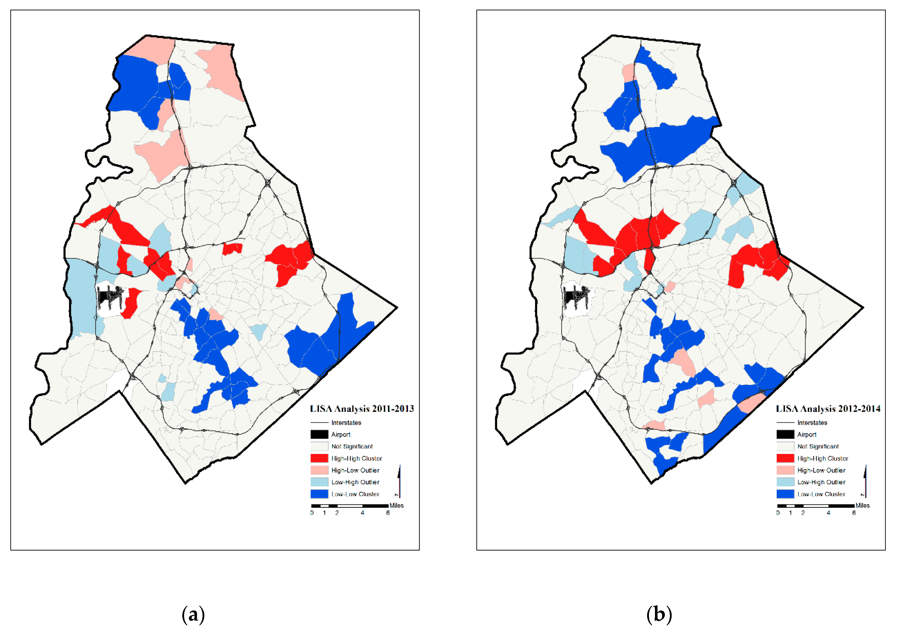
The geographic variation in prenatal hypertension rates per census tract in Mecklenburg County appears to reveal a non-random spatial pattern in the annual, two-year moving average, and three-year moving average (Figure 1, Figure 2 and Figure 3). This spatial pattern is formally tested with Moran’s I and LISA statistics. Given the geography of census tracts and the series of prenatal hypertension rates, we find the distribution of prenatal hypertension exhibits a significantly positive Moran’s I statistic for each of the eight data series tested (Table 2), indicating a level of positive spatial autocorrelation in hypertension across the county. The four categories of hot and cold spot census tracts are seen in the LISA maps of Mecklenburg County (Figure 4, Figure 5 and Figure 6) and the LISA results are documented in Table 3.
Overall, the incidence of prenatal hypertension does not happen randomly in the urban region under study. When we look at neighborhoods within the Mecklenburg County region, we find that hot spots tend to be loosely found in a crescent to the north of the county center throughout the study years. However, hot spots tend to shift to western portions of Mecklenburg County in 2013 and become more prominent in the east in 2014. These areas are known to be associated with the social geography of the region, particularly with a large proportion of African American and Hispanic populations, with lower educational attainment, and lower socio-economic status (i.e., higher poverty rates, lower household income, higher unemployment) [57]. Prenatal hypertension cold spots are mainly found in an area fanning out south from the county center as well as in the northern section of the county; this spatial pattern carries through the study period. Cold spots are found in neighborhoods with large presence of Caucasian populations, higher educational attainment, and higher socio-economic status [58]. Hot and cold spots fall in these areas with greater consistency as temporal windowing is applied to the yearly series, which suggests this is the discernable trend in prenatal hypertension once noise has been filtered out. Finally, while tracts that are outliers begin to fade away over time, hot and cold spots become more prominent. Hence, when noise caused by small-n annual statistics is controlled for, the same neighborhoods of the city continue to be separated by sharp health disparities epitomized by hot and cold spots in prenatal hypertension.
5. Discussion
Identifying the location of at-risk hot spot communities provides an opportunity to refine place-based health programs in urban regions with the use of temporal windowing. Geospatial analysis makes it feasible for local health departments to analyze their own data while complying with regulations and ethics related to protection of human subjects for public health surveillance and planning purposes. With a few procedures, existing data and publicly available databases can be leveraged by geocoding birth and death certificates to explore those data from different perspectives such that hot spots of census tracts can be pinpointed for further investigation, including for further confirmatory analysis of spatial epidemiology.
In the case of Mecklenburg County, chronic diseases such as hypertension continue to be cited as high priorities in the 2010–2018 Community Health Assessments (CHA) [59]. Although the CHA allows health departments a place to compile health priorities for the county, one major challenge health departments face is understanding the impact of initiatives aimed at reducing health disparities. With CHA conducted every 4 years, the county intends to track the overall indicator of women who have a history of one or more chronic diseases. However, Charlotte administrators have not tracked where hypertension hot spots are located, and whether these hot spots shrank or expanded over time.
In Charlotte, communities that have the highest priority in the CHA tend to have less education and income and live in neighborhoods which lack access to healthy food and safe places for recreation. Spatially, a crescent-shaped area of poverty and low-educational attainment has formed around the center city of Charlotte. These residents may also be exposed to risk factors that increase their chance for chronic disease. Our results demonstrated that once temporal windowing is used with the hypertension data, especially the two- and three-year windows, hot spot clusters emerged from these traditionally segregated communities in the Charlotte area. The benefit of tracking hypertension in Charlotte with Moran’s I and LISA analysis at census tracts is that it is possible to identify whether health departments achieve their goals from assessment to assessment. Although county level spatial aggregation continues to be in use routinely in most urban areas, this level of analysis precludes this type of surveillance and is rather ineffective to fully inform decision makers on where to target their efforts and on whether past efforts were successful.
Studying a series of spatial health data through a finer-scale analysis—such as the neighborhoods—allows a better understanding of local health outcomes and risk factors over time. Incorporating smaller geographies into a GIS can also aid health administrators by incorporating the location of hospital and medical facilities to address whether proximity influences the spread of the hot or cold spots. Moreover, U.S. Census and American Community Survey demographic data can be linked to see whether trends correlate with socio-economic conditions. Linking these data into the CHA will require collaboration with data stewards and adequate training of public health practitioners so that the benefits of using these data can be fully realized. In this way, a more tailored approach to surveying health priorities can be undertaken.
Our findings support that data spatially aggregated to the tract level lead to results that contribute to increased capacity to identify local clusters [60]. We also show that data stability and greater consistency in the significant spatial patterns can be obtained through a temporal windowing approach, which is an important achievement for strategic planning when rates are based on small numbers. Another type of models, known as Bayesian hierarchical models, have also been used to address sparseness in populations and cases, allowing for an adaptive smoothing approach [61]. This can, however, create overly smoothed maps, masking true risk distribution. The degree of smoothing used is a trade-off between high sensitivity and high specificity [62]. Prior research suggests that a numerator of 20 or more is needed to produce fairly stable estimates [63]. Also, it is well known that denominator data that rely on annual data sampling to apprehend the at-risk population (denominator)—such as annual American Community Survey data—is affected by large and spatially variable margins of error across the urban region. While some methods have been developed to provide unbiased estimates of statistics [64,65], many analyses continue to ignore this important and impactful data uncertainty [66].
We also acknowledge a key limitation in spatial analytics when dealing with aggregated data, such as census tracts. The possibility exists of having a Modifiable Areal Unit Problem [67], in the form of a scale effect or of a zoning effect. The scale effect arises when different results are attained due to variations in the scale of aggregation units. This implies that using census tracts rather than zip codes, for example, can lead to different findings. The zoning effects occur when a constant scale of analysis is used with a variation in the shape of aggregation units. This is the situation for census tracts, as well as zip codes and county boundaries. We did not test for scale or zoning effect because the study was to document how administrators can use confidential data. Further research is needed to understand which of the commonly used geographic scales is more useful for public health planning and under which conditions.
6. Conclusions
With tight state budgets limiting health department’s funds, using LISA on spatially aggregated secondary health data with a GIS provides for a targeted and more efficient approach to health resources planning, enabling monitoring of socio-economic determinants of health at a geographic scale commensurate with policy making and assessment. With the use of temporal windowing, administrators can reduce the effect of random noise while using a health indicators that are based on a small number of cases. The geographic tools used in this study are not intended to draw any causal conclusions about the spatial patterns that emerge from the analysis. Instead, they are powerful, effective, and robust for pattern detection and monitoring to enhance health administrator’s understanding of the processes that occur at the neighborhood or community level, such as census tracts, or whichever level administrators deem appropriate for the data to be aggregated too. Over time, the use of these tools will help local health departments identify how heath indicators change and what socio-demographic data associate with those changes.
We successfully demonstrated the application of this geospatial health analytics research design to the case of prenatal hypertension in the urban setting of Mecklenburg County, and because it is easy to reproduce, argue for its broad use in public health departments as part of their standard analytic toolbox. Tracking a system of sub-county data will allow public health officials in different urban contexts to benefit from our research by better understanding local health outcomes and risk factors over time. Incorporating these data into a collaborative urban network is advocated so that the benefits of using these data can be fully realized and identified challenges resolved.
Author Contributions
Conceptualization, D.Y., M.I., and J.-C.T.; methodology, D.Y. and J.-C.T.; formal Analysis, D.Y., M.I., and J.-C.T.; writing—original draft preparation, D.Y.; writing—review and editing, D.Y., M.I., and J.-C.T., visualization, D.Y.; supervision, M.I. and J.-C.T.
Funding
This research received no external funding.
Acknowledgments
We would like to thank Susan Long-Marin and Sara Lovett, and the Mecklenburg County Health Department for their support and cooperation with this project. We would also like to thank Paul Martin, from the Mecklenburg County Geospatial Information Services Department.
Conflicts of Interest
The authors declare no conflicts of interest.
Ethical Approval
(Blinded for review) Institutional Review Board.
References
- RESOLVE. The High Achieving Governmental Health Department in 2010 as the Community Chief Health StrateGISt; RESOLVE: Washington, DC, USA, 2014; Available online: http://www.resolv.org/site-healthleadershipforum/hd2020/ (accessed on 15 July 2015).
- Nagasko, E.; Waterman, B.; Reidhead, M.; Lian, M.; Gehlert, S. Measuring Subcounty Differences in Population Health Using Hospital and Census-Derived Data Sets: The Missouri ZIP Health Rankings Project. J. Public Health Manag. Pract. 2018, 4, 340–349. [Google Scholar] [CrossRef] [PubMed]
- Bemis, K.; Gray, S.; Patel, M.T.; Christiansen, D. Disproportionate emergency room use as an indicator of community health. Online J. Public Health Inf. 2016, 1, e9. [Google Scholar] [CrossRef]
- Lovett, D.A.; Poots, A.J.; Clements, J.T.C.; Green, S.A.; Samarasundera, E.; Bell, D. Using geographical information systems and cartograms as health services quality improvement tool. Spat. Spatio-Temporal Epidemiol. 2014, 10, 67–74. [Google Scholar] [CrossRef] [PubMed]
- Caprarelli, G.; Fletcher, S. A brief review of spatial analysis concepts and tools used for mapping, containment and risk modeling of infectious diseases and other illnesses. Parasitology 2014, 141, 581–601. [Google Scholar] [CrossRef] [PubMed]
- Berney, D.; Camponeschi, J.; Coon, M.; Creswell, P.D.; Schirmer, J.L.; Walsh, R. Using environmental public health tracking to identify community targets for public health actions in childhood lead poisoning in Wisconsin. J. Public Health Manag. Pract. 2015, 21, S80–S84. [Google Scholar] [CrossRef] [PubMed]
- Curtis, A.B.; Kothari, C.; Paul, R.; Connors, E. Using GIS and secondary data to target diabetes-related public health efforts. Public Health Rep. 2013, 128, 212–220. [Google Scholar] [CrossRef] [PubMed]
- Salinas, J.J.; Abdelbary, B.; Klass, K.; Tapia, B.; Sexton, K. Socioeconomic context and the food landscape in Texas: Results from hotspot analysis and border/non-border comparison of unhealthy food environments. Int. J. Environ. Res. Public Health 2014, 6, 5640–5650. [Google Scholar] [CrossRef] [PubMed]
- Brown, P.M.; Gonzales, M.; Dhaul, R.S. Cost of chronic disease in California: Estimates at the county level. J. Public Health Manag. Pract. 2015, 21, E10–E19. [Google Scholar] [CrossRef] [PubMed]
- Detres, M.; Lucio, R.; Vitucci, J. GIS as a community engagement tool: Developing a plan to reduce infant mortality risk factors. Matern. Child Health J. 2014, 18, 1049–1055. [Google Scholar] [CrossRef] [PubMed]
- Curtis, A.; Mills, J.; Agustin, L.; Cockburn, M. Confidentiality risks in fine scale aggregations of health data. Comput. Environ. Urban Syst. 2011, 1, 57–64. [Google Scholar] [CrossRef]
- Kanaroglou, P.; Delmelle, E.; Paez, A. Spatial Analysis in Health Geography; Routledge: New York, NY, USA, 2015. [Google Scholar]
- El Emnan, K.; Brown, A.; AbdelMalik, P. Evaluating predictors of geographic area population size cut-offs to manage re-identification risk. J. Am. Med. Inf. Assoc. 2009, 16, 256–266. [Google Scholar]
- Healy, M.A.; Gilliland, J.A. Quantifying the magnitude of environmental exposure misclassification when using imprecise address proxies in public health research. Spat. Spatio-Temporal Epidemiol. 2012, 3, 55–67. [Google Scholar] [CrossRef] [PubMed]
- Krefis, A.C.; Albrecht, M.; Kis, A.; Jagodzinski, A.; Augustin, M.; Augustin, J. Associations of Noise and Socioeconomic and -Demographic Status on Cardiovascular and Respiratory Diseases on Borough Level in a Large German City State. Urban Sci. 2017, 1, 27. [Google Scholar] [CrossRef]
- Waters, E.; Doyle, J. Evidence-based public health: Cochrane update. J. Public Health Med. 2003, 1, 72–75. [Google Scholar] [CrossRef]
- Boulos, M.N.K.; Curtis, A.; AbdelMalik, P. Musings on privacy issues in health research involving disaggregated geographic data about individuals. Int. J. Health Geogr. 2009, 8, 46. [Google Scholar] [CrossRef] [PubMed]
- Sherman, J.E.; Fetters, T.L. Confidentiality concerns with mapping survey data in reproductive health research. Stud. Fam. Plan. 2007, 4, 309–321. [Google Scholar] [CrossRef]
- Siffel, C.; Strickland, M.J.; Gardner, B.R.; Kirby, R.S.; Correa, A. Role of geographic information systems in birth defects surveillance and research. Birth Defects Res. A Clin. Mol. Teratol. 2006, 11, 825–833. [Google Scholar] [CrossRef] [PubMed]
- Matthews, S.A.; Moudon, A.V.; Daniel, M. Work group II: Using Geographic Information Systems for enhancing research relevant to policy on diet, physical activity, and weight. Am. J. Prev. Med. 2009, 4, S171–S176. [Google Scholar] [CrossRef]
- Smolders, R.; Casteleyn, L.; Joas, R.; Schoeters, G. Human biomonitoring and the INSPIRE directive: Spatial data as link for environment and health research. J. Toxicol. Environ. Health B Crit. Rev. 2008, 8, 646–659. [Google Scholar] [CrossRef]
- Foley, R. Assessing the applicability of GIS in a health and social care setting: Planning services for informal careers in East Sussex. Engl. Soc. Sci. Med. 2002, 1, 79–96. [Google Scholar] [CrossRef]
- McKenzie, G.; Janowicz, K.; Seidl, D. Geo-Privacy beyond Coordinates. In Geospatial Data in a Changing World: Selected Papers of the 19th AGILE Conference on Geographic Information Science; Sarjakoski, T., Santos, M., Sarjakoski, L., Eds.; Springer International Publishing: Cham, Switzerland, 2016; pp. 157–175. [Google Scholar]
- Centers for Disease Control and Prevention. HIPAA privacy rule and public health: Guidance from CDC and the US Department of Health and Human Services. MMWR Morb. Mortal. Wkly. Rep. 2003, 52, 1–20. [Google Scholar]
- Office of Clinical Research. Guidance Regarding Methods for De-identification of Protected Health Information in Accordance with the Health Insurance Portability and Accountability Act (HIPAA) Privacy Rule; United States Department of Health and Human Services: Washington, DC, USA, 2012. [Google Scholar]
- VanWey, L.K.; Rindfuss, R.R.; Gutmann, M.P.; Entwisle, B.; Balk, D.L. Confidentiality and spatially explicit data: Concerns and challenges. Proc. Natl. Acad. Sci. USA 2005, 102, 15337–15342. [Google Scholar] [CrossRef] [PubMed] [Green Version]
- El Emam, K.; Jonker, E.; Arbuckle, L.; Malin, B. Correction: A systematic review of re-identification attacks on health data. PLoS ONE 2015, 4, e0126772. [Google Scholar] [CrossRef] [PubMed]
- Seidl, D.; Paulus, G.; Jankowski, P.; Regenfelder, M. Spatial obfuscation methods for privacy protection of household-level data. Appl. Geogr. 2015, 63, 253–263. [Google Scholar] [CrossRef]
- Acevedo-Garcia, D.; McArdle, N.; Hardy, E.F.; Crisan, U.I.; Romano, B.; Norris, D.; Baek, M.; Reece, J. The child opportunity index: Improving collaboration between community development and public health. Health Aff. 2014, 11, 1948–1957. [Google Scholar] [CrossRef] [PubMed]
- Boulos, M.N.K. Towards evidence-based, GIS-driven national spatial health information infrastructure and surveillance services in the United Kingdom. Int. J. Health Geogr. 2004, 1, 1–50. [Google Scholar] [CrossRef]
- Chun, Y.; Griffith, D.A. Spatial Statistics & Geostatistics; Sage: Los Angeles, CA, USA, 2013. [Google Scholar]
- Pfeiffer, D.; Robinson, T.P.; Stevenson, M.; Stevens, K.B.; Rogers, D.C.; Clements, A.C. Spatial Analysis in Epidemiology; Oxford University Press: New York, NY, USA, 2008. [Google Scholar]
- Stoto, M.A. Population Health in the Affordable Care Act Era; Academy Health: Washington, DC, USA, 2013; Available online: https://www.academyhealth.org/files/AH2013pophealth.pdf (accessed on 15 July 2015).
- Vest, J.R.; Issel, L.M. Factors related to public health data sharing between local and state health departments. Health Serv. Res. 2014, 1, 373–391. [Google Scholar] [CrossRef]
- Meltzer, D.O.; Chung, J.W. The population value of quality indicator reporting: A framework for prioritizing health care performance measures. Health Aff. 2014, 33, 132–139. [Google Scholar] [CrossRef]
- Lyseen, A.K.; Nohr, C.; Sorensen, E.M.; Gudes, O.; Geraghty, E.M.; Shaw, N.T.; Bivona-Tellez, C.; IMIA Health GIS Working Group. A review and framework for categorizing current research and development in health related geographical information systems (GIS) studies. Yearb. Med. Inform. 2014, 1, 110–124. [Google Scholar]
- Geographic Research, Inc. Census 2012 Data; Geographic Research, Inc.: New York, NY, USA, 2015. [Google Scholar]
- Brondolo, E.; Love, E.E.; Pencile, M.; Schoenthaler, A.; Ogedegbe, G. Racism and hypertension: A review of the empirical evidence and implications for clinical practices. Am. J. Hypertens. 2011, 24, 518–529. [Google Scholar] [CrossRef]
- Committee on Practice-Obstetics. Gestational hypertension and preeclampsia. ACOG Practice Bulletin No. 202. American College of Obstetricians and Gynecologists. Obstet. Gynecol. 2019, 133, e1–e25. [Google Scholar] [CrossRef] [PubMed]
- Grady, S.C.; Ramirez, I.J. Mediating medical risk factors in the residential segregation and low birthweight relationship by race in New York City. Health Place 2008, 14, 661–677. [Google Scholar] [CrossRef] [PubMed]
- Hauspurg, A.; Parry, S.; Mercer, B.M.; Grobman, W.; Hatfield, T.; Silver, R.M.; Parker, C.B.; Haas, D.M.; Iams, J.D.; Saade, G.R.; et al. Blood pressure trajectory and category and risk of hypertensive disorders of pregnancy in nulliparous women. Am. J. Obstet. Gynecol. 2019, in press. [Google Scholar] [CrossRef] [PubMed]
- Olson-Chen, C.; Seligman, N.S. Hypertensive Emergencies in Pregnancy. Crit. Care Clin. 2016, 32, 29–41. [Google Scholar] [CrossRef] [PubMed]
- Gillon, T.E.; Pels, A.; von Dadelszen, P.; Magee, L.A. Hypertensive disorders of pregnancy: A systematic review of International clinical practice guidelines. PLoS ONE 2014, 9, e113715. [Google Scholar] [CrossRef] [PubMed]
- Nelson, E.J.; Shacham, E.; Boutwell, B.B.; Rosenfeld, R.; Schootman, M.; Vaughn, M.; Lewis, R. Childhood lead exposure and sexually transmitted infections: New evidence. Environ. Res. 2015, 143, 131–137. [Google Scholar] [CrossRef] [PubMed]
- Edwards, S.E.; Strauss, B.; Miranda, M.L. Geocoding large population-level administrative datasets at highly resolved spatial scales. Trans. GIS 2014, 4, 586–603. [Google Scholar] [CrossRef] [PubMed]
- Toledo, L.; Codeco, C.T.; Bertoni, N. Putting respondent-driven sampling on the map: Insights from Rio de Janeiro, Brazil. J. Acquir. Immune Defic. Syndr. 2011, 57, S136–S143. [Google Scholar] [CrossRef]
- Anselin, L. Local indicators of spatial association—LISA. Geogr. Anal. 1995, 2, 93–115. [Google Scholar] [CrossRef]
- Xia, J.; Cai, S.; Zhang, H.; Lin, W.; Fan, Y.; Qiu, J.; Sun, L.; Chang, B.; Nie, S. Spatial, temporal, and spatiotemporal analysis of malaria in Hubei Province, China from 2004–2011. Malar. J. 2015, 14, 1–10. [Google Scholar] [CrossRef]
- Abbas, T.; Younus, M.; Muhammad, S.A. Spatial cluster analysis of human cases of Crimean Congo hemorrhagic fever reported in Pakistan. Infect. Dis. Poverty 2015, 4, 9. [Google Scholar] [CrossRef] [PubMed]
- Zhang, J.; Yin, F.; Zhang, T.; Yang, C.; Zhang, X.; Feng, Z.; Li, X. Spatial analysis on human brucellosis incidence in mainland China: 2004–2010. BMJ Open 2014, 4, e004470. [Google Scholar] [CrossRef] [PubMed]
- Zhu, B.; Fu, Y.; Liu, J.; Mao, Y. Notifiable sexually transmitted infections in China: Epidemiologic trends and spatial changing patterns. Sustainability 2017, 9, 1784. [Google Scholar] [CrossRef]
- Zhu, B.; Liu, J.; Fu, Y.; Zhang, B.; Mao, Y. Spatio-temporal epidemiology of viral hepatitis in China (2003–2015): Implications for prevention and control policies. Int. J. Environ. Res. Public Health 2018, 15, 661. [Google Scholar] [CrossRef]
- Anselin, L.; Syabri, I.; Kho, Y. GeoDa: An Introduction to Spatial Data Analysis. Geogr. Anal. 2006, 38, 5–22. [Google Scholar] [CrossRef]
- Getis, A.; Ord, J.K. The analysis of spatial association by use of distance statistics. Geogr. Anal. 1992, 3, 189–206. [Google Scholar] [CrossRef]
- Anselin, L. The Moran scatterplot as an ESDA tool to assess local instability in spatial association. In Spatial Analytical Perspectives on GIS in Environmental and Socio-Economic Sciences; Fischer, M., Scholten, H., Unwin, D., Eds.; Taylor and Francis: London, UK, 1997; pp. 111–215. [Google Scholar]
- Bailey, T.C.; Gatrell, A.C. Interactive Spatial Data Analysis; Wiley: Hoboken, NJ, USA, 1995. [Google Scholar]
- Charlotte/Mecklenburg Quality of Life Explorer. 2019. Available online: https://mcmap.org/qol/#15/ (accessed on 15 July 2019).
- Charlotte/Mecklenburg Quality of Life Explorer. 2019. Available online: https://mcmap.org/qol/#/p1/ https://mcmap.org/qol/#14/ (accessed on 15 July 2019).
- Mecklenburg County Health Department. Mecklenburg County Community Health Assessment. 2018. Available online: https://www.mecknc.gov/HealthDepartment/HealthStatistics/Pages/Community-Health-Assessment.aspx (accessed on 13 July 2019).
- Gregorio, D.I.; Dechello, L.M.; Samociuk, H.; Kulldorff, M. Lumping or splitting: Seeking the preferred areal unit for health geography studies. Int. J. Health Geogr. 2005, 4, 6. [Google Scholar] [CrossRef]
- Beale, L.; Abellan, J.J.; Hodgson, S.; Jarup, L. Methodologic issues and approaches to spatial epidemiology. Environ. Health Perspect. 2008, 116, 1105–1110. [Google Scholar] [CrossRef]
- Elliott, P.; Wartenberg, D. Spatial epidemiology: Current approaches and future challenges. Environ. Health Perspect. 2004, 9, 998–1006. [Google Scholar] [CrossRef]
- Shah, G.H. A Guide to Designating Geographic Areas for Small Area Analysis in Public Health: Using Utah’s Example; NAHDO-CDC Cooperative Agreement Project; NAHDO-CDC Cooperative: Salt Lake City, UT, USA, 2005. [Google Scholar]
- Jung, P.H.; Thill, J.-C.; Issel, M. Spatial Autocorrelation and Data Uncertainty in the American Community Survey: A Critique. Int. J. Georgr. Inf. Sci. 2019, 6, 1155–1175. [Google Scholar] [CrossRef]
- Jung, P.H.; Thill, J.-C.; Issel, M. Spatial Autocorrelation Statistics of Areal Prevalence Rates under High Uncertainty in Denominator Data. Geogr. Anal. 2018, in press. [Google Scholar] [CrossRef]
- Major, E.; Delmelle, E.; Delmelle, E. SNAPScapes: Using geodemographic segmentation to classify the food access landscape. Urban Sci. 2018, 2, 71. [Google Scholar] [CrossRef]
- Gatrell, A.C.; Bailey, T.C.; Diggle, P.J.; Rowlingson, B.S. Spatial point pattern analysis and its application in geographical epidemiology. Trans. Inst. Br. Geogr. 1996, 21, 256–274. [Google Scholar] [CrossRef]
Figure 1.
Annual prenatal hypertension rate per 1000 births in Mecklenburg County, NC for (a) 2011 (b) 2012 (c) 2013 (d) 2014.
Figure 1.
Annual prenatal hypertension rate per 1000 births in Mecklenburg County, NC for (a) 2011 (b) 2012 (c) 2013 (d) 2014.
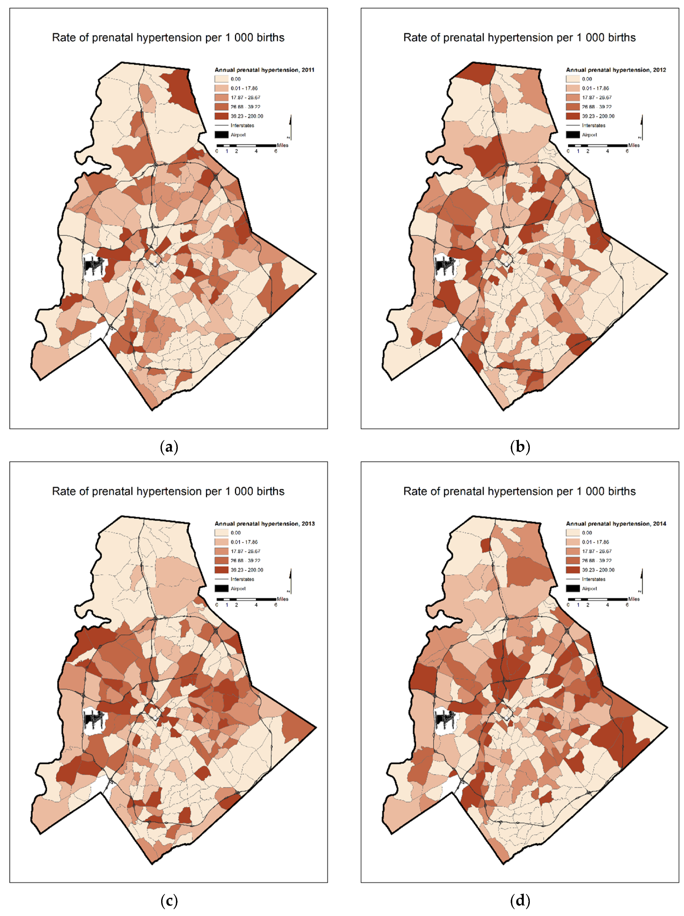
Figure 2.
Prenatal hypertension rate per 1000 births: two-year moving average in Mecklenburg County, NC for (a) 2011–2012 (b) 2012–2013 (c) 2013–2014.
Figure 2.
Prenatal hypertension rate per 1000 births: two-year moving average in Mecklenburg County, NC for (a) 2011–2012 (b) 2012–2013 (c) 2013–2014.
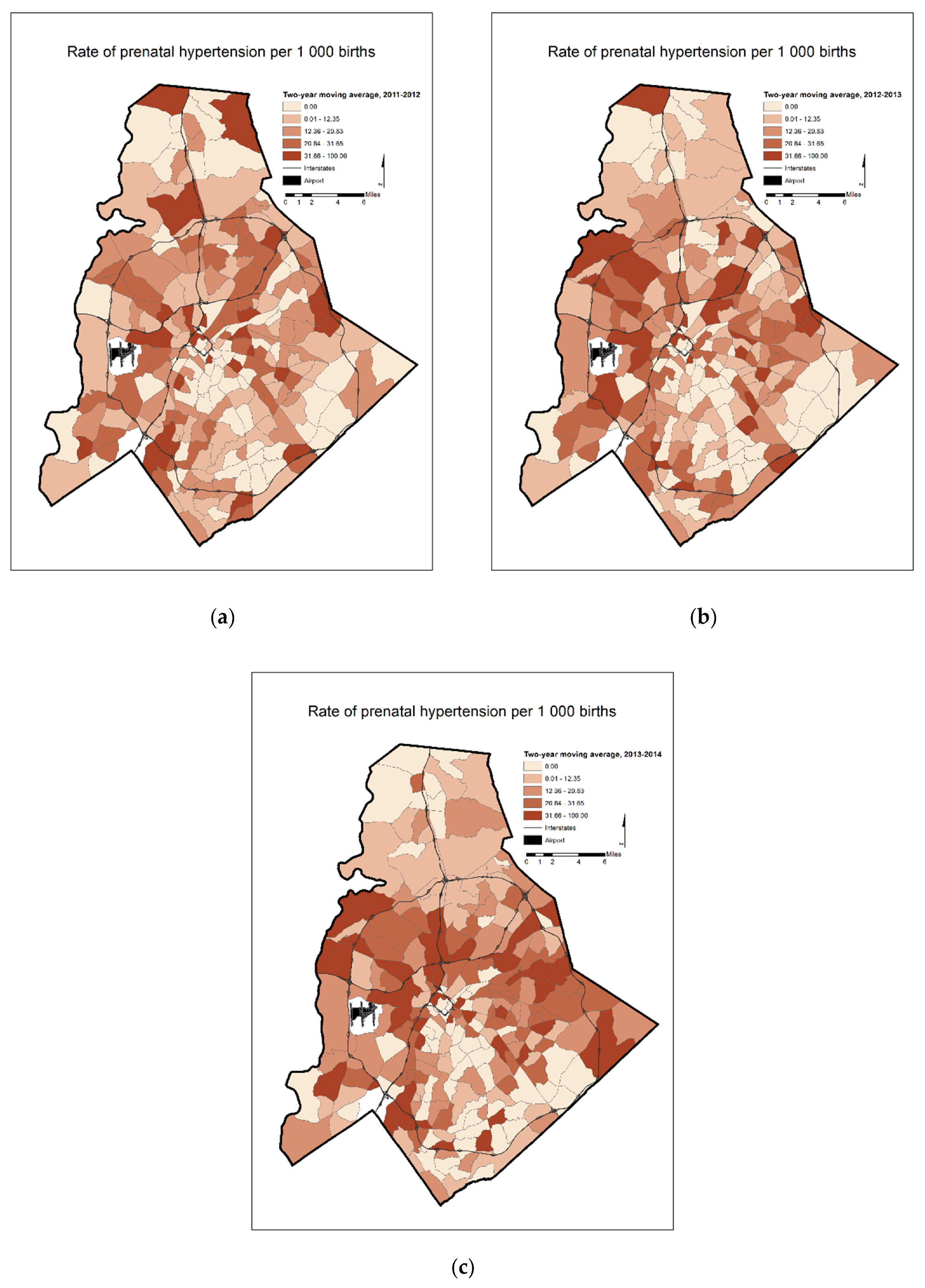
Figure 3.
Prenatal hypertension rate per 1000 births: three-year moving average in Mecklenburg County, NC for (a) 2011–2013 (b) 2012–2014.
Figure 3.
Prenatal hypertension rate per 1000 births: three-year moving average in Mecklenburg County, NC for (a) 2011–2013 (b) 2012–2014.
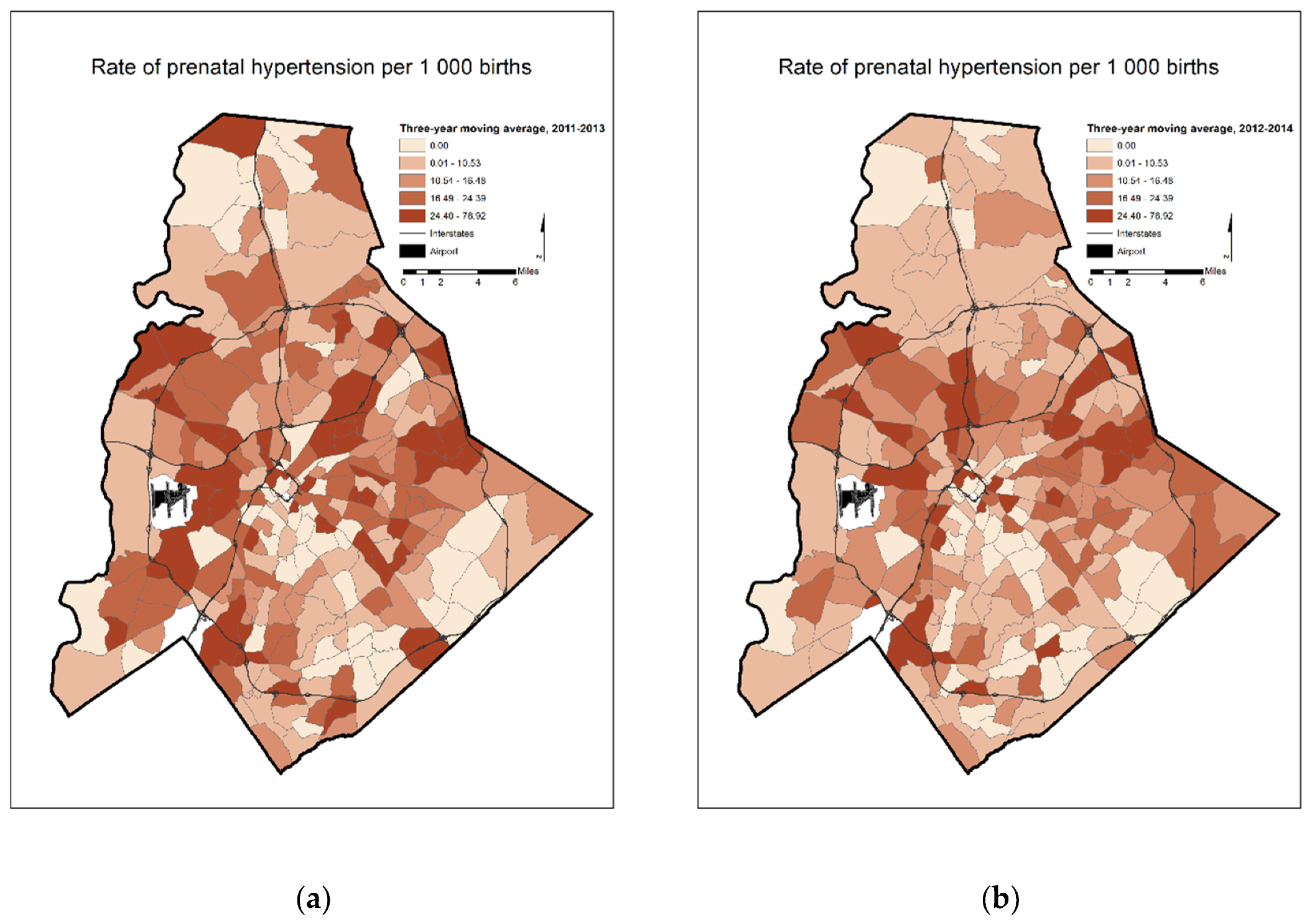
Figure 4.
LISA results on annual prenatal hypertension rates in Mecklenburg County, NC for (a) 2011 (b) 2012 (c) 2013 (d) 2014.
Figure 4.
LISA results on annual prenatal hypertension rates in Mecklenburg County, NC for (a) 2011 (b) 2012 (c) 2013 (d) 2014.
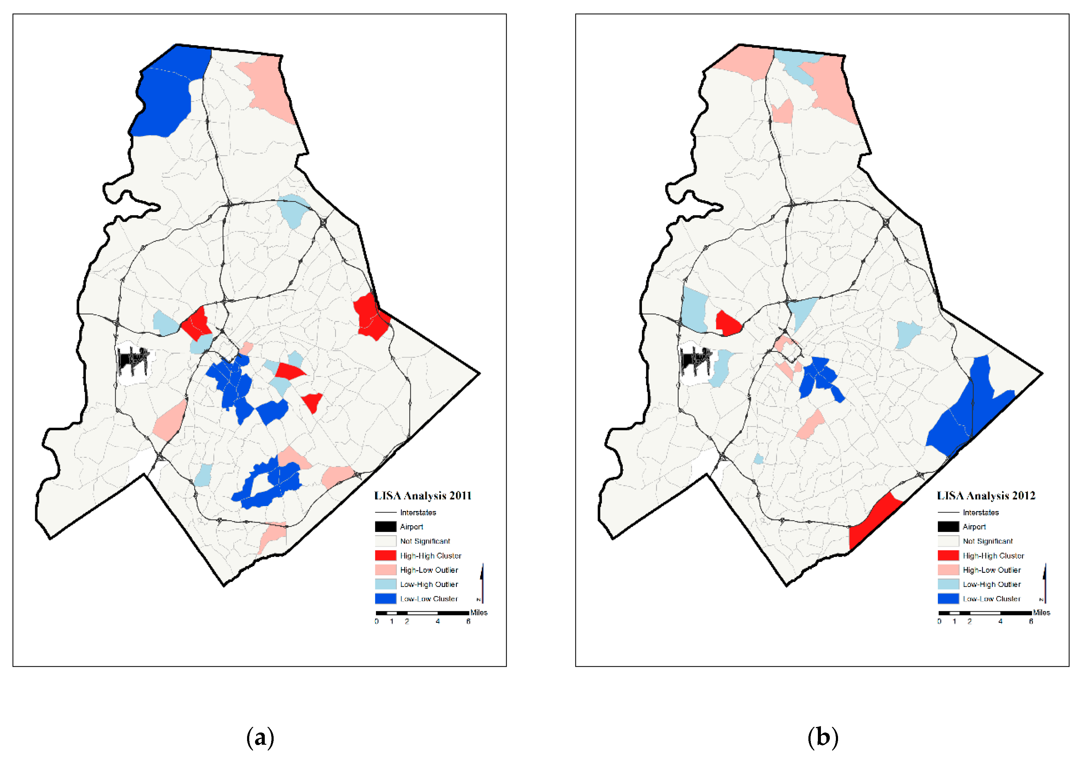
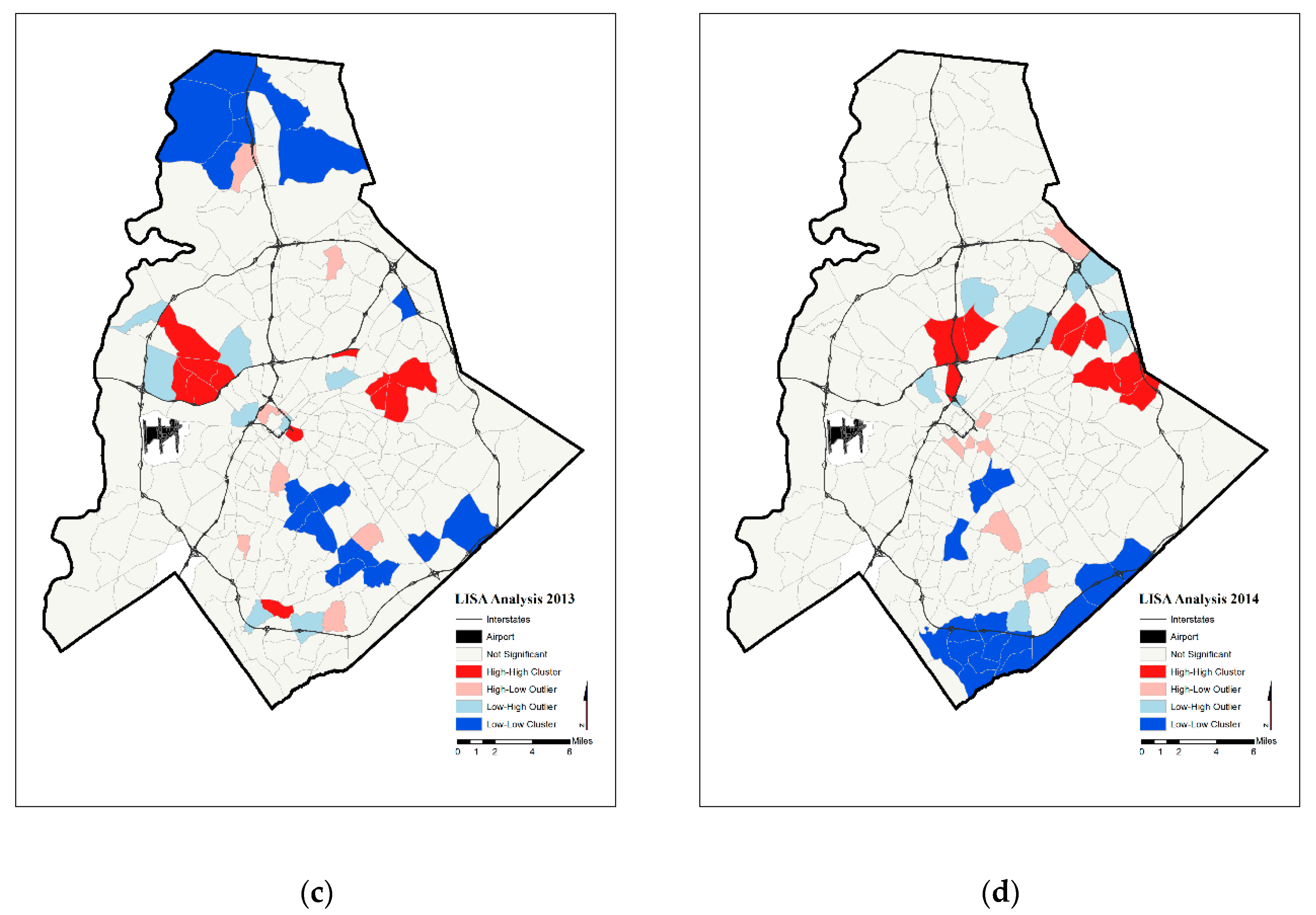
Figure 5.
LISA results on prenatal hypertension rate two-year moving averages in Mecklenburg County, NC for (a) 2011–2012 (b) 2012–2013 (c) 2013–2014.
Figure 5.
LISA results on prenatal hypertension rate two-year moving averages in Mecklenburg County, NC for (a) 2011–2012 (b) 2012–2013 (c) 2013–2014.
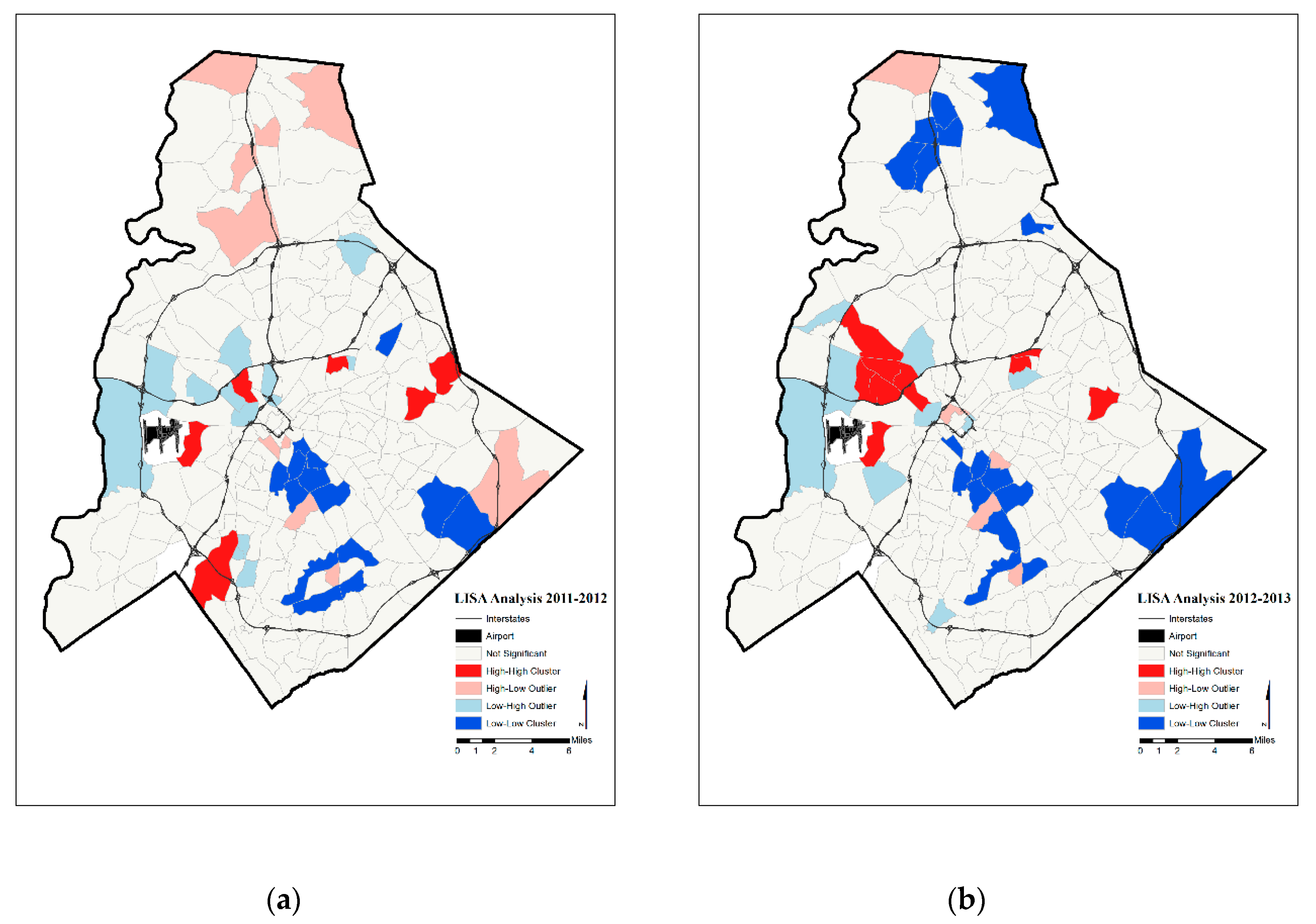
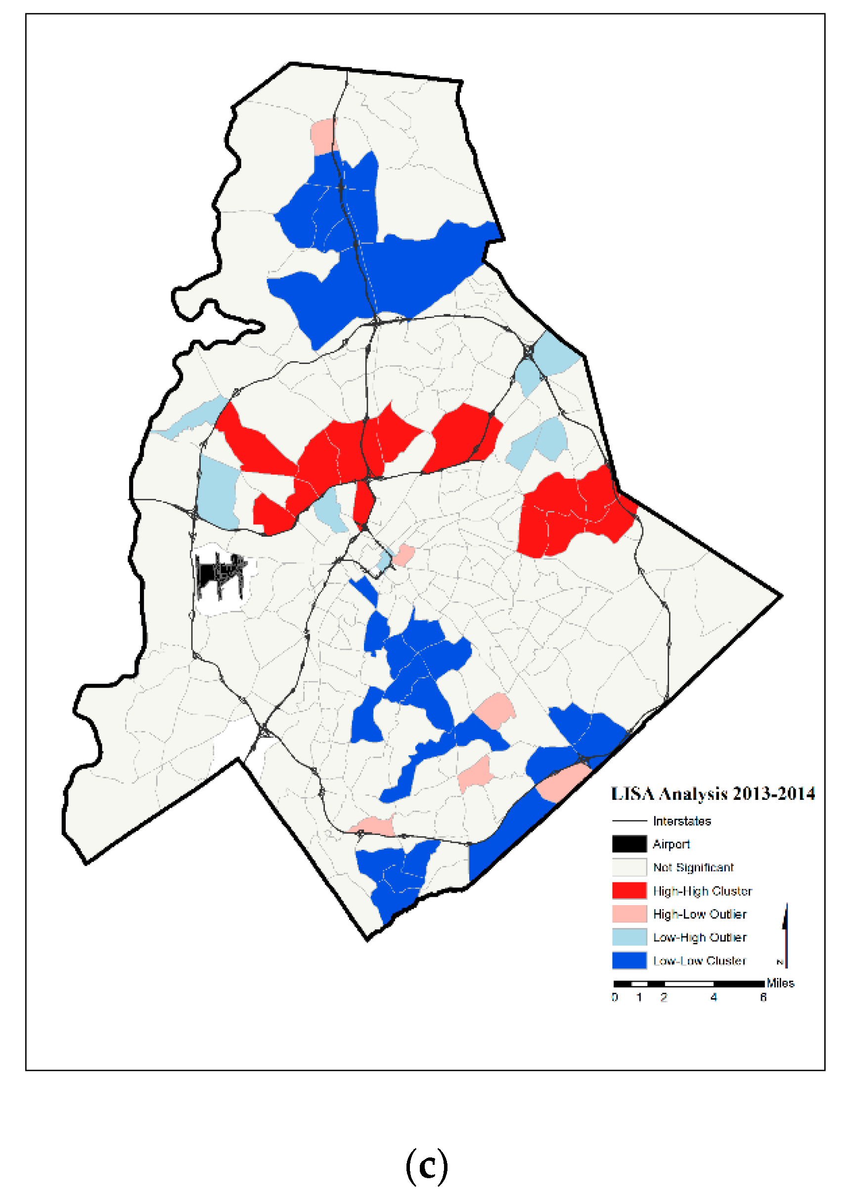
Figure 6.
LISA results on prenatal hypertension rate three-year moving averages in Mecklenburg County, NC for (a) 2011–2013 (b) 2012–2014.
Figure 6.
LISA results on prenatal hypertension rate three-year moving averages in Mecklenburg County, NC for (a) 2011–2013 (b) 2012–2014.

Table 1.
Relationship of high and low rates in focal and surrounding census tracts as revealed though LISA analysis.
Table 1.
Relationship of high and low rates in focal and surrounding census tracts as revealed though LISA analysis.
| High Rates in Focal Census Tract | Low Rates in Focal Census Tract | |
|---|---|---|
| High Average Rates in Surrounding Census Tracts | “Hot spots” | Spatial outlier |
| Low Average Rates in Surrounding Census Tracts | Spatial outlier | “Cold spots” |
Table 2.
Moran’s I statistic by year.
| Year(s) | Moran’s I Statistic |
|---|---|
| 2011 | 0.067 |
| 2012 | 0.071 |
| 2013 | 0.095 |
| 2014 | 0.068 |
| 2011–2012 | 0.037 |
| 2012–2013 | 0.067 |
| 2013–2014 | 0.010 |
| 2011–2013 | 0.106 |
| 2012–2014 | 0.108 |
All years significant at p < 0.001.
Table 3.
LISA results.
| Year | Significant Tracts | Hot Spot | Cold Spot | |
|---|---|---|---|---|
| Annual Prenatal Hypertension Rates | 2011 | 36 | 6 | 17 |
| 2012 | 23 | 2 | 8 | |
| 2013 | 45 | 12 | 18 | |
| 2014 | 41 | 9 | 17 | |
| Two-Year Moving Average Prenatal Hypertension Rates | 2011–2012 | 43 | 6 | 14 |
| 2012–2013 | 43 | 10 | 19 | |
| 2013–2014 | 52 | 13 | 26 | |
| Three-Year Moving Average Prenatal Hypertension Rates | 2011–2013 | 50 | 12 | 22 |
| 2012–2014 | 49 | 11 | 22 |
© 2019 by the authors. Licensee MDPI, Basel, Switzerland. This article is an open access article distributed under the terms and conditions of the Creative Commons Attribution (CC BY) license (http://creativecommons.org/licenses/by/4.0/).
Share and Cite
MDPI and ACS Style
Yonto, D.; Issel, L.M.; Thill, J.-C. Spatial Analytics Based on Confidential Data for Strategic Planning in Urban Health Departments. Urban Sci. 2019, 3, 75. https://doi.org/10.3390/urbansci3030075
AMA Style
Yonto D, Issel LM, Thill J-C. Spatial Analytics Based on Confidential Data for Strategic Planning in Urban Health Departments. Urban Science. 2019; 3(3):75. https://doi.org/10.3390/urbansci3030075
Chicago/Turabian StyleYonto, Daniel, L. Michele Issel, and Jean-Claude Thill. 2019. "Spatial Analytics Based on Confidential Data for Strategic Planning in Urban Health Departments" Urban Science 3, no. 3: 75. https://doi.org/10.3390/urbansci3030075