Article

Influence of the Natural and Built Environment on Personal Exposure to Fine Particulate Matter (PM2.5) in Cyclists Using City Designated Bicycle Routes

1
Department of Geography, Western University, London, ON N6A 6C2, Canada
2
Department of Civil and Environmental Engineering, University of Windsor, Windsor, ON N9B 3P4, Canada
*
Author to whom correspondence should be addressed.
Urban Sci. 2018, 2(4), 120; https://doi.org/10.3390/urbansci2040120
Submission received: 29 October 2018 / Revised: 5 December 2018 / Accepted: 14 December 2018 / Published: 19 December 2018

Abstract

:
Urban cyclists are exposed to many traffic-related air pollutants including particulate matter (PM) that may increase vulnerability to health effects. This study investigates second-by-second personal exposure to PM2.5 (fine particulate matter that is 2.5 microns in diameter and less) along bicycle commuting paths, and assesses elements of the natural and built environment for the relative importance of these factors in understanding the variability in PM2.5 personal exposure. Urban cyclists were carrying high resolution PM2.5 monitors (placed in a backpack) in combination with portable GPS trackers to provide a spatial identity to each one-second pollutant measurement. The results of this study indicate that daily averages of PM2.5 concentrations from all bicycle routes were weakly correlated with meteorological variables, however, a strong influence of regional levels of PM2.5 was observed. Geospatial analysis of PM2.5 personal exposure concentrations showed a considerable variation within routes, correlated with land use (with lower concentrations in parks and higher in industrial areas) and clustered at four areas: busiest bridge, heavily trafficked road segments, the downtown urban core, and two construction sites. This study has found many incidences of personal exposure to PM2.5 exceeding the provincial guidelines for healthy activity (e.g., very poor (PM2.5 > 91 μg/m3) pollution concentrations are clustered in three regions: approaching the bridge in the west part of the city; the downtown urban core; and two under construction spots), which suggests behavioural and infrastructure modifications in balancing the health benefits of cycling with the environmental exposure to air pollutants.

1. Introduction

Cycling is becoming an increasingly popular commuting choice for North Americans [1,2]. Many cyclists and promoters of ‘active transport’ perceive cycling to be the healthier commute option compared to motorized transport [3,4,5,6]. However, when in close proximity to vehicular traffic, cyclists may be exposed to levels of air pollution (e.g., particulate matter ‘PM2.5’), which are potentially hazardous to their health [7,8]. PM2.5 is of special concern to cyclists as it is considered a respirable fraction since it can penetrate deeper into the lungs than larger particulates and thus capable of damaging the gas exchange surface directly [9]. Exposure is compounded with increased breathing rate and intensity [10] and extra time spent commuting compared to those who travel by motor vehicles. The natural environment, especially meteorological conditions, is known to significantly contribute to variation in PM2.5 concentration. Specifically, active personal measurements of PM2.5 increase with temperature but are not influenced by precipitation [11]. Wind has also been found to significantly reduce PM2.5 measurements [12,13,14,15], accounting for 18% of PM2.5 variation in one study [16], or had no effect [11,17]. A vertical gradient in PM2.5 distribution exists for both intraurban elevation [18] as well as on the microscale, requiring personal exposure equipment to sample air near the breathing zone for accurate measurements [12]. Although meteorological parameters have been shown to influence dispersion, one study [19] could not find any significant influence on the elemental composition of PM2.5.
Although much of the ambient PM2.5 is a result of long distance transport [6] of often unknown sources, the built environment can generate or influence the distribution of PM2.5 in local scales, especially in urban centres. Mutually inclusive categories of the built environment known to influence PM2.5 concentrations include infrastructure responsible for traffic, urban form, and land use. In Toronto, motor vehicle-related emissions including road salt were estimated to be responsible for about 40% of observed PM2.5 [20]. Daily PM2.5 measurements were influenced by distance from arterial roads [18] with a modest, but significant gradient based upon traffic volumes [21] There is, however, disagreement over how much traffic accounts for differences in personal exposure to PM2.5. Increased particulate readings were observed, but not quantified, around traffic-lighted intersections attributing this change to emissions occurring when vehicles slow and accelerate [22] Urban form, consisting of building configurations and road layout, has also been shown to influence PM2.5 distribution. The street canyon effect, where the shape and height of buildings and proximity to the road influences airflow, has been shown to: (1) have an effect on PM2.5 readings depending on the direction of wind [15], (2) influence daily PM2.5 measurements in Hong Kong [23] and (3) have no effect in London, UK [24]. Land use has not often been correlated with personal exposure measurements of PM2.5 and there have been conflicting reports of their influence on intraurban PM2.5 variability. High resolution personal exposure to PM3, a particulate matter fraction very similar to PM2.5, was found to be fairly homogenous across land use categories over a 20 km bicycle route in Vancouver, Canada [11]. Similarly, distance from industrial PM2.5 point source emissions did not predict daily sum PM2.5 counts [18]. In contrast, daily PM2.5 measurements in Hong Kong were found to vary depending on the sample location’s predominant land use, with the lowest found in industrial, moderate in commercial and highest in residential; however statistical analyses were not conducted to delineate the influence of individual land uses potentially nullifying the significance of land use as a predictor of PM2.5 distribution.
Very few studies have examined personal exposure to air pollution of cyclists, with the majority of previous research taking place in European towns and cities. Even fewer studies attempt to account for the specific environmental elements that contribute to the variation in pollutants such as PM2.5. To our knowledge, no previous study has assessed both elements of the natural environment and built environment for the relative importance of these factors in accounting for variability in PM2.5 personal exposure to cyclists [25]. In an attempt to fill gaps in knowledge, this study examines environmental influences on personal exposure to PM2.5 among cyclists in London, Ontario, a mid-sized Canadian city with a population of 383,822 in 2016 [26]. Commuting cyclists are generally unable to complete their entire journeys along segregated bike paths (away from roads) and often must navigate a variety of land uses, built environments and urban forms, each with different potential for air pollution concentrations. Previous literature has found considerable variation and conflicting results for predictors of personal exposure of cyclists to PM2.5, suggesting that the conclusions of personal monitoring studies cannot be uncritically transferred to different geographical locations [27]. This study aims to map and identify the urban characteristics of PM2.5 hotspots, defined here in two ways: as the top 1% of readings, and alternatively as any measurements within the highest health bracket determined by the Ontario Ministry of the Environment (PM2.5 > 91 μg/m3). The larger purpose of the study is to create a predictive model for PM2.5 exposure along a bicycle path by incorporating the highest correlated elements into a linear regression model in order to provide evidence for future route planning or route modification.
The elements of the built environment examined in this study were selected based upon their known contribution to intra-urban PM2.5 variability from previous research. Traffic-related variables including path type, speed limit, traffic, and distances to various traffic-related elements (nearest arterial road, intersection, etc.) were selected as vehicle emissions have been shown to contain PM2.5 [20]. Truck and bus routes were also selected as PM2.5 has been shown to be an especially good proxy for diesel engine emissions [12]. Street trees have been shown to reduce ultrafine particle (UFP) from roadways [28] but have not been examined for their role in the PM2.5 distribution and are thus included in this analysis. Land use and measures of land use mix were also considered as they have been shown to influence personal exposure to PM2.5 [13]. Buffer distances for land use variables were based on previous linear regression models for PM2.5 [17] as no a priori known gradient for PM2.5 concentration decay has been observed from major roads [29].
This case study uses a high resolution PM2.5 monitor in combination with a portable GPS tracker to provide a spatial account of the specific environmental elements that contribute to the variation in personal exposure to PM2.5 of commuting cyclists. Specifically, this case study aims to locate PM2.5 ‘hotspots’ along bicycle commuting paths and to assess relationships between characteristics of the natural and built environment and the variability in cyclists’ PM2.5 personal exposure. A better understanding of environmental correlates with air pollution exposures may help municipal policymakers, planners, and engineers develop more effective policies and/or infrastructural interventions for mitigating negative health impacts of air pollution in support of healthy, physically active modes of transportation such as cycling.

2. Methods

2.1. Route Selection

To create a representative sample of the entire bicycle path network in the city of London, Ontario, five routes totaling 64 km, or 28.3% of the 226 km network of municipally-designated bicycle paths were identified. These routes were chosen from different geographic areas within the city limits by the research team within a geographic information system (GIS) based upon the mixture of land uses located within 100 m of the path (Table 1). Land uses were identified using a GIS file of parcel-level land uses provided by the City of London and area for each land use tabulated using the intersect function for 100 m buffers. Study routes had similar land use environments to those found throughout the entire bicycling network (+2.5%) and loop around and come back to starting point to capture all possible directions in each trip. Besides attempting to maximize the mix of land uses experienced by a cyclist, selected routes were also designed to represent potential commuting routes of hypothetical cyclists, with circuits stretching between the downtown commercial core and suburban residential districts that may include short segments of streets without bicycle paths (i.e., must cycle on road). The northern route includes residential and recreational areas around Western University, whereas the western route is mostly residential in nature. The routes from southern and southeastern areas are generally commercial and industrial with busier, high-traffic streets with heavy-duty vehicles
Study participants included 5 graduate students recruited from the University of Western Ontario (UWO); all participants had prior experience cycling within the city. To simulate the conditions found during a normal morning commute, five simultaneous trials were run by volunteer cyclists weekdays between 7 AM and 9 AM (in June). In addition, this time period has been shown historically to correspond to one of the pollution peaks in the diurnal cycle of ambient PM2.5, presumably from anthropogenic commuting activity at this time [30]. To minimize subtle temporal changes in ambient pollution readings between these two study hours, participants were asked to alternate direction of routes daily. The study was approved by the UWO Non-Medical Research Ethics Board (#16455S).

2.2. Instrumentation and Data Collection

Particulate matter with an aerodynamic diameter of less than 2.5 μm was continuously measured by photometric sensing and recorded by pDR-1500 Personal Data Recorders (Thermo Fisher Scientific, Waltham, MA, USA) with an averaging time of one second. The pDR-1500 units were placed in backpacks with a rubber tube extending from the device intake to the shoulder strap where the inlet was fixed to ensure consistent sampling at a level representative of the breathing zone. Assuming a travel speed of 20 km/h, a sample measurement was obtained approximately every 6 m. Cyclists were also given Garmin (E-TREX) GPS devices to provide a spatial identity to each one-second pollutant measurement from the pDR-1500 by joining the data through common ‘time stamps’. Units were time synchronized and tested before and after the experiment to ensure proper intra-comparison.

2.3. Data Sources

Land use data was obtained from the City of London, Ontario. The number of street trees, traffic counts by street segment, the path type, intersections and traffic lights, the footprints of all structures, roads with speed limits, bus routes and truck routes were obtained from the City of London Geomatics Division. Hourly meteorological conditions (temperature (°C), relative humidity (%), wind direction (degrees from geographic north), and wind speed (km/h)) measured at the London Station between 7 AM and 9 AM for the five study days were obtained from the Ontario Ministry of the Environment and Climate Change (2011).

2.4. Data Analysis

To prepare data for analysis, GPS derived location data from the five study routes were combined into a single 64 km path and broken into 1 m segments along the centre of the pre-designated route in ArcMap software. To identify how PM2.5 concentrations varied in different locations, each PM2.5 measurement logged with the pDR-1500 s was spatially referenced by linking them to the data points captured with the GPS device according to the time record on both instruments. Each pollution point was then assigned to the nearest 1 m segment within the search radius of 25 m using a spatial join tool (see, Figure 1).
The 25 m search buffer, which encapsulates 68% of all points, was a compromise between fidelity to the atmosphere around the 1 m route segments and sample size. Only very marginal gains in sample size (2%) were found using a much larger 50 m buffer. Conversely, a 10 m buffer captures 64% of points, and a 5 m buffer captures only half of the data points. Route segments with pollutant concentrations were then extracted for further analysis, and the process was repeated for each of the trial days. Given the approximate average cycling speed of 20 km/h, roughly every sixth 1 m segment per day was retained for analysis creating a very high-resolution sample of the bicycle network.
Each 1 m route segment was assigned values from each of the independent predictor variables: path properties (path type, speed limit, etc.), urban form (distance to nearest intersection, major highway, etc.), street trees, and land use (including related variables such as land use mix and development density). Path properties including path type, speed limit, traffic count, truck route and bus route were assigned to the 1 m segments using the spatial join function. A traffic density surface was created using the kernel density algorithm in the spatial analyst add-on to ArcMap Software with the raster size set to 5 m2 and search radius to 500 m and the output value joined to each 1 m segment (similar to traffic accident density in Xie and Yan [31]). Distances from each 1 m segment to the nearest arterial road, intersection, traffic light, stop light, and 400 series highway (highways 401 and 402 are major provincial highways with speed limits of 100 km/h), were calculated using the nearest function. Street trees located within a 25 m buffer were counted using the intersect function and the value assigned to each 1 m segment.
Land use coverage was calculated using buffers with 50 m, 100 m, 200 m, 300 m, 500 m, and 1000 m radii around 10 m segments due to computational limitations on smaller segments [32,33]. Each 1 m segment was then given the land use coverage attributes of the overlapping 10 m segment for subsequent analysis. If the 1 m segment overlapped the junction between two 10 m segments, the attribute from the largest overlapping segment was assigned. The area of residential, road, commercial, industrial, institutional, agricultural, and recreational land uses was divided by the total area of all land within each buffer to create a standardized land coverage value for all buffers. Buffer sizes for land-use variables were selected based upon common distances found to be significant predictors of PM2.5 in a review of land-use regression models [17]. Land use mix is a measure of the diversity of land uses or activities in each area and is calculated using a standard entropy index based upon the equation:
L a n d   u s e   m i x = u ( p u ln p u ) ln n
where u is the land use classification, p is the proportion of land dedicated to a particular land use, and n is the total number of land use [34,35]. The land use mix equation results in a value between 0 and 1, with 0 being a single land use and 1 being an even mixture of all land uses. Development density was obtained by dividing the area of the buffer occupied by the sum footprints of all structures by the area of the buffer not occupied by a structure (open spaces).
The strength of correlations between multiple characteristics of the natural environment and the measured daily mean PM2.5 readings from all five routes were calculated using Pearson’s R in MS Excel program. Elements of the built environment were analyzed using two methods due to the uncertainties inherent in analyzing large numbers of potentially auto-correlated points outlined above. Bootstrapped Pearson’s R correlations between observed PM2.5 measurements and elements of the built environment were conducted in SPSS 19 [36]. This procedure creates multiple iterations of new populations by randomly resampling within the sample itself from which new confidence intervals and standard errors may be drawn. Independent sampling destroys any spatial or temporal autocorrelation present in the data [37]. It is thus possible to analyze inferentially the bootstrapped samples without breaking the parametric assumptions if one disregards the autocorrelated nature of the data and focuses exclusively on environmental variables. Even this method thus requires cautious interpretation of the conclusions. Analysis of spatially identified personal exposure data points is further complicated as they cannot be bootstrapped in the traditional manner where samples are selected randomly from the entire sample population as the autocorrelation is spatial in nature. Since data obtained using GPS is always linear, it is possible to treat the data as a time series and run a stratified bootstrapping technique where samples are taken from every fixed distance before being compiled into a final population. Bootstrapped results are based on 1000 samples stratified by spatial position along the cycled network. Variables with the highest correlation were added to a linear regression model for each day. The second method compares the elements of the built environment found in regions with the highest 20% of PM2.5 concentration measurements, a natural break in the total set of concentration measurements, with the remaining portion of the cycled network using bootstrapped two-tailed t-tests. Isolating environmental factors around segments that contain the highest 20% of the pollution measurements focuses the analysis on the more medically relevant portion of the data corresponding predominately to the poor and very poor health categories from the Air Quality Index (AQI) set by the Ontario Ministry of the Environment (note: the recently established Air Quality Health Index (AQHI) was not adopted here as it describes the cumulative health risk posed by a mixture of pollutants including PM2.5 (Government of Canada, 2015). This comparison could also reveal non-linear relationships that would not have been apparent in the correlation analysis.

3. Results

3.1. Instrumentality and Internal Consistency

Two of the 25 datasets were discarded, one due to human error (forgot to turn on pollution sampler) and one due to mechanical error likely caused by a physical shock while riding the bicycle requiring the unit to be recalibrated. Thus, all units apart from one remained well within the manufactured precision guidelines of +5 μg/m3 over 30 days (Table 2).

3.2. Daily Variation in PM2.5 and Meteorology

Consistent with previous research [11,13,16], personal exposure to PM2.5 (mean = 23.4 μg/m3) was significantly higher (two-tailed t-test, p = 0.03) than reported by ambient fixed monitor sources (mean = 12.8 μg/m3) as shown in Table 3. Personal exposure concentration and ambient concentrations were also strongly correlated on a daily basis (r = 0.69), but due to the low sample size, the correlation didn’t reach significance (p = 0.20). The London average of 23.4 μg/m3 is very close to the average of 22.6 μg/m3 reported by Thai and colleagues [11] in their study of personal PM2.5 exposure among cyclists within the much larger city of Vancouver; however, it is well below the average personal PM2.5 exposure level of 34.5 μg/m3 reported in a study of cyclists in London, UK [16].
Daily averages of PM2.5 concentrations from all bicycle routes were correlated with meteorological variables. Temperature, relative humidity, and wind speed were only weakly correlated with observed personal exposure to PM2.5 (Table 4: r = 0.42, 0.28, and 0.04 respectively), consistent with existing literature [11,13]. With the exception of wind direction, little variation in meteorological conditions was observed over the course of the study (Table 4). It is possible the low sample size and variation in these three variables masked genuine influence. However, wind direction did show variation and was strongly correlated (r = 0.79) using a second-order polynomial regression with the strongest concentrations occurring when the wind blows from the south (Figure 2). This is in agreement with Lee, Brook, Dabek-Zlotorzynska [20] who found that the days highest ambient PM2.5 in Toronto occurred when the wind came from the south, an area of the American Midwest with many coal power plants. Interestingly, the relationship is stronger for personal exposure measurements (r = 0.79) than for the ambient measurements (r = 0.19) (Figure 2). An ANOVA of the residuals of the polynomial correlation found no statistically significant difference between the observed and expected PM2.5 personal exposure values (p = 0.83), but did find a significant difference in ambient concentrations (p = 0.03) indicating a strong relationship between personal exposure and wind direction, but not between ambient concentrations and wind direction possibly due to the low sample size. Thus, a strong influence of regional emissions of PM2.5 on personal exposure is present in London, Ontario.

3.3. Visualization of PM2.5 Personal Exposure Concentrations

Considerable variation was found in personal exposure to PM2.5 within routes. An example day is shown in Figure 3 using deciles and Figure 4 using the Ministry of the Environment’s PM2.5 air quality index (AQI) categories. Exposure measurements range from 0.37 μg/m3 to 162 μg/m3 with an inter-decile range of 27.13 μg/m3 to 46.49 μg/m3. This aligns generally with the moderate air quality index category, which the Ontario Ministry of the Environment assigns some health risk for those with respiratory disease. Areas with very good exposure exist in the south-west, in a parked suburban area, whereas areas with poor air quality are isolated primarily in the urbanized core.
Personal exposure along paths appear upon inspection to be correlated with land use as seen in Figure 5, with lower concentrations in parks and higher in industrial areas. Wind direction also appears to influence incidences of high concentrations in microenvironments in addition to regional scale influences.

3.4. Location of Personal Exposure Hotspots

Personal exposure hotspots were defined using two criteria. First, the top 1% of all measured readings was considered as relative hotspots (Figure 6). Second, hotspots are defined as the Ontario Ministry of the Environment’s AQI rating of very poor with PM2.5 > 91 μg/m3 (Figure 7). Isolated incidents may be attributed to a temporal event, such as a passing bus; however, clustering over time suggests a feature of the built environment worthy of further investigation. The hotspots occupy four areas: the busiest bridge, and one of the most heavily trafficked road segments; the downtown urban core; and two sites which were undergoing road construction during the week of the study.

3.5. Correlation between Elements of the Built Environment and PM2.5 Concentration

Elements of the built environment were assessed for their spatial correlation to the cyclist’s personal exposure to PM2.5 using the three study days with complete data. Linear relationships were confirmed by generating Pearson product-moment correlation coefficients (Pearson’s R test). Bootstrapped analyses indicated a bias between many of the observed and expected means and confidence intervals but the differences were very small (data not shown). Nearly all relationships were significant due to the very high number of samples with the exceptions marked with an asterisk (Table 5, Table 6, Table 7 and Table 8).
Traffic was positively correlated with PM2.5 concentrations on all days using Person’s R (Table 5). Traffic density proved to be a stronger indicator of personal exposure than traffic counts per street segment, emphasizing the atmospheric dispersion properties of PM2.5 (Table 5). Traffic-related predictors such as bicycle path type, speed limit on street, and presence/absence of truck route and bus route was more mixed between days showing no consistency (Table 5).
As expected, distance to nearest 400 series highway, arterial roads, intersection, traffic light, and stop sign were all negatively correlated with PM2.5 (Table 6). The number of street trees located within 25 m was negatively correlated with personal exposure to PM2.5 indicating that the areas which contain more street trees are also those with the lowest air pollution concentration (Table 6). The relationship was most profound on day 3 and day 4, the days with the highest ambient measurements.
All land use variables moderately correlated with PM2.5 concentrations except for agriculture (mean r < 0.01, Table 7). The highest negative concentrations were residential at 1000 m (r = −0.18) and recreational at 1000 m (r = −0.13). Thus routes traveling through regions with high residential and recreational land uses will expect lower PM2.5 concentrations. The highest positive correlations were found with road at 100 m (r = 0.16), industrial at 300 m (r = 0.12), commercial at 1000 m (r = 0.14) and to a lesser extent institutional at 200 m (r = 0.03).
Land use mix and development density were both moderately positively correlated with personal exposure to PM2.5 (Table 8). Specifically, the highest correlations were found with land use mix at 100 m (r = 0.12) and development density at 1000 m (r = 0.09). Thus, the greater the mixture of land use and surface area of buildings the greater exposure to PM2.5, possibly due to emissions created by increased activity.
Linear regression models were compiled for each of the study days using the highest correlated environmental variables (R > |0.05|) with minimized dependency on other variables (i.e., only one distance per variable type) using SPSS 19 (Figure 8). The correlations were moderate: day 2 r = 0.276, day 3 r = 0.198, day 4 r = 0.336. These results are similar to findings in previous personal exposure to PM2.5 research which found Pearson product-moment correlation coefficient values ranging from r = 0.36 [38] to r = 0.45 [39] however are more reliable due to the stricter consideration of statistical assumptions made possible by bootstrapping analysis.

3.6. Comparison of Elements of the Built Environment Found in Areas of High Pollution (Highest 20% PM2.5 Concentration Measurements) to Elements Found in the Remainder of the Path

A final consideration was to compare environments that contain the highest 20% of the pollution measurements to the remainder of the route using bootstrapped two-tailed t-tests that were modified for heteroscedasticity if Levene’s test for homogeneity of variance, a robust test used as an alternative to the Bartlett test when data may not be normally distributed, found significant differences in variance between the two groups [40]. Traffic measured using hourly segment counts and traffic density were greater in high pollution regions on all days with traffic density being a marginally better predictor (Figure 9). Truck routes were also drastically higher on two of the three days, whereas bus routes, speed limit and path type did not change dramatically between the areas of the highest pollution and the remainder of the route (Figure 9).
Distances to 400 series highways, arterial roads, traffic lights, stop lights and intersections were generally shorter in the region with the highest pollution (Figure 10). Of these variables, distance to arterials and distance to traffic lights were the most consistent predictors (Figure 10). The density of street trees was notably lower in the portion of the bike paths with the highest PM2.5 concentrations on all days (Figure 10).
The percent change in the area occupied by particular land uses in high pollution portions of the cycled path compared to the remainder of the route were mixed between days and buffer distances with some patterns emerging (Figure 11). Specifically, residential land use was generally lower in areas with high pollution, especially at lower buffer distances. A modestly higher percentage of road land use was found in areas with high pollution at all buffer distances. Commercial land use was considerably higher in high pollution areas at every buffer distance. Industrial land use had a mixed influence, and showed by far the greatest percent change on day 2, the day with the lowest ambient PM2.5, as the percent industrial area was many multiples higher in high pollution regions compared to low pollution regions at all buffer distances. The percentage of area occupied by agricultural land use changed considerably among days and buffer sizes, but the inconsistency reflects the very low percentage of area occupied by this land use. Finally, recreational land use had a mixed influence at lower buffer distances but at higher buffer sizes the percent recreational area was consistently lower in the high pollution regions. Significant differences between land use found in areas with the 20% highest personal exposure concentrations and the remainder of the cycled route were present more often in day 3; the day with the highest ambient and measured PM2.5 concentrations (Figure 11).
There was not a large percent change in land use mix, but it generally increased in regions with the highest pollution concentration when compared to the lower portion especially at lower buffer sizes (Figure 12). Development density increased in areas with the highest pollution on 2 of the 3 days, with the inverse relationship on the day with the lowest ambient pollution concentration (Figure 12).

4. Discussion

This research assessed which elements of the natural and built environment contribute to the variability found in personal exposure concentrations of PM2.5 while cycling during the morning commute in London, Ontario.

4.1. Correlation between Meteorological Factors and Personal Exposure to PM2.5

The low correlation between temperature, relative humidity, and wind speed with mean daily personal exposure to PM2.5 is likely due to the minimal variation in these predictor variables throughout the study period. In agreement, these meteorological variables have been shown to exert mixed or minimal influence on PM2.5 exposure in the literature [11,
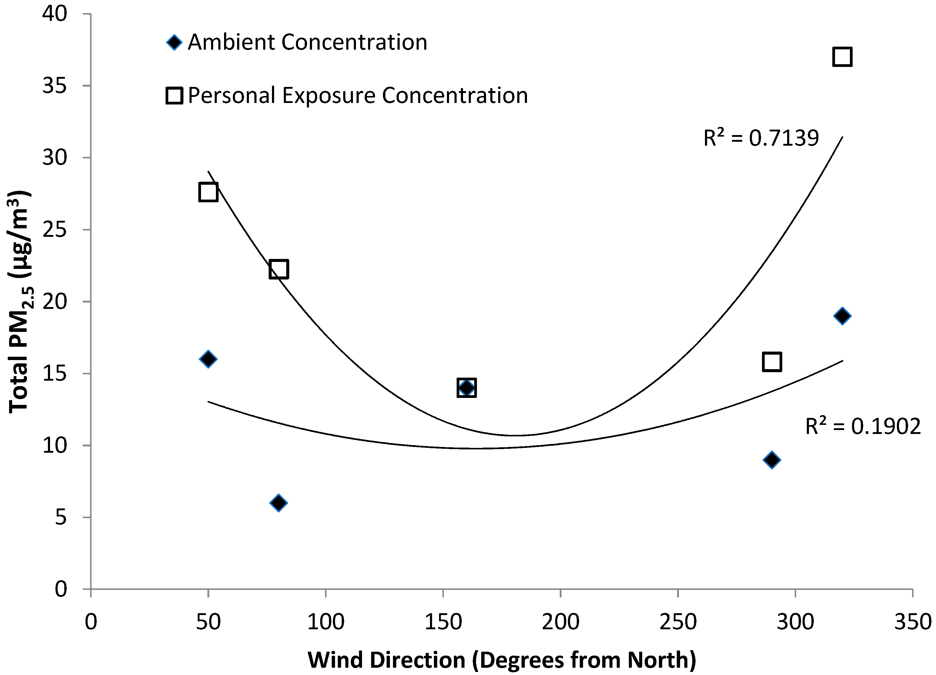
13]. One of the most interesting correlations found in this analysis was between wind direction and PM2.5 concentrations, with wind blowing from southerly directions significantly increasing personal exposure to PM2.5 along the bicycle path. It is not possible in this study to delineate the influence of the Macdonald-Cartier Freeway (highway 401), which is one of the busiest highway in North America and located immediately south of the study area, from the more regional distribution of major polluters including the many coal power plants located south in the Midwestern United States; however, literature exists supporting the latter [20]. The effect is much more pronounced with personal exposure measurements than with ambient concentrations, suggesting that ambient monitors underestimate the magnitude of the influence of wind direction. One policy that may be employed to mitigate this discrepancy would be to issue a warning on days with high ambient pollution and wind from the south for vulnerable populations considering outdoor physical activity.
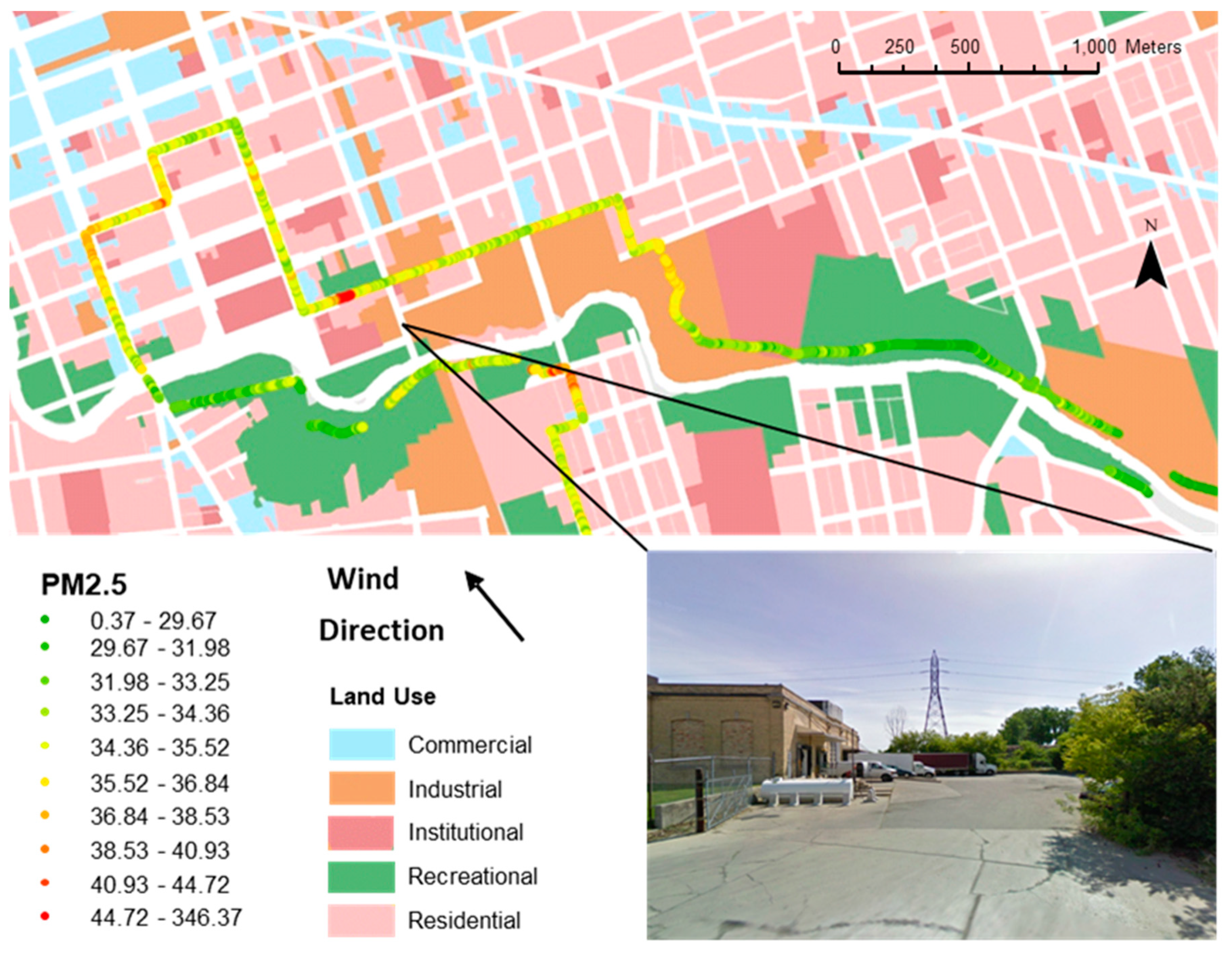
4.2. Hotspots

Previous research concluded that PM2.5 hotspots are chance occurrences [13]; however, our study has found consistency between days in several geographic locations. Specifically, hotspots were found in four areas: the busiest bridge in London, the downtown urban core, and two sites which were undergoing road construction during the week of the study. Traffic is known to influence PM2.5 but it is not known what, if any, additional factors a bridge may have over a land intersection with similar traffic volume. It does suggest that there is merit in separate bicycle bridges which exist in London, Ontario, but were unfortunately not part of this study. The second major hotspot is the urban core, which is also the site of high traffic levels and a high concentration of non-residential activities. It is also possible that an “urban canyon effect” is present, whereby generally poor airflow due to the higher density of buildings may be partly causing pollutants to be trapped at street level; however, this is normally a phenomenon observed in much more highly developed cities such as Hong Kong [23]. Finally, previous research found similar results for construction sites and personal exposure to PM10 [11]. A simple policy suggestion that can minimize exposure to PM2.5 for cyclists who are concerned about air pollution (i.e., elderly or asthmatics) would be to use signage to temporarily detour bicycle routes around the vicinity of construction sites.

4.3. Correlation between Elements of the Environment and Personal Exposure to PM2.5

Many elements of the built environment were significantly correlated with PM2.5 exposure across all study days; however, most showed mixed positive and negative relationships. The mixed correlation found between concentrations of PM2.5 and the road type (pathway or on road) and between the regions of high concentrations and low concentrations is not in agreement with previous research with cyclist commuters which found significantly greater exposure levels of both benzene and general particulate matter for those who traveled by road compared to path [41]. It is thus possible that PM2.5 is less influenced by the cyclists’ position relative to traffic at very short distances compared to other air pollutants. This is also evident in the mixed correlations with both bus and truck routes. Bus routes possibly due to London’s public transit authority incorporating hybrid electric buses into the fleet which may have reduced PM2.5 concentrations around the cyclists. A statistically higher portion of the cycled network in the 20% highest PM2.5 concentration category was designated as truck routes compared to the remainder of the cycled network on two of the three days. This suggests the possibility that single events, such as a cyclist following a truck, may significantly influence personal exposure to PM2.5. However, as these do not occur consistently, there is low merit avoiding these roads designated for either bus or truck based upon PM2.5 measurements in this study.
Traffic has been cited in the literature as a determinant of PM2.5 exposure; however, this relationship is far from conclusively established. For example, Thai, McKendry and Brauer [11] found little influence of traffic on PM2.5 personal exposure to cyclists but did find a relationship with ultrafine particles. Our research supports the connection, with several predictors for traffic in our study being significantly correlated with personal exposure to PM2.5. Furthermore, correlations were consistently higher in the regions with the highest pollution concentrations using both traffic count and traffic density measures. Traffic density was one of the strongest overall determinants for PM2.5, doubling the correlation found with traffic counts. This emphasizes the importance of spatial considerations, as air pollution dispersion is not confined to street segments. The negative correlation between PM2.5 and variables such as the distance to nearest 400 series highway, arterial roads, intersection, traffic Light, and stop sign on most study days suggests a strong influence of traffic, especially areas where traffic accelerates and decelerates. Specifically, the lower distance to arterials and to traffic lights in the regions with the highest pollution on all days suggests the particular importance of these two factors when planning future bike routes or route designations. Road surface area was also strongly correlated to personal exposure to fine particulate matter, especially on days with higher ambient PM2.5. This possibly reflects the phenomena of slower traffic resulting from the increased area for vehicles, compounding the emissions by having more accelerations and decelerations. Planners of future bicycle paths or designations should, therefore, whenever possible, avoid sources where traffic accelerates and decelerates, especially minimizing the distance to the nearest traffic light, which was the strongest predictor variable. Furthermore, cycling routes should be segregated, if possible, 100 m from arterial roads, and avoid commercial and industrial sites.
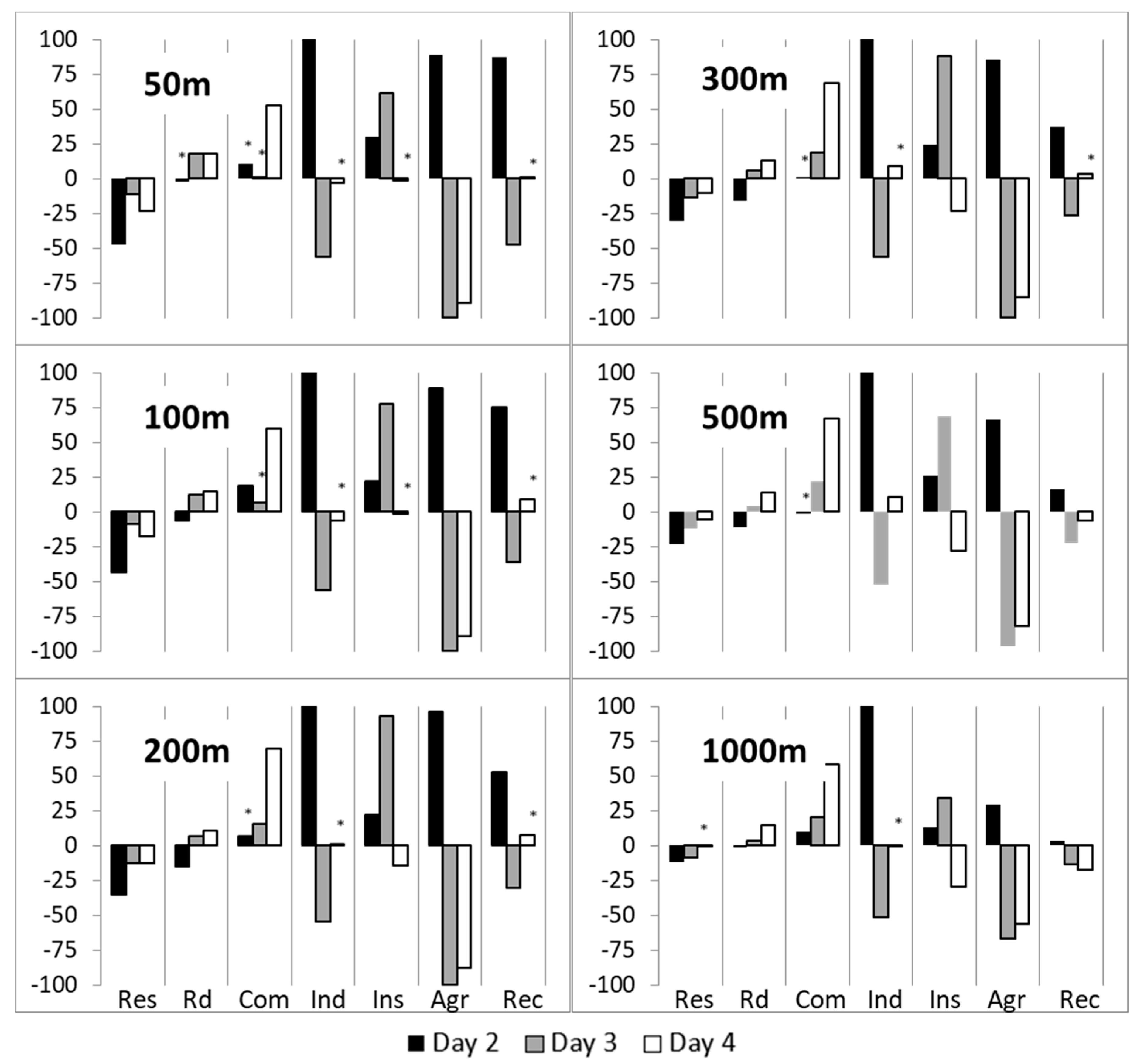
The negative correlation between the number of street trees located within 25 m of the path with personal exposure to PM2.5 and the evidence that route segments which contain more street trees are also those with the lowest air pollution concentration suggest an important role for street trees in minimizing exposure. The relationship was most profound on the days with the highest ambient measurements, day 3 and 4, signifying that trees may play an especially important role in reducing street-level PM2.5 during days that exceed the provincial health guidelines for healthy activity. The similar trend in recreational land use on days with higher pollution levels further supports this conclusion. It should be cautioned that it is not known whether trees reduce PM2.5 concentrations for cyclists, or if trees are preferentially planted (or are more likely to survive) in microenvironments with low PM2.5.
Other land use determinants for air pollution are generally mixed in their effect. The low fine particulate matter correlation and concentration in areas with high residential zoning, especially on days with low ambient pollution concentration, indicate that PM2.5 sources from the home such as cooking or smoking generally do not have a major influence on personal exposure to cyclists. It is also highly probable that the presence of residential zoning infers the absence of another potentially higher polluting land use. The correlation between commercial zoning and high PM2.5 concentrations on days with moderate and high ambient levels signifies that commercial activity has a role in the generation of PM2.5. This conclusion is strengthened by the similar pattern found with development density. PM2.5 concentrations were positively correlated to industrial land use area except on the day with the highest ambient PM2.5 concentration, where the influence was lower. This is possibly due to regional forces washing out the influence of local industrial PM2.5 sources. Institutional and agricultural land uses appeared to have a mixed and weak influence on PM2.5 concentrations possibly due to the generally low occurrences of these land uses along bicycle paths. Similarly, land use mix and speed limits were two predictor variables that showed mixed relationships with PM2.5 concentration with no apparent trend. To sum: bicycle routes should, if possible, travel through residential and recreational land uses avoiding traffic lights and arterial roads. Industrial sites should be avoided on low pollution days, and nearby street trees may reduce personal exposure to air pollution.
Caution must be exercised when interpreting these results, as determinants of air pollution are often linked with the interactions between them still not well understood. The correlation portion of this analysis assumed a linear relationship between elements of the environment and exposure to PM2.5, which, despite being a traditional statistical analysis, may not reflect reality. For example, increased road surface area could amplify PM2.5 release creating an exponential relationship from feedback caused by decreased speed due to increased traffic, or street trees may only influence PM2.5 concentrations when they reach a critical density. The high variability between days in the linear regression model suggests that elements of the natural environment must be incorporated into a final model, which was unfortunately not possible in this analysis due to the low number of sample days. The analysis comparing the regions with the highest 20% to the lowest 80% PM2.5 concentrations was highly susceptible to unpredictable variations in traffic, such as the cyclist following a bus or truck, and construction; however, our multi-day analysis helps minimize this concern. These data must be interpreted with caution because our measures for wind speed (and direction) were taken at one station in the city rather than the exact same location where personal PM2.5 exposure measures were recorded.

4.4. Implications for Public Health and Policy

Our research has found many incidences of personal exposure to PM2.5 exceeding the Ontario Ministry of Environment’s guidelines for healthy activity. Mitigation strategies aimed at balancing the health benefits of cycling with the environmental exposure to pollutants can take on two forms: behavioural modification and infrastructure modification. This research has provided evidence supporting both efforts. Infrastructure changes are limited by the need to connect people to where they want to go, thus planning decisions are constrained to elements amenable to change. Cycle paths can be created or designated to minimize pollution exposure using models which consider the environmental factors that were revealed here to be correlated with personal exposure to PM2.5, and are found in the zones with the highest observed concentrations. Alternative routes may also be made available to vulnerable populations to minimize exposure. A linear regression model which incorporates both elements of the natural and built environment can be used for planning future routes though it should be field tested in the new locale to ensure transferability. Although we have shown here that pollution concentration varies significantly between and within routes, the question remains as to the medical relevance of this difference; i.e., how exposure to different pollution concentrations can differentially damage one’s health. This study has employed novel tools including combining a high resolution personal monitor with a portable GPS device, and outlined methodologies for incorporating factors of the natural and built environment into a greater understanding of pollution exposure during the cycling adults. This research ultimately supports the important role of commuter agency and planning in the creation of healthy microenvironments. Future research should combine this novel instrumentation and spatial analysis techniques with health outcomes to provide a link which can be used to strengthen mitigation strategies. This case study should be repeated using different technical specifications (e.g., route selection, survey timing, proximity defined by different buffer sizes and types, etc.) and by applying different spatial and non-spatial modeling approaches.

Author Contributions

Conceptualization, J.G., M.M., X.X., and I.L.; methodology, J.G., M.M., X.X., and I.L.; software, M.M.; validation, M.M.; formal analysis, J.G. and M.M.; investigation, J.G. and M.M.; resources, J.G., M.M., X.X. and I.L.; data curation, M.M.; writing—original draft preparation, J.G. and M.M.; writing—review and editing, J.G., M.M., X.X., I.L. and T.S.; visualization, M.M. and T.S.; supervision, J.G.; project administration, J.G.; funding acquisition, J.G.

Funding

This project received funding from the Children’s Health Foundation through trainee support programs of the Children’s Health Research Institute.

Acknowledgments

Thanks to Eric Simard, Richard Sadler, Don Lafreniere, Alex Mates, and Martin Healy for fieldwork assistance, and Sandra Kulon for GIS support.

Conflicts of Interest

The authors declare no conflict of interest.

Appendix A

Bootstrapping results for linear regression model: Bootstrapping provides an alternative to estimates when parametric assumptions in are in doubt. Specifically, the assumption of independent sampling is broken as the data points are necessarily spatially autocorrelated. Bootstrapping reveals more accurate significance values present in the regression model by using new standard error values and confidence intervals based upon multiple (in this case 1000) re-sampling iterations within the sample. Included are examples of the bootstrap output from SPSS 19 (IBM) used in this paper.
Table A1. Day2. Bootstrap for Coefficients.
ModelBBiasSESig. (2-Tailed)95% CI (L)95% CI (U)
(Constant)15.7510.0040.8740.00114.31217.703
PathType−2.0050.0020.250.001−2.452−1.469
SpeedLM−0.01−6.55 × 10−50.0080.202−0.0260.008
Traffic0.1043.48 × 10−50.0110.0010.0820.125
TruckRout3.5620.0020.4510.0012.6014.411
BusRout−2.4370.0010.1580.001−2.752−2.117
Dist4000−2.36 × 10−73.11 × 10−50.00100
DistArt0.0017.51 × 10−700.0010.0010.002
DistInt0.0081.65 × 10−50.0010.0010.0070.01
Res100 m−0.0552.31 × 10−70.0030.001−0.061−0.049
Road300 m−0.02100.0150.17−0.050.011
Ind300 m0.11400.0060.0010.1040.126
Agr200 m0.006−5.21 × 10−50.0140.648−0.0260.031
Rec100 m−0.056−8.96 × 10−60.0050.001−0.066−0.047
LUM500 m10.753−0.0091.0120.0018.44712.314
DD300 m−16.236−0.0110.8090.001−17.908−14.793
Table A2. Day3: Bootstrap for Coefficients.
ModelBBiasStd. ErrorSig. (2-Tailed)95% CI (L)95% CI (U)
(Constant)30.143−0.0220.3220.00129.53630.798
PathType5.734−0.0030.2930.0015.1386.311
Speed−0.0426.17 × 10−50.0040.001−0.05−0.035
TrafficDEns0.0621.53 × 10−50.0020.0010.0580.067
Truck−3.047−0.0010.2260.001−3.504−2.579
Bus−1.54−0.0070.110.001−1.756−1.334
DistInt−0.0064.24 × 10−50.0010.001−0.007−0.005
DistArt0.0053.70 × 10−600.0010.0040.005
Trees−0.11300.0050.001−0.124−0.103
Res100 m−0.00400.0020.054−0.0081.51 × 10−5
Com1000 m−0.05100.0160.003−0.084−0.022
Road50 m0.03100.010.0050.0110.051
Ind1000 m−0.13200.0060.001−0.145−0.119
Inst300 m0.04700.0050.0010.0380.057
Agr500 m−0.1300.0050.001−0.141−0.12
Rec50 m−0.0244.10 × 10−60.0040.001−0.032−0.017
LUM50 m4.3370.030.4870.0013.435.343
DD500 m1.2090.0051.1470.306−0.9343.563
Table A3. Day4: Bootstrap for Coefficients.
ModelBBiasStd. ErrorSig. (2-Tailed)95% CI (L)95% CI (U)
(Constant)33.35−0.0020.2440.00132.87833.82
PathyType2.487−0.0010.1140.0012.2692.712
Speed−0.0732.56 × 10−50.0030.001−0.078−0.067
TrafDens0.0158.95 × 10−60.0010.0010.0130.017
Truck1.911−0.0050.1160.0011.6722.132
Bus−1.676−0.0020.0590.001−1.796−1.565
Trees−0.061−5.42 × 10−50.0040.001−0.069−0.054
Dist400−0.001−1.43 × 10−71.13 × 10−50.001−0.0010
DistArt−0.0021.56 × 10−800.001−0.003−0.002
DistTlight−0.0021.32 × 10−600.001−0.002−0.002
Res1000 m−0.005−6.23 × 10−50.0040.208−0.0130.003
Com1000 m0.02700.010.0050.0090.046
Road1000 m0.5770.0020.0390.0010.5020.655
Ind500 m0.05300.0050.0010.0440.062
Inst1000 m−0.049−3.68 × 10−60.0030.001−0.055−0.043
Rec1000 m−0.131−5.74 × 10−50.0040.001−0.139−0.123
LUM300 m−3.4277.82 × 10−60.2560.001−3.954−2.954
DD1000 m−10.98−0.0721.4210.001−13.8−8.311

References

  1. Pucher, J.; Buehler, R. Why Canadians cycle more than Americans: A comparative analysis of bicycling trends and policies. Transp. Policy 2006, 13, 265–279. [Google Scholar] [CrossRef] [Green Version]
  2. Pucher, J.; Buehler, R.; Seinen, M. Bicycling renaissance in North America? An update and re-appraisal of cycling trends and policies. Transp. Res. Part A Policy Pract. 2011, 45, 451–475. [Google Scholar] [CrossRef]
  3. Rojas-Rueda, D.; de Nazelle, A.; Tainio, M.; Nieuwenhuijsen, M.J. The health risks and benefits of cycling in urban environments compared with car use: Health impact assessment study. BMJ 2011, 343. [Google Scholar] [CrossRef] [PubMed]
  4. Avila-Palencia, I.; de Nazelle, A.; Cole-Hunter, T.; Donaire-Gonzalez, D.; Jerrett, M.; Rodriguez, D.A.; Nieuwenhuijsen, M.J. The relationship between bicycle commuting and perceived stress: A cross-sectional study. BMJ Open 2017, 7. [Google Scholar] [CrossRef] [PubMed]
  5. Flint, E.; Cummins, S.; Sacker, A. Associations between active commuting, body fat, and body mass index: Population based, cross sectional study in the United Kingdom. BMJ 2014, 349. [Google Scholar] [CrossRef] [PubMed]
  6. Boogaard, H.; Borgman, F.; Kamminga, J.; Hoek, G. Exposure to ultrafine and fine particles and noise during cycling and driving in 11 Dutch cities. Atmos. Environ. 2009, 43, 4234–4242. [Google Scholar] [CrossRef]
  7. Kendrick, C.M.; Moore, A.; Haire, A.; Bigazzi, A.; Figliozzi, M.; Monsere, C.M.; George, L. Impact of Bicycle Lane Characteristics on Exposure of Bicyclists to Traffic-Related Particulate Matter. Transp. Res. Rec. 2011, 2247, 24–32. [Google Scholar] [CrossRef]
  8. Sofowote, U.M.; Healy, R.M.; Su, Y.; Debosz, J.; Noble, M.; Munoz, A.; Jeong, C.H.; Wang, J.M.; Hilker, N.; Evans, G.J.; et al. Understanding the PM2.5 imbalance between a far and near-road location: Results of high temporal frequency source apportionment and parameterization of black carbon. Atmos. Environ. 2018, 173, 277–288. [Google Scholar] [CrossRef]
  9. Wilson, J.G.; Kingham, S.; Pearce, J.; Sturman, A.P. A review of intraurban variations in particulate air pollution: Implications for epidemiological research. Atmos. Environ. 2005, 39, 6444–6462. [Google Scholar] [CrossRef]
  10. McNabola, A.; Broderick, B.M.; Gill, L.W. Relative exposure to fine particulate matter and VOCs between transport microenvironments in Dublin: Personal exposure and uptake. Atmos. Environ. 2008, 42, 6496–6512. [Google Scholar] [CrossRef]
  11. Thai, A.; McKendry, I.; Brauer, M. Particulate matter exposure along designated bicycle routes in Vancouver, British Columbia. Sci. Total Environ. 2008, 405, 26–35. [Google Scholar] [CrossRef] [PubMed]
  12. Kaur, S.; Nieuwenhuijsen, M.J.; Colvile, R.N. Fine particulate matter and carbon monoxide exposure concentrations in urban street transport microenvironments. Atmos. Environ. 2007, 41, 4781–4810. [Google Scholar] [CrossRef]
  13. Greaves, S.; Issarayangyun, T.; Liu, Q. Exploring variability in pedestrian exposure to fine particulates (PM2.5) along a busy road. Atmos. Environ. 2008, 42, 1665–1676. [Google Scholar] [CrossRef]
  14. Bevan, M.A.J.; Proctor, C.J.; Baker-Rogers, J.; Warren, N.D. Exposure to carbon monoxide, respirable suspended particulates and volatile organic compounds while commuting by bicycle. Environ. Sci. Technol. 1991, 25, 788–791. [Google Scholar] [CrossRef]
  15. Charron, A.; Harrison, R.M. Fine (PM2.5) and Coarse (PM2.5-10) Particulate Matter on A Heavily Trafficked London Highway: Sources and Processes. Environ. Sci. Technol. 2005, 39, 7768–7776. [Google Scholar] [CrossRef] [PubMed]
  16. Adams, H.S.; Nieuwenhuijsen, M.J.; Colvile, R.N.; McMullen, M.A.S.; Khandelwal, P. Fine particle (PM2.5) personal exposure levels in transport microenvironments, London, UK. Sci. Total Environ. 2001, 279, 29–44. [Google Scholar] [CrossRef]
  17. Hoek, G.; Beelen, R.; de Hoogh, K.; Vienneau, D.; Gulliver, J.; Fischer, P.; Briggs, D. A review of land-use regression models to assess spatial variation of outdoor air pollution. Atmos. Environ. 2008, 42, 7561–7578. [Google Scholar] [CrossRef]
  18. Goswami, E.; Larson, T.; Lumley, T.; Liu, L.-J.S. Spatial characteristics of fine particulate matter: Identifying representative monitoring locations in Seattle, Washington. J. Air Waste Manag. Assoc. 2002, 52, 324–333. [Google Scholar] [CrossRef] [PubMed]
  19. Martuzevicius, D.; Grinshpun, S.A.; Reponen, T.; Górny, R.L.; Shukla, R.; Lockey, J.; Hu, S.; McDonald, R.; Biswas, P.; Kliucininkas, L.; et al. Spatial and temporal variations of PM2.5 concentration and composition throughout an urban area with high freeway density—The Greater Cincinnati study. Atmos. Environ. 2004, 38, 1091–1105. [Google Scholar] [CrossRef]
  20. Lee, P.K.H.; Brook, J.R.; Dabek-Zlotorzynska, E.; Mabury, S.A. Identification of the Major Sources Contributing to PM2.5 Observed in Toronto. Environ. Sci. Technol. 2003, 37, 4831–4840. [Google Scholar] [CrossRef]
  21. Smargiassi, A.; Baldwin, M.; Pilger, C.; Dugandzic, R.; Brauer, M. Small-scale spatial variability of particle concentrations and traffic levels in Montreal: A pilot study. Sci. Total Environ. 2005, 338, 243–251. [Google Scholar] [CrossRef]
  22. Berghmans, P.; Bleux, N.; Panis, L.I.; Mishra, V.K.; Torfs, R.; Van Poppel, M. Exposure assessment of a cyclist to PM10 and ultrafine particles. Sci. Total Environ. 2009, 407, 1286–1298. [Google Scholar] [CrossRef] [PubMed]
  23. Chan, L.Y.; Kwok, W.S.; Lee, S.C.; Chan, C.Y. Spatial variation of mass concentration of roadside suspended particulate matter in metropolitan Hong Kong. Atmos. Environ. 2001, 35, 3167–3176. [Google Scholar] [CrossRef]
  24. Briggs, D.J.; de Hoogh, K.; Morris, C.; Gulliver, J. Effects of travel mode on exposures to particulate air pollution. Environ. Int. 2008, 34, 12–22. [Google Scholar] [CrossRef] [PubMed]
  25. Bigazzi, A.Y.; Figliozzi, M.A. Review of Urban Bicyclists’ Intake and Uptake of Traffic-Related Air Pollution. Transp. Rev. 2014, 34, 221–245. [Google Scholar] [CrossRef]
  26. Statcan. Census Profile, 2016 Census: London [Population Centre], Ontario and Ontario [Province]. Available online: http://www12.statcan.gc.ca/census-recensement/2016/dp-pd/prof/index.cfm?Lang=E (accessed on 8 August 2018).
  27. Avery, C.L.; Mills, K.T.; Williams, R.; McGraw, K.A.; Poole, C.; Smith, R.L.; Whitsel, E.A. Estimating error in using ambient PM2.5 concentrations as proxies for personal exposures: A review. Epidemiology 2010, 21, 215–223. [Google Scholar] [CrossRef]
  28. Bowker, G.E.; Baldauf, R.; Isakov, V.; Khlystov, A.; Petersen, W. The effects of roadside structures on the transport and dispersion of ultrafine particles from highways. Atmos. Environ. 2007, 41, 8128–8139. [Google Scholar] [CrossRef] [Green Version]
  29. Roorda-Knape, M.C.; Janssen, N.A.H.; De Hartog, J.J.; Van Vliet, P.H.N.; Harssema, H.; Brunekreef, B. Air pollution from traffic in city districts near major motorways. Atmos. Environ. 1998, 32, 1921–1930. [Google Scholar] [CrossRef]
  30. DeGaetano, A.T.; Doherty, O.M. Temporal, spatial and meteorological variations in hourly PM2.5 concentration extremes in New York City. Atmos. Environ. 2004, 38, 1547–1558. [Google Scholar] [CrossRef]
  31. Xie, Z.; Yan, J. Kernel Density Estimation of traffic accidents in a network space. Comput. Environ. Urban Syst. 2008, 32, 396–406. [Google Scholar] [CrossRef] [Green Version]
  32. Eeftens, M.; Beelen, R.; de Hoogh, K.; Bellander, T.; Cesaroni, G.; Cirach, M.; Declercq, C.; Dėdelė, A.; Dons, E.; de Nazelle, A.; et al. Development of Land Use Regression Models for PM2.5, PM2.5 Absorbance, PM10 and PMcoarse in 20 European Study Areas; Results of the ESCAPE Project. Environ. Sci. Technol. 2012, 46, 11195–11205. [Google Scholar] [CrossRef] [PubMed]
  33. Su, J.G.; Jerrett, M.; Beckerman, B. A distance-decay variable selection strategy for land use regression modeling of ambient air pollution exposures. Sci. Total Environ. 2009, 407, 3890–3898. [Google Scholar] [CrossRef] [PubMed]
  34. Larsen, K.; Gilliland, J.; Hess, P.; Tucker, P.; Irwin, J.; He, M. The Influence of the Physical Environment and Sociodemographic Characteristics on Children’s Mode of Travel to and From School. Am. J. Public Health 2009, 99, 520–526. [Google Scholar] [CrossRef]
  35. Tucker, P.; Irwin, J.D.; Gilliland, J.; He, M.; Larsen, K.; Hess, P. Environmental influences on physical activity levels in youth. Health Place 2009, 15, 357–363. [Google Scholar] [CrossRef] [PubMed]
  36. IBM. IBM SPSS Statistics for Windows; Version 19.0; IBM Corp.: Armonk, NY, USA, 2017. [Google Scholar]
  37. Wilks, D.S. Resampling Hypothesis Tests for Autocorrelated Fields. J. Clim. 1997, 10, 65–82. [Google Scholar] [CrossRef]
  38. Gauvin, S.; Reungoat, P.; Cassadou, S.; Déchenaux, J.; Momas, I.; Just, J.; Zmirou, D. Contribution of indoor and outdoor environments to PM2.5 personal exposure of children—VESTA study. Sci. Total Environ. 2002, 297, 175–181. [Google Scholar] [CrossRef]
  39. Yip, F.Y.; Keeler, G.J.; Dvonch, J.T.; Robins, T.G.; Parker, E.A.; Israel, B.A.; Brakefield-Caldwell, W. Personal exposures to particulate matter among children with asthma in Detroit, Michigan. Atmos. Environ. 2004, 38, 5227–5236. [Google Scholar] [CrossRef]
  40. Levene, H. Robust tests for equality of variances. In Contributions to Probability and Statistics Essays in Honor of Harold Hotelling; Stanford University Press: London, UK, 1961; pp. 279–292. [Google Scholar]
  41. Kingham, S.; Meaton, J.; Sheard, A.; Lawrenson, O. Assessment of exposure to traffic-related fumes during the journey to work. Transp. Res. Part D Transp. Environ. 1998, 3, 271–274. [Google Scholar] [CrossRef]
Figure 1. Process of assigning data points to line segments. Each spatially identified pollution concentration reading (red circle) within the search radius of 25 m (blue circle) is assigned to the nearest 1 m segment (black line) and the mean value was taken. Predictor variables are also assigned to each 1 m in similar fashion for statistical analysis.
Urbansci 02 00120 g001
Figure 2. Influence of wind direction on personal exposure measurements and ambient PM2.5. A second order polynomial regression line of best fit was added to both personal exposure and ambient measurements. Residuals were significantly different from observed values for the ambient measurements (ANOVA, p = 0.03) but not personal exposure concentrations (ANOVA, p = 0.83).
Urbansci 02 00120 g002
Figure 3. PM2.5 concentrations from a typical day labeled by decile. PM2.5 levels are generally distributed unevenly along the cycled routes, with the higher personal exposure concentrations in the urban core and lower concentrations extending out into the suburbs. All measurements in μg/m3.
Urbansci 02 00120 g003
Figure 4. PM2.5 concentrations from a typical day labeled using Ministry of the Environment’s air quality index (AQI) categories. Concentrations of PM2.5 are generally within the Moderate (23 to 45 μg/m3) category but several areas primarily in the urban core enter the Poor (46 to 90 μg/m3) category. Observations along portions of the route extending west that traveled through parks were in the Good (12 to 22 μg/m3) category. The intra-urban differences in PM2.5 exposure concentrations when using the AQI categories are less pronounced compared to using deciles, but more meaningful from a public health perspective.
Urbansci 02 00120 g004
Figure 5. Segment of a single route with 1-s resolution PM2.5 concentration measurements overlaid on a land use map. Correlation is apparent between personal exposure to PM2.5 and land use. The loading bay with idling vehicles and wind direction may account for the nearby peak in PM2.5. PM2.5 concentration in μg/m3.
Urbansci 02 00120 g005
Figure 6. Map of London, Ontario with the top 1% of all recorded values for each of the 5 study days. Clustering is apparent in three regions: approaching the bridge in the west part of the city (1); the downtown urban core (2); and two spots which were noted for being under construction during the course of the study (3, 4).
Urbansci 02 00120 g006
Figure 7. Map of London, Ontario highlighting very poor (PM2.5 > 91 μg/m3) pollution concentrations for each of the 5 study days. The very poor concentration category is determined by the Ontario Ministry of the Environment’s AQI. Clustering is more apparent when compared to the top 1% values (Figure 6); however, the same 4 hotspots are found, giving health relevance to these observations.
Urbansci 02 00120 g007
Figure 8. Linear regression models for three study days. Bootstrapping revealed several biases that were significant (see, Appendix A): speed limit, road 300 m, and agricultural 200 m on day 2 (Table A1); residential 100 m and development density 500 m on day 3 (Table A2); and residential 1000 m (Table A3).
Urbansci 02 00120 g008
Figure 9. Percent change in traffic-related predictor variables between the 20% most heavily polluted segments of the cycled network and the remainder of the cycled path. * denotes an insignificant difference (two-tailed t-test, equal variances not assumed p > 0.05).
Urbansci 02 00120 g009
Figure 10. Percent change in urban form related predictor variables between the 20% most heavily polluted segments of the cycled network and the remained of the cycled path.
Urbansci 02 00120 g010
Figure 11. Percent change in land use predictor variables at different buffer distances between the 20% most heavily polluted segments of the cycled network and the remainder of the cycled path. * denotes an insignificant difference (two-tailed t-test, equal variances not assumed p > 0.05). Res = Residential, Rd = Road, Com = Commercial, Ind = Industrial, Ins = Institutional, Agr = Agriculture, and Rec = Recreational.
Urbansci 02 00120 g011
Figure 12. Percent change in land use mix and development density predictor variables between the 20% most heavily polluted segments of the cycled network and the remainder of the cycled path.
Urbansci 02 00120 g012
Table 1. Land uses located within 100 m of the study route compared with the city designated bicycling network.
Land Use within 100 mTotal Network of City Bike RoutesStudy Routes
Agriculture3.3%1.0%
Commercial7.0%8.5%
Industrial6.3%4.2%
Recreation15.7%17.7%
Residential55.6%57.1%
Source: City of London.
Table 2. Measurements of consistency in PM2.5 concentration readings between units before and after experiment in μg/m3.
UnitPre-TestPostChange
12.733.470.74
22.305.923.63
33.550.59−2.96
42.261.09−1.17
54.25417.40413.15 *
* Unit 6 failed after day 4 of the study thus data from day 5 was discarded.
Table 3. Comparison between ambient PM2.5 and measured personal exposure to PM2.5.
Ambient μg/m3Bicycle Average μg/m3Unit 1 μg/m3Unit 2 μg/m3Unit 3 μg/m3Unit 4 μg/m3Unit 5 μg/m3
Day 1622x15312320
Day 2916131517259
Day 319373944293439
Day 416282632222929
Day 51414*17141312
Note: Average ambient concentrations obtained from the Ontario Ministry of the Environment’s London air pollution monitor using hourly measurements from 7 AM to 9 AM each day were less than or equal to the mean readings obtained from the cyclist’s personal monitoring device during the same time period. * Machine Error, x = participant error.
Table 4. Average meteorological conditions between 7 AM and 9 AM for the five study days.
DayTemperature (°C)Relative Humidity (%)Wind Direction (o)Wind Speed (km/h)
121.9748011
222.77029010
322.2733208
421.7705010
523.1681608
Data was obtained from the National Climate Data and Information Archive from Environment Canada (2010). Wind direction is given in degrees from geographic north.
Table 5. Traffic-related predictor variables analyzed using ANOVA and Pearson’s R for correlation to PM2.5 exposure.
Day 2Day 3Day 4
Path Type−0.2520.3170.050
Speed Limit−0.280.117−0.045
Traffic0.1340.0740.107
Traffic Density0.1230.1050.318
Truck Route0.272−0.0630.127
Bus Route−0.1810.060−0.061
Note: Bootstrapping revealed minimal bias in all cases (data not shown).
Table 6. Urban form related predictor variables for PM2.5 exposure analyzed using Pearson’s R.
Day 2Day 3Day 4
Distance to 400 series highway−0.107 *0.002−0.379 *
Distance to arterial road−0.206 *0.092 *−0.250 *
Distance to nearest intersection0.262 *−0.275 *−0.080 *
Distance to nearest traffic Light−0.027 *−0.018 *−0.257 *
Distance to nearest stop sign0.245 *−0.151 *−0.087 *
Street Trees−0.034 *−0.175 *−0.233 *
Note: Street trees are number found within a 25 m buffer. Bootstrapping found minimal bias (data not shown). * indicates a significant correlation with p < 0.05.
Table 7. Pearson’s R correlation between land use variables and personal PM2.5 concentrations.
ResidentialDay 2Day 3Day 4CommercialDay 2Day 3Day 4
50 m−0.3160.101−0.09950 m0.002 *0.0830.138
100 m−0.3270.127−0.092100 m0.017 *0.0750.162
200 m−0.3120.106−0.099200 m0.001 *0.0770.195
300 m−0.3020.089−0.109300 m−0.007 *0.0780.211
500 m−0.2740.0670.176500 m−0.016 *0.0720.225
1000 m−0.2010.027−0.371000 m−0.017 *0.1020.320
Road Industrial
50 m−0.0810.2410.14350 m0.211−0.0430.075
100 m−0.1250.2390.127100 m0.235−0.0390.091
200 m−0.2300.2280.143200 m0.270−0.0550.124
300 m−0.2420.2170.155300 m0.280−0.0870.158
500 m−0.2020.1940.176500 m0.274−0.1170.187
1000 m−0.1020.1500.2631000 m0.178−0.1720.167
Institutional Agricultural
50 m0.010 *0.0520.018 *50 m0.084−0.073−0.040
100 m0.008 *0.0790.002 *100 m0.084−0.073−0.040
200 m0.013 *0.115−0.033200 m0.089−0.075−0.022
300 m0.0220.115−0.055300 m0.086−0.074−0.011 *
500 m0.0350.102−0.069500 m0.078−0.081−0.07 *
1000 m0.0200.061−0.1041000 m0.029−0.0550.029
Recreational
50 m0.217−0.297−0.056
100 m0.221−0.278−0.056
200 m0.205−0.285−0.073
300 m0.189−0.283−0.079
500 m0.163−0.283−0.136
1000 m0.172−0.230−0.324
Notes: Percent of space within buffers sized 50 m to 1000 m occupied by a land use. Bold values represent the buffer size with the greatest correlation above 0.05 which was employed in the linear model creation. Bootstrapping found minimal bias (data not shown). * indicates insignificant correlation with p < 0.05.
Table 8. Pearson’s R correlation between land use mix and development density and personal exposure to PM2.5 concentrations.
Land Use Mix Development Density
Day 2Day 3Day 4Day 2Day 3Day 4
50 m−0.0200.2150.10450 m−0.2780.1580.130
100 m0.0690.1490.129100 m−0.2690.1850.152
200 m0.0370.0830.102200 m−0.2720.1920.138
300 m0.176−0.0510.159300 m−0.2870.2040.149
500 m0.240−0.1330.123500 m−0.2520.2200.189
1000 m0.212−0.01220.1201000 m−0.1870.1990.269
Note: All correlations were significant with p < 0.05 and bootstrapping found minimal. bias (data not shown).

