Abstract
Estimation of origin–destination (OD) demand plays a key role in successful transportation studies. In this paper, we consider the estimation of time-varying day-to-day OD flows given data on traffic volumes in a transportation network for a sequence of days. We propose a dynamic linear model (DLM) in order to represent the stochastic evolution of OD flows over time. DLMs are Bayesian state-space models which can capture non-stationarity. We take into account the hierarchical relationships between the distribution of OD flows among routes and the assignment of traffic volumes on links. Route choice probabilities are obtained through a utility model based on past route costs. We propose a Markov chain Monte Carlo algorithm, which integrates Gibbs sampling and a forward filtering backward sampling technique, in order to approximate the joint posterior distribution of mean OD flows and parameters of the route choice model. Our approach can be applied to congested networks and in the case when data are available on only a subset of links. We illustrate the application of our approach through simulated experiments on a test network from the literature.
1. Introduction
Given a geographic region, one of the main problems in planning and operating transportation systems is the estimation of origin–destination (OD) flows, i.e., the amount of trips made by people or freight between points in the region over a defined time interval. This is also referred to in the literature as the OD matrix estimation problem, since many initial models represented the vector of OD flows as a matrix.
OD flows are traditionally estimated through surveys, in which households or drivers are inquired about their daily journeys [1]. However, direct surveys are expensive and, due to this reason, they are in general carried out every decade [2]. This low frequency implies that planners may remain many years with no data on the evolution of OD flows over time.
In recent years, governments in urban regions have built traffic control systems in order to manage traffic congestion in transportation networks. Those systems automatically gather large amounts of data on traffic volumes at low cost on a daily or even hourly basis. This allowed in theory the indirect estimation of OD flows by means of mathematical models. The idea is that we can extract information on OD flows from data on traffic volumes if we have a suitable mathematical model which describes their relationships. Thus, OD matrix estimation from traffic volumes may be regarded as the inverse traffic assignment problem [2]. Within the traditional 4-step model, the traffic assignment problem corresponds to the final step, i.e., to the assignment of trips to a network after determination of generated and attracted trips per geographic region, their distribution among regions and their modal split [1]. The output of the traffic assignment step are predicted traffic volumes on links of a transportation network. OD matrix estimation from traffic volumes aims at estimating or reconstructing the trips that generated observed traffic volumes.
The early models for estimation of OD flows assumed that the transportation network from which one observes traffic volumes is not congested. We can trace back the first attempts to the work of Robillard [3], who applied linear regression to estimate OD flows from traffic volumes. Nguyen [4] proposed a model based on Beckman’s optimization model [5] for traffic assignment, whose solution is an estimate of the OD flows.
Van Zuylen and Willumsen [6] proposed a nonlinear programming model based on entropy maximization in which the constraints are the linear enconservation flow equations, whose solution corresponds to a maximum entropy OD flow configuration. Cascetta [7] proposed a generalized least squares (GLS) model which can cope with errors in observed traffic volumes by minimizing the Mahalanobis distance between predicted volumes and observed volumes. Cascetta and Nguyen [8] and Brenninger-Göthe and Jörnsten [9] proposed general frameworks which generalize previous models.
Fisk [10,11] proposed models which take into account traffic congestion, by seeking solutions which correspond to an equilibrium state as defined for example by Wardrop’s first principle [12,13]. Yang et al. [14] proposed a framework based on bilevel optimization, in which the first level corresponds to an objective function (e.g., maxent or GLS) subject to constraints which are obtained as a solution of a traffic assignment model in the second level. Due to the non-convex nature of the model, the authors proposed a heuristic procedure to solve it [15].
Cascetta and Postorino [16] formulated the OD matrix estimation problem as a compound fixed point problem, in which the solution of an inner fixed point problem corresponds to an equilibrium traffic assignment of an OD matrix obtained as a solution of an outer fixed point problem. In order to solve the problem, they propose a fixed point iteration based on the method of successive averages [17].
A common caveat in the abovementioned models is that they do not take variability of OD flows into account. Assuming that OD flows follow independent Poisson probability distributions, Vardi [18] considered the estimation of mean OD flows given a sample of observed traffic volumes’ vectors. Since the mean and variance of Poisson random variables are equal, variance of traffic volumes carry information on mean OD flows. He also assumed the existence of a single route for each OD pair, and proposed maximum likelihood and moment-based estimators for the mean OD flows.
Following Vardi’s work, Tebaldi and West [19] proposed Bayesian estimators for the case when a sample of size one is available for the traffic volumes vector. In some applications, it may be the case that a prior OD matrix may be available from older studies. A Bayesian statistical model allows the incorporation of knowledge on OD flows as a prior probability distribution, thereby improving modeling and inference. Hazelton [20,21,22] extended both Vardi’s and Tebaldi and West’s works. For example, both latter works assumed a single route in each OD pair, which is not realistic, while Hazelton considered multiple routes. In addition, the Poisson assumption poses computational hurdles for the application of Vardi’s or Tebaldi and West’s models to large-scale networks. The Hazelton solution was to approximate the distribution of OD flows with a multivariate normal density, which has more tractable computational properties, further assuming that the variances of OD flows are functions of their means as in the Poisson probability function.
More recent approaches consider the development of dynamic models for the estimation of OD flows. As traffic volumes are observed over time, we cannot ignore their temporal nature. Here, we must make a distinction between within-day and day-to-day dynamics. When considering within-day dynamics, one is concerned with the estimation of OD flows over the course of a single day [23,24,25]. In contrast, in day-to-day dynamics, we consider the estimation of time-varying OD flows for a reference time period, e.g., the morning peak, given a time series of observed traffic volumes over many consecutive days. It is assumed that this reference time period is long enough so that most trips in the study region start and finish within the observation period.
Hazelton [26] developed one of the first models for the estimation of day-to-day dynamic OD flows. The author assumes that mean OD flows are functions of parameters that do not change over time. Particular cases include constant demand, linear trend and weekday-weekend models. Parry and Hazelton [27] proposed a general Bayesian framework for the estimation of parameters of day-to-day dynamic traffic models. They assumed that OD flows vary according to a Markovian transition kernel, and proposed a Markov chain Monte Carlo (MCMC) algorithm for the estimation of parameters. Hazelton and Parry [28] proposed statistical methods to compare alternative day-to-day dynamic models.
A central aspect in the development of realistic day-to-day dynamic models is the modeling of users’ behavior through route choice models. In practice, users choose routes based on the travel times they have experienced over past days. Thus, a suitable route choice model should take into account the influence of past route costs on the decision of users in a given time. Watling and Cantarella [29,30] discuss models for the analysis of dynamic users’ behavior.
In this paper, we represent stochastic day-to-day OD flows as a dynamic linear model (DLM), which allows us to capture the time dependencies of OD flows as well as non-stationarity. In the formulation of the DLM, we take into account the variability originating from OD flows, user’s route choices and measurement of traffic volumes on links. The main contribution of our proposed model is that we represent route choices through a utility model which takes into account the adaptive behavior of users to experienced past route costs. This allows us to jointly estimate dynamic assignment matrices and OD flows in a statistically principled manner. In addition, our model does not rely on equilibrium assumptions, so that it can be equally applied to noncongested and congested networks. We also propose an MCMC algorithm, based on Gibbs sampling and forward filtering backward sampling, in order to approximate the joint posterior distributions of mean OD flows and parameters of the route choice model. We illustrate its application through numerical studies in a network from the literature.
This paper is organized as follows: in Section 2.1, we describe the proposed dynamic linear model; in Section 2.2, we describe a route choice model and an MCMC algorithm for the approximation of the joint posterior of mean OD flows and route choice parameters; in Section 3, we present numerical studies and discuss the results; finally, in Section 4, we draw some conclusions and propose further developments.
2. Modeling Framework
2.1. A Dynamic Linear Model for Day-to-Day OD Flows
In Section 2.1.1, we define the proposed dynamic linear model and in Section 2.1.2 we describe the procedure for estimating mean OD flows. A nomenclature with all symbols used may be found after the Conclusions section.
2.1.1. Model Definition
Dynamic linear models are defined by a state transition equation, which describes how a system evolves in time, and an observational equation, which describes how observed quantities relate to the system’s states. They have a Markovian structure and assume multivariate normal probability distributions for the random variables. System’s states are regarded as unobserved parameters whose estimation is done through Bayesian updating. We refer to [31] for an excellent introduction to the corresponding theory.
Let be a transportation network in which is a set of nodes, a set of directed links and a set of OD pairs. For a sequence of subsequent time periods , we define as the mean OD flow vector, in which is the mean OD flow for OD pair at time t and . We define as the vector of observed traffic volumes in a subset of links in a network at time t, in which is the observed volume on link and .
We consider the vector of mean OD flows as the unobserved system state vector, which depends only on its previous state at time plus a stochastic error. The vector of observed link volumes at time t depends only on the current unobserved vector of states, such that
We refer to Equation (1) as the dynamic model, while Equation (2) is the observational model. is the system matrix and is a stochastic error, where the letter “N” stands for the multivariate normal density with the appropriate dimension and is a covariance matrix also referred to as an evolution matrix. It governs the stochastic evolution of the system through time. We notice that . is an assignment matrix which relates mean OD flows to observed traffic volumes, while is a zero-mean error term which corresponds to the deviation of observed volumes relative to the expected value . We have that .
In order to fully determine the model given by Equations (1) and (2), we must specify the corresponding matrices. Regarding the system matrix, we assume that, in the short term, mean OD flows are locally constant. This implies that at time t mean OD flows should be approximately equal to mean OD flows at time , so that and , the identity matrix with the appropriate dimension. The evolution matrix is in general supplied by the modeler.
Regarding matrices and of the observational model, they must represent correctly the relationship between mean OD flows and observed traffic volumes. We define as realized OD flows around mean OD flows at time t, which distributes among flows on routes , which aggregate into observed traffic volumes . Figure 1 summarizes the hierarchical relationship between variables in our proposed DLM.
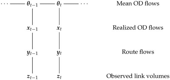
Figure 1.
Hierarchical relationship between variables in the DLM. Mean OD flows, realized OD flows and route flows are unobserved variables.
Let be the vector of realized OD flows at time t. We assume where is a covariance matrix, which can account for correlations between OD flows or simply be a diagonal matrix in case OD flows are independent. Given a realized vector , for each OD pair j, there is a vector of route flows , in which is the size of the route set of OD pair j, and let be the probability of route being selected at time t. We assume follows a multivariate normal distribution with a multinomial-like covariance structure, i.e.,
where and denote the expected value and the covariance, respectively. Thus, , in which is the vector of route choice probabilities of OD pair j and the covariance matrix is given by
where denotes a matrix whose diagonal elements correspond to the vector and all other elements are zero. Notice also that as , the covariance matrix will be singular and the corresponding multivariate normal distribution will be degenerate. In order to avoid this, we assume there is a positive probability of none of the routes in a route set being chosen, so that assuring that is non-singular. This assumption will be realistic if the route sets include many routes, so that flows on the excluded routes are negligible.
Let be the joint vector of route flows across all OD pairs. We also define as a block-diagonal matrix composed of route choice probability vectors and as a block-diagonal matrix composed of covariance matrices of route flows, i.e.,
Since we defined multivariate normal distributions for all subvectors , and assuming that route flow subvectors are conditionally independent given realized OD flow vector , we have that . (For convenience, we omit the explicit dependence on in the following developments).
Now, we are able to obtain the conditional by marginalizing . Since both the densities and are multivariate normal, and ignoring the dependence of on (we will take the dependence of on into account in the inference of in next section), from the properties of the multivariate normal [32], we have
In order to complete the formulation of our model, we must obtain the conditional density of observed traffic volumes given mean OD flows. First, we assume that , where is the covariance matrix of measurement errors when observing volumes on links. is the link-path incidence matrix for observed links, whose entries if link i make part of route k and , otherwise. It is a deterministic parameter which is a function of the topology of the network and of the route choice sets.
Since both and are multivariate normal, by marginalizing , we have
From Equation (6), we can finally specify and by defining
as an assignment matrix and the covariance matrix by
It is noteworthy in Equation (8) that the variability in OD flows, in route choices and in volume measurement are all represented in the covariance matrix. In the next section, we describe the estimation equations for mean OD flows.
2.1.2. Estimation of Mean OD Flows
Estimation of mean OD flows from observed link volumes can be made by Bayesian updating. We assume that the covariance matrices , and , the link-path incidence matrix , the route choice matrices and the probability of none of the routes in a route set being chosen are known parameters and are part of the prior knowledge.
At time t, let be the posterior distribution in the previous time step , where is the set of observed volume vectors in past time periods. We have a prior distribution before the observation of . Since, in our local constant model given by Equation (1), the system matrix , then
Notice that uncertainty on mean OD flows increases by addition of the evolution matrix to the covariance matrix . Next, we define as the one-step forecast distribution of the vector of observed link volumes, where
It is worth noting that, in computing by Equation (8), the covariance matrix of route flows is computed based on the predicted mean OD flows , i.e., in which from Equation (3)
Finally, the parameters of the posterior distribution are given by the Bayesian updating of the parameters, which in this case coincide with Kalman filter updating equations (see [31])
where is an adjustment matrix, which controls how the parameters from the posterior distribution are modified according to the new observation . In particular, the adjustment matrix is a function of the prior covariance matrix and of the inverse of the covariance matrix of the one-step forecast distribution of link volumes, so that the adjustment matrix gives more or less weight to observed link volumes according to their uncertainty relative to the uncertainty in OD flows.
At a time t, is an estimator of the mean OD flows and is a measure of uncertainty of the estimate. At , we define where are not actually observed link volumes but symbolically represents the modeler’s prior knowledge on OD flows. The estimation procedure can be summarized as follows:
- Starting from , set ;
- For to T, do:
- (a)
- (b)
- Compute the assignment matrix by means of Equation (7).
- (c)
- (d)
- (e)
In the next section, we model route choice probabilities based on a utility model in order to estimate jointly mean OD flows and the route choice matrix.
2.2. Bayesian Inference on Route Choice Parameters
In Section 2.2.1, we treat route choice probabilities as unobserved quantities and represent them through a utility model. In Section 2.2.2, we propose an MCMC algorithm to approximate the joint posterior distribution of route choice parameters and mean OD flows.
2.2.1. Utility Model and Route Choice Probabilities
In congested networks, route choice probabilities greatly depend on past route costs. Users take into account their previous experiences in order to evaluate the utility associated with each route. Utilities will vary over time depending on user’s memory, their sensitivity to route costs, fluctuations in mean OD flows, among other possibly influencing factors. As route choice probabilities are functions of utilities, these will also dynamically change.
We assume that the utility of a route k in an OD pair j at a time t as perceived by users is a linear function of its past route that costs
are parameters, are observed past route costs and r is the length of users’ memory. The minus sign in Equation (17) is used since costs are disutilities, in order that routes with lower costs are preferable. We may interpret the parameters as users’ sensitivities to past route costs. It is reasonable to assume that they have non-negative values; otherwise, higher costs will contribute to higher utilities. We also expect users to be more sensitive to recent route costs than to older costs, which implies that .
We adopt a multinomial logit model for route choice probabilities [33] in order that the probability of a route in OD pair j at time t being chosen by a user is given by
where is the probability of a user not following a route in a route choice set and e denotes Euler’s number.
2.2.2. An MCMC Algorithm
In this section, we develop an MCMC algorithm in order to sample from the joint posterior distribution of mean OD flows and the parameters of the route choice utility model given in (17).
From Bayes theorem, we have:
where is a shorthand referring to the vectors and a shorthand for . is the joint posterior, is the likelihood function of the observed link volumes and is the prior distribution. We include in prior knowledge set all other parameters, such as for , and route costs for .
We notice that Gibbs sampling [34] allows us to sample from the joint distribution by alternately sampling from conditional distributions and . We must then devise how to sample from each distribution.
Sampling from can be implemented through the forward filtering backward sampling (FFBS) method [31,35,36]:
- (backward sampling) Starting from , for , sample each backwards from the conditionals , in which:and . We notice that step 1 (forward filtering) of the FFBS algorithm is possible since, given , observed link volumes and prior knowledge , we have the route choice matrix and all other parameters determined for , so that we can apply recurrence Equations (14) and (15). Then, step 2 generates a sample of mean OD flows .
Regarding the conditional , sampling can be performed through a Metropolis–Hastings (MH) step [37]. First, we notice that:
as does not depend on , and is the prior distribution of . From (6), the likelihood term is given by:
in which matrices and are dependent on since they are functions of the route choice matrices , which are dependent on through Equations (17) and (18).
The MH step is then performed as follows: given a candidate vector , where is the current vector at iteration i and is a proposal distribution, sample and accept as next sample if:
otherwise, make .
Finally, the proposed MCMC algorithm is summarized below:
- Initialize vectors and .
- From iteration onwards, repeat until convergence:
In the next section, we illustrate the application of the proposed MCMC algorithm through some numerical studies.
3. Results and Discussion
In the following subsections, we describe the generation of simulated data and present the results from the application of our approach to a test network from the literature.
3.1. Generation of Simulated Data
In order to illustrate the application of our proposed DLM and MCMC algorithm, we generated data for a transportation network from [28], given in Figure 2, which has eight nodes and 10 links. Nodes 1 and 2 are the origins and nodes 7 and 8 are the destinations, so that we have four OD pairs: (1,7), (1,8), (2,7) and (2,8).
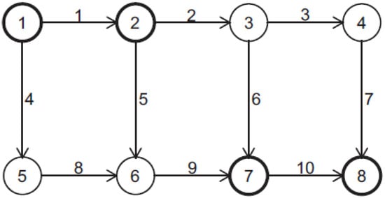
Figure 2.
Network used in the numerical studies (adapted from [28]).
In order to adapt the network to our experiment, we did not use the original data on demand and link parameters. We assumed that travel times on links are given by BPR functions according to Equation (25):
where is the travel time on a link with traffic volume z, denotes the travel time in “free flow” and is the capacity of the link. and are parameters of the function, for which we adopt the typical values from the literature 0.15 and 4, respectively [38]. Note that the capacity of the link is not treated as a hard constraint, i.e., simulated volumes z are allowed to be greater than . In the test network, we set and on all links. The procedure used to generate the simulated data was the following:
- At , set values for , , , , , , for to T and past route costs , where r is the size of users’ memory and denotes route costs computed assuming free flow in the network.
- For to T do:
OD flows vary within the interval and follow the locally constant model given in Equation (1), starting at time from the OD flow vector . The OD pairs are ordered lexicographically in vector , so that mean OD flows in OD pair (1,7) corresponds to , (1,8) corresponds to and so on. The evolution covariance matrix is constant and given by , where is the appropriate identity matrix. We assume that variability around mean OD flows is negligible, so as to and for all t, and we also assume that . These assumptions imply that variability in observed link volumes will be mostly due to variability in route choices. We simulate OD flows for time periods.
In addition, we set a users’ memory length of for the utility model, so that utility of a route k of OD pari j at time t is given by (Equation (17)) and is the vector of route choice parameters. We enumerated exhaustively all 12 routes between origins and destinations, resulting in a link-path incidence matrix with 10 rows and 12 columns. Since we enumerated all routes, we assumed a small probability of a trip not following one of the routes. Table 1 shows the mean congestion level (CL) for a link i, given by the ratio between mean simulated traffic volumes and the link capacities:

Table 1.
Mean congestion level (CL) on links from simulated OD flows.
As can be seen in Table 1, links 2, 5, 6 and 9, which are in the central area of the network, have high congestion levels.
The simulations, the proposed DLM and MCMC algorithm were implemented in the Python programming language version 2.7 by using Numerical Python module version 1.10.
3.2. Application of the MCMC Algorithm
When applying the MCMC algorithm, we assume that we observe link volumes on all links and route costs . In practice, these data on traffic volumes are routinely collected through modern ITS systems and route costs can be estimated from data on travel times on links or can be collected from a sample of cars following selected routes. Except for the mean OD flows and the parameters , we assume all other parameters are known. We use an uninformative multivariate normal prior for the initial mean OD flows vector , with , where is the unit vector with the appropriate dimension and , and an uninformative improper prior for .
The MCMC algorithm was ran through 10,000 iterations with a multivariate normal proposal distribution for candidate vectors with covariance matrix equals to , which resulted in an acceptance percentage of about 22%, and we discarded the initial 2000 samples as burn-in. We used as starting values for and the starting values for are sampled from a multivariate normal with mean and covariance matrix . It took about 10 min to run the MCMC algorithm in an Intel Core i7 machine with 3.1 GHz and 8GB RAM.
The resulting Markov chain of sampled values is given in Figure 3. Figure 4 shows kernel density estimation of the marginal posteriors of and obtained from the sampled values. It can be seen that the sampled marginal posteriors have high densities around the true simulated values for and . The sample mean values for and were 0.5250 and 0.3651, respectively, and highest posterior density regions with 95% probability were (0.3546, 0.7067) and (0.1979, 0.5437), respectively. Figure 5 shows the simulated and estimated mean OD flows, with mean squared error (MSE) between simulated and estimated mean OD flows of 15.83. From these results, we can conclude that the proposed MCMC algorithm was able to estimate with good accuracy both mean OD flows and route choice parameters.
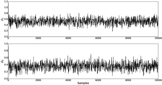
Figure 3.
Markov chain for and .
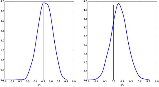
Figure 4.
Kernel density estimation for the marginal posteriors of and . Vertical axes show probability density. Vertical bars show true simulated values.
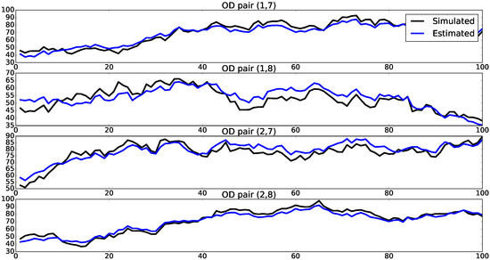
Figure 5.
Simulated and estimated mean OD flows. Horizontal axes show time periods, while vertical axes show magnitude of OD flows.
3.3. Unknown Evolution Matrix
Although in theory the evolution matrix in DLMs may be jointly estimated along with other parameters, it is often treated as a known parameter provided by the analyst. A convenient way of specifying the evolution matrix is through discount factors [31]. According to Equation (9), the prior covariance matrix of the OD flows at time t is given by , i.e., it is the posterior covariance matrix at the previous time period amplified by the evolution covariance matrix, which corresponds to the increase in uncertainty due to time. Then, we can write the prior covariance matrix as , where , so as to . The term is a discount factor. Notice that, when , we do not have an increase in uncertainty from time to t, thus corresponding to a static model. Lower values correspond to higher increase in uncertainty from time to time t.
We ran our proposed MCMC algorithm with varying discount factors , starting from covariance matrix , in order to assess its impact on the quality of the estimation of the route choice parameters and mean OD flows. In Table 2, we show the corresponding sample means and , 95% highest posterior density (HPD) regions for and , and mean squared error (MSE) between simulated and estimated mean OD flows.
Table 2.
Estimation results given different discount factors (HPD—95% highest posterior density region).
Figure 6 illustrates the effect of using on the estimation of mean OD flows. As can be seen from the results, there was little difference in estimation quality between the cases with known and unknown evolution matrix regarding the parameters . The difference is more pronounced with relation to estimation quality of mean OD flows, which exhibited higher MSE with the evolution matrix specified by means of a discount factor.
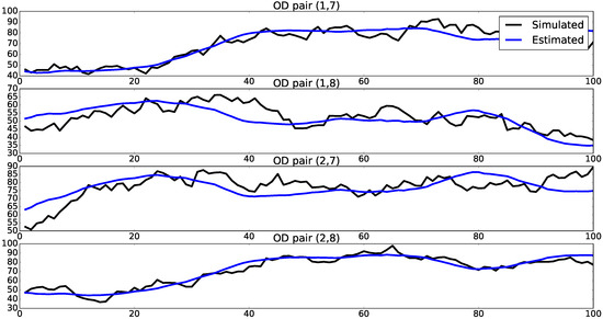
Figure 6.
Simulated and estimated mean OD flows for . Horizontal axes show time periods, while vertical axes show magnitude of OD flows.
3.4. Observation of Traffic Volumes on Partial Links
In some real transportation networks, there are data on traffic volumes only on a few links. We consider the application of our MCMC algorithm in these settings. In this set of experiments, all parameters are equal to the simulated ones, except for the mean OD flows and the parameters of the utility model, which are estimated by the MCMC algorithm. We vary only the number of links and in which of them we have traffic volume data.
We test three cases: observations on one link, on two links, and on three links in the network in Figure 2. Links were selected so that we have a representative subset of the network. In Table 3, we show the corresponding sample means and , 95% highest posterior density regions for and , and MSE between simulated and estimated mean OD flows.
Table 3.
Estimation results with observation on partial links (HPD—95% highest posterior density region).
In Table 3, we see that MSE of mean OD flows decreases as we observe more links. This result is in agreement with similar results of experiments with static models in the literature. The best results were obtained with data on links 1, 7 and 9, for which . It is noteworthy that this result is not very far from the case studied in Section 3.2, where we have traffic volume data on all links and . Figure 7 shows simulated and estimated mean OD flows for this case with data on links 1, 7 and 9.
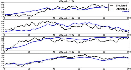
Figure 7.
Simulated and estimated mean OD flows with observed traffic volumes on links 1, 7 and 9. Horizontal axes show time periods, while vertical axes show magnitude of OD flows.
Estimation quality of route choice parameters also increases with the observation of more links, as the HPD regions get tighter around the simulated values . Nevertheless, this effect is not so pronounced for OD flows. The best result among the tested cases was obtained when observing links 2, 5 and 9, which are links located in the central and more congested region of the network. It is also worth noting that we could estimate route choice parameters to a good accuracy by observing only link 9.
In addition, we notice that the estimation results for the case when we have traffic volumes data only on link 1 are the worst. This may be possibly due to the fact that there is no route in OD pairs (2,7) and (2,8) which includes link 1. Thus, traffic volumes on link 1 give no information on OD flows for these OD pairs. In Figure 8, we see that estimated mean OD flows remain at 100 in this case, which is our prior mean at .
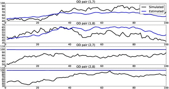
Figure 8.
Simulated and estimated mean OD flows with observed traffic volumes on link 1. Horizontal axes show time periods, while vertical axes show magnitude of OD flows.
Finally, we should emphasize that we obtained good estimates when observing only a subset of links even though we used uninformative priors for both mean OD flows and route choice parameters. Static models often resort to prior knowledge, in the form of prior OD matrices, in order to “regularize” estimates when data are available only on a few links.
4. Conclusions
In this paper, we proposed a dynamic linear model for day-to-day OD flows in transportation networks. In our model, we took into account variability in OD flows, route choices and traffic volume measurements. We also modeled route choices through a utility model based on past route costs. We proposed a Markov chain Monte Carlo algorithm in order to sample from the joint posterior distribution of mean OD flows and route choice parameters by using data on traffic volumes on links and past route costs. Our model can be applied to congested networks and when data are available on only a subset of links.
We illustrated the application of the DLM and MCMC algorithm on a test network from the literature using simulated data. In our experiments, we were able to estimate with good accuracy both mean OD flows and route choice parameters using uninformative prior distributions and data on a subset of links in the test network. These are very promising results and indicate that dynamic linear modeling of day-to-day OD flows may provide a valuable tool in analyzing and estimating OD demand in transportation networks. Although we carried out computational experiments on a small network, due to the convenience of testing the model and presenting the results, we made no limiting assumptions on the size of the network when developing the model and algorithm, so that it may be applied to networks of any size.
As further extensions to our work we suggest the consideration of trend and seasonality in OD flows. This can be implemented through the definition of additional parameters such as trend and seasonal factors, whose relationship with mean OD flows can be easily established by means of the system matrix . Another promising research direction is the use of our proposed DLM to forecast future traffic volumes, after setting up the model with estimated route choice parameters.
Author Contributions
Conceptualization and Methodology by all the authors; Writing—Original Draft Preparation, A.R.P.-N.; Writing—Review and Editing by all the authors.
Funding
This research was funded by Conselho Nacional de Desenvolvimento Científico e Tecnológico, Grant No. 422464/2016-3.
Conflicts of Interest
The authors declare no conflict of interest. The founding sponsors had no role in the design of the study; in the collection, analyses, or interpretation of data; in the writing of the manuscript, and in the decision to publish the results.
Nomenclature
In the text and in the equations, lowercase italic letters represent scalars, while vectors are represented by bold lowercase letters and matrices by uppercase bold letters. Greek letters are in general reserved to parameters, but there are exceptions such as some covariance matrices which are represented by the Greek capital letter . Sets are typed in calligraphic letters, while blackboard letters (such as ) denote probability density functions. We provide below a list of symbols used in the paper:
| Vector of mean OD flows at time t; | |
| Vector of realized origin–destination (OD) flows at time t; | |
| Vector of route flows at time t; | |
| Vector of traffic volumes on links at time t; | |
| Vector of route choice probabilities at time t; | |
| Vector of route costs at time t; | |
| Set of routes for OD pair i; | |
| Vector of parameters in the utility equation of a route given past route costs; | |
| Probability of not using a route in a given route choice set; | |
| Performance (cost) function of a link; | |
| Vector of random errors in the observational model at time t; | |
| Vector of evolution errors in the as the dynamic model at time t; | |
| State evolution matrix (system matrix); | |
| Assignment matrix at time t; | |
| Evolution covariance matrix of mean OD flows at time t; | |
| Covariance matrix of traffic volumes on links at time t; | |
| A covariance matrix at time t; | |
| Route choice matrix at time t; | |
| A link-path incidence matrix; | |
| v | Location vector of the prior distribution of mean OD flows at time t; |
| Covariance matrix of the prior distribution of mean OD flows at time t; | |
| Location vector of the posterior distribution of mean OD flows at time t; | |
| Covariance matrix of the posterior distribution of mean OD flows at time t; | |
| The identity matrix; | |
| A matrix whose main diagonal is the vector and entries off the main diagonal are all zero; | |
| A block-diagonal matrix composed of submatrices ; | |
| Multivariate normal distribution with mean vector and covariance matrix ; | |
| Multinomial distribution with parameters x and . |
References
- De Dios Ortúzar, J.; Willumsen, L. Modelling Transport, 4th ed.; Wiley: Chichester, UK, 2011. [Google Scholar]
- Cascetta, E. Transportation Systems Analysis: Models and Applications, 2nd ed.; Springer: New York, NY, USA, 2009. [Google Scholar]
- Robillard, P. Estimating the OD matrix from observed link volumes. Transp. Res. 1975, 9, 123–128. [Google Scholar] [CrossRef]
- Nguyen, S. Estimating an OD Matrix from Network Data: A Network Equilibrium Approach; Technical Report; Centre de Recherche sur les Transports, Université de Montreal: Montreal, QC, Canada, 1977. [Google Scholar]
- Beckmann, M.; McGuire, C.; Winsten, C.B. Studies in Economics of Transportation; Yale University Press: Ann Arbor, MI, USA, 1956. [Google Scholar]
- Van Zuylen, H.J.; Willumsen, L.G. The most likely trip matrix estimated from traffic counts. Transp. Res. Part B 1980, 14, 281–293. [Google Scholar] [CrossRef]
- Cascetta, E. Estimation of Trip Matrices from Traffic Counts and Survey Data: A Generalized Least Squares Estimator. Transp. Res. Part B 1984, 16, 289–299. [Google Scholar] [CrossRef]
- Cascetta, E.; Nguyen, S. A unified framework for estimating or updating origin/destination matrices from traffic counts. Transp. Res. Part B 1988, 22B, 437–455. [Google Scholar] [CrossRef]
- Brenninger-Göthe, M.; Jörnsten, K.O. Estimation of origin–destination matrices from traffic counts using multiobjective programming formulations. Transp. Res. Part B 1989, 23B, 257–269. [Google Scholar] [CrossRef]
- Fisk, C. On combining maximum entropy trip matrix estimation with user optimal assignment. Transp. Res. Part B 1988, 22B, 69–79. [Google Scholar] [CrossRef]
- Fisk, C. Trip matrix estimation from link counts: the congested network case. Transp. Res. Part B 1989, 23B, 331–336. [Google Scholar] [CrossRef]
- Wardrop, J.G. Some theoretical aspects of traffic research. In Proceedings of the Institution of Civil Engineers Part II; Institution of Civil Engineers: London, UK, 1952; Volume 1, pp. 325–378. [Google Scholar]
- Smith, M. The existence, uniqueness and stability of traffic equilibria. Transp. Res. Part B 1979, 13B, 295–304. [Google Scholar] [CrossRef]
- Yang, H.; Sasaki, T.; Iida, Y.; Asakura, Y. Estimation of origin–destination matrices from link counts on congested networks. Transp. Res. Part B 1992, 26B, 417–434. [Google Scholar] [CrossRef]
- Yang, H. Heuristic algorithms for the bilevel origin–destination matrix estimation problem. Transp. Res. Part B 1995, 29B, 231–242. [Google Scholar] [CrossRef]
- Cascetta, E.; Postorino, N. Fixed point approaches to the estimation of O/D matrices using traffic counts on congested networks. Transp. Sci. 2001, 35, 134–147. [Google Scholar] [CrossRef]
- Sheffi, Y. Urban Transportation Networks: Equilibrium Analysis with Mathematical Programming Methods; Prentice-Hall: Englewood Cliffs, NJ, USA, 1985. [Google Scholar]
- Vardi, Y. Network tomography: Estimating source-destination traffic intensities from link data. J. Am. Stat. Assoc. 1996, 91, 365–377. [Google Scholar] [CrossRef]
- Tebaldi, C.; West, M. Bayesian inference on network traffic using link count data. J. Am. Stat. Assoc. 1998, 93, 557–573. [Google Scholar] [CrossRef]
- Hazelton, M.L. Estimation of origin–destination matrices from link flows on uncongested networks. Transp. Res. Part B 2000, 34, 549–566. [Google Scholar] [CrossRef]
- Hazelton, M.L. Some comments on origin–destination matrix estimation. Transp. Res. Part A 2003, 37, 811–822. [Google Scholar] [CrossRef]
- Hazelton, M.L. Inference for origin–destination matrices: Estimation, prediction and reconstruction. Transp. Res. Part B 2001, 35, 667–676. [Google Scholar] [CrossRef]
- Cremer, M.; Keller, H. A new class of dynamic methods for the identification of origin–destination flows. Transp. Res. Part B 1987, 21, 117–132. [Google Scholar] [CrossRef]
- Cascetta, E.; Inaudi, D.; Marquis, G. Dynamic estimators of origin–destination matrices using traffic counts. Transp. Sci. 1993, 27, 363–373. [Google Scholar] [CrossRef]
- Ashok, K.; Ben-Akiva, M.E. Estimation and prediction of time-dependent origin–destination flows with a stochastic mapping to path flows and link flows. Transp. Sci. 2002, 36, 184–198. [Google Scholar] [CrossRef]
- Hazelton, M.L. Statistical inference for time varying origin–destination matrices. Transp. Res. Part B 2008, 42, 542–552. [Google Scholar] [CrossRef]
- Parry, K.; Hazelton, M. Bayesian inference for day-to-day dynamic traffic models. Transp. Res. Part B 2013, 50, 104–115. [Google Scholar] [CrossRef]
- Hazelton, M.L.; Parry, K. Statistical methods for comparison of day-to-day traffic models. Special issue: Day-to-Day Dynamics in Transportation Networks. Transp. Res. Part B: Methodol. 2016, 92, 22–34. [Google Scholar] [CrossRef]
- Watling, D.P.; Cantarella, G.E. Modelling sources of variation in transportation systems: Theoretical foundations of day-to-day dynamic models. Transp. B Transp. Dyn. 2013, 1, 3–32. [Google Scholar] [CrossRef]
- Cantarella, G.E.; Watling, D.P. Modelling road traffic assignment as a day-to-day dynamic, deterministic process: A unified approach to discrete- and continuous-time models. EURO J. Transp. Logist. 2015, 5, 69–98. [Google Scholar] [CrossRef]
- West, M.; Harrison, J. Bayesian Forecasting and Dynamic Models, 2nd ed.; Springer: New York, NY, USA, 1997. [Google Scholar]
- Särkkä, S. Bayesian Filtering and Smoothing; Cambridge University Press: New York, NY, USA, 2013. [Google Scholar]
- Ben-Akiva, M.; Lerman, S.R. Discrete Choice Analysis: Theory and Application to Travel Demand; MIT Press: Cambridge, MA, USA, 1985. [Google Scholar]
- Geman, S.; Geman, D. Stochastic Relaxation, Gibbs Distributions, and the Bayesian Restoration of Images. IEEE Trans. Pattern Anal. Mach. Intell. 1984, PAMI-6, 721–741. [Google Scholar] [CrossRef]
- Carter, C.K.; Kohn, R. On Gibbs Sampling for State Space Models. Biometrika 1994, 81, 541–553. [Google Scholar] [CrossRef]
- Frühwirth-Schnatter, S. Data augmentation and dynamic linear models. J. Time Ser. Anal. 1994, 15, 183–202. [Google Scholar] [CrossRef]
- Hastings, W.K. Monte Carlo sampling methods using Markov chains and their applications. Biometrika 1970, 57, 97–109. [Google Scholar] [CrossRef]
- Bureau of Public Roads. Traffic Assignment Manual for Application with a Large, High Speed Computer; U.S. Departmnet of Commerce, Bureau of Public Roads, Office of Planning, Urban Planning Division: Washington, DC, USA, 1964. [Google Scholar]
© 2018 by the authors. Licensee MDPI, Basel, Switzerland. This article is an open access article distributed under the terms and conditions of the Creative Commons Attribution (CC BY) license (http://creativecommons.org/licenses/by/4.0/).