Article

Assessing Active Living Potential: Case Study of Jacksonville, Florida

Department of Urban and Regional Planning, College of Design, Construction, and Planning, University of Florida, Gainesville, FL 32611, USA
Urban Sci. 2018, 2(2), 44; https://doi.org/10.3390/urbansci2020044
Submission received: 19 April 2018 / Revised: 24 May 2018 / Accepted: 28 May 2018 / Published: 29 May 2018

Abstract

:
Many municipalities in the US are deploying urban planning approaches to resolve problems caused by urban sprawl, particularly the lack of support for physical activity. Although a variety of perspectives on the relationship between physical activity and built environment exist, many studies have suggested objective and reliable measures of urban form that encourage more opportunities for physical activity. Thus, based on the research context, this study builds a Geographic Information System (GIS) model using geospatial dimensions, yields a visualized map ranked by composite scores, and reveals the spatial distribution of quantified cells. Through the Jacksonville case study, it is shown that the GIS-based visualization method provides an expanded set of tools that can help urban planners and public health professionals understand the relationships between urban form and potential for active living. Consequently, these map-based visualized results provide valuable information to health and public policy professionals to coordinate and resolve mutual challenges.

1. Introduction

The predominance of obesity and diabetes have increased drastically across the US over the last two decades [1,2]. Among various causes of obesity and diabetes, several public health researchers found that physical inactivity is one of the common factors [2,3]. In consideration of this issue, urban planning studies have tried to identify the relationship between physical activity and built environment. Numerous studies have found that certain urban form features—land use mixed level, accessibility to open space, well-connected sidewalks—have positive associations with physical activity levels [4,5,6,7,8]. Particularly, several scholars found that urban sprawl, which is an urban form pattern that reflects low-density housing development and automobile-dependency on the fringe of an existing urban area, is positively associated with the risk of being obese and being physically inactive [9,10,11,12]. Although positive association between built environment and physical activity might not imply causation, studies have suggested that active built environment, which refers to urban form that could encourage physical activity, is essential to creating and maintaining a healthier society [13,14,15].
Along with these contexts, a main research question is posed: Which locations have more active living potential than other areas? To answer this question, a comprehensive active built environment index will be developed, which includes multiple operationalized variables that may affect the physical activity of residents. Also, additional questions are established: first, which areas have more potential for active living; second, which residential types (e.g., single-family housing, multifamily housing) have a higher active living potential; third, which residential types are highly clustered with higher opportunities for active living. While the initial question simply finds areas having active living potential, these additional questions could demonstrate the capability of the method as a potential toolset that can be used by policymakers, urban planners, and public health professionals to support the physical activity of residents.
Thus, the objectives are as follows: first, operationalize Geographic Information System (GIS) variables, which represent geospatial dimensions of active built environment; second, develop a GIS model to assess urban forms, which means that the output of the model answers which locations have more active living potential than others; third, apply the modeling results to parcel-level data for responding to the research questions.
Although the relationships between built environment and human behavior, especially physical activity, vary by context and encompass multiple aspects, several researchers tried to identify urban form variables that affect physical activity from about 50 archival research papers [16]. They found several common variables to affect potential physical activity, including land use mixed level, accessibility to destinations, and street patterns.
Since land use directly defines urban forms, numerous studies have tried to identify relationships between land use and physical activity. Specifically, several studies showed how mixed-use development has a robust and positive relationship with physical activity; people are more likely to walk if they live in mixed-used neighborhoods with parks, schools and commercial destinations nearby [4,5,17].
Other studies suggested that the distance to destinations is a crucial part of active living. First, full-size grocery stores in neighborhoods positively correlate with healthier diet and weight among residents [18,19]. Second, proximity to schools significantly enhances children’s levels of activity. A study supported this argument by reporting that youth who live within half a mile of a school had a greater likelihood of walking or biking to school [20]. Third, researchers have argued for the significance of proximity to recreational spaces such as parks, public spaces, and recreational facilities with regard to active living. The optimal distance varies, but people who live closer to recreational spaces are more likely to visit the spaces and exercise more often [6,21,22,23,24,25].
Active transportation modes such as walking and bicycling have also played a significant role in providing more physical activity opportunities [26]. Public transit is an important variable that encourages walking for both adults and children [27,28,29]. Moreover, a lot of studies have stressed the significance of streets as a walk space [30,31,32,33,34,35,36,37,38]. Regarding the bicycling, a well-connected network of bicycle infrastructure is positively associated with physical activity using bicycles [39]. Also, another study showed that obesity rates of frequent bicycle users are lower in countries that have accessible bicycle infrastructure [40].
Along with the significance of identifying the relationship between geospatial variables of active living and physical activity, recent studies have tried to assess active built environments, especially the walkability of a built environment. Since walkability is a crucial part of physical activity, there are various attempts to develop new indicators, building on issues with the conventional walkability measures. The typical method to measure walkability is Walk Score, which, using a scale of 0 to 100, calculates a score by considering walking distance to amenities, population density, block length, and intersection density. This score has been shown to be a valid measurement of walkability in multiple geographic locations [41,42]. Another method to measure destination accessibility is the Neighbourhood Destination Accessibility Index (NDAI), which is a measure of pedestrian access to neighborhood destinations [43]. The NDAI was derived by computing a score for each destination (a binary score of 0 or 1 was assigned according to whether the destination was present or absent within the 800 m buffer) and then combined into a single domain score. While previous studies mainly considered destinations, the Pedestrian Environment Index (PEI)—which consists of four parts including land-use diversity based on entropy index, population density, commercial density, and intersection density—was developed to measure pedestrian friendliness for urban neighborhoods [44]. The PEI combines four components by multiplication since factors affecting the pedestrian environment are subject to cause-and-effect (i.e., a change in one factor could result in changes in the other factors). The PEI falls between 0 and 1, and the maximum means a built environment could better support pedestrian activities. Another study concluded that considering both residential density and the walkable destinations creates good measures of urban walkability and can be recommended for use by policy-makers, planners and public health officials [45]. However, an additional study suggested the Space Syntax Walkability (SSW) method, which employs gross population density and a space syntax measure of street integration, could provide a toolset for further understanding of how urban design makes an impact on walking behaviors [46]. The authors argued that, compared to conventional walkability measures, the SSW method appears to be an effective alternative to full walkability in terms of data availability and processing.
Since both types of studies, which include identifying variables of active built environment and objectively measuring built environment for active living, have recognized the lack of objective measurement of active built environment, they suggested that objective and reliable measures of active built environment would be more efficient for both urban planning and public health studies [16,19,43,47,48]. Using the capability of GIS is considered an especially feasible way to generate objective measures for studies of individuals and neighborhoods.

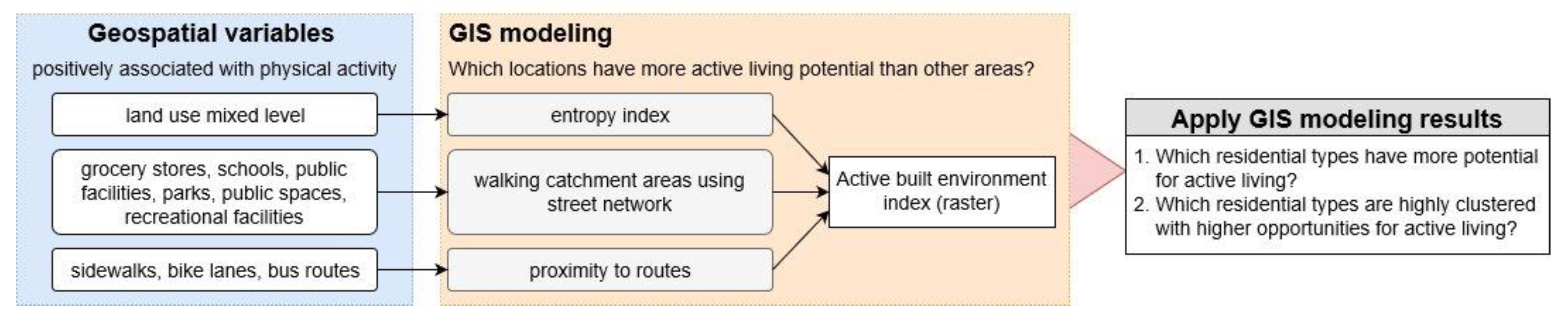
2. Materials and Methods

The study was undertaken in Jacksonville, Florida, which was selected because Jacksonville is the largest city and has one of the highest diabetes ratios in Florida [49]. Aforementioned in the previous section, diabetes is positively associated with physical inactivity. Therefore, Jacksonville might be a city that has a lower physical activity level among its residents than other cities in Florida. Another reason to choose Jacksonville is that detailed and required GIS data are available for the city.
Despite complexities inherent in urban forms and physical activity, a considerable number of studies have shown positive relationships between physical activities and certain geospatial dimensions such as mixed land use, proximity to destinations, and active transportation modes. Especially, the destinations include grocery stores, schools and recreational space (e.g., parks, public spaces, public facilities, and recreational facilities). The active transportation modes comprise of walking using sidewalks, bicycling using bike lanes, and walking to public transit.
The following show used data descriptions and their sources. For computing land use mixed level, land use and census data are used. I obtain land use data from the Florida Department of Transportation (FDOT), which maintains generalized land use derived from parcels. For census data, 2010 census block boundaries from the US Census Bureau are used. For the identified destinations, parcel-level data is employed, which include the specific use of each parcel from the Florida Department of Revenue (FDOR) land use classification. I obtain the parcel data from the Florida Geographic Digital Library (FGDL). The detailed descriptions of each destination are as follows:
  • Grocery stores: supermarkets, neighborhood or community shopping centers
  • Schools: public schools or colleges
  • Public facilities: facilities operated by municipalities other than public schools, colleges, military, or correctional facilities
  • Recreational facilities: theaters, auditoriums, or sport facilities
  • Parks: public parks
  • Public spaces: outdoor recreational spaces other than parks
It should be noted that it is possible to use the aforementioned destinations combined as one variable or several variables. However, since each destination could represent unique walk or physical activity opportunities, detailed levels of parcel data are employed instead of using a single variable. Also used is public transit information from the Florida Transit Information System (FTIS) and bike lane features from the Road Characteristics Inventory (RCI) of FDOT. Regarding sidewalks, Florida’s unified street data is employed, which contains detailed street networks and a functional classification of roads.
Since factors affecting physical activity are not a single and unified dimension, the proposed methodology requires the capability to handle complex datasets. Thus, to analyze multivariable geospatial data, a suitability model is employed since it works well with multipart hierarchical variables and larger datasets using rasterized layers [50]. Since raster layers consist of cells arranged in rows and columns and is a commonly used dataset in GIS, the rasterized layers could be used to represent geographic information and could also be used in raster-based modeling and analysis. Additionally, suitability modeling can provide several benefits. First, since studies sometimes failed to investigate regional contexts, suitability modeling is helpful in visualizing spatial patterns of active built environment within regional contexts. Second, the suitability model not only effectively handles large and complex data, but it also has the flexibility to add or remove relevant dimensions that consist of an active built environment.
Before starting the modeling, determining the proper cell size for analysis is critical because the cell size affects resolution of results, model performance, and disk storage requirements. Therefore, a 5-m cell size is used to capture the details of urban forms as well as to maximize workstation performance in ArcGIS.
Figure 1 illustrates the conceptual process of this study to develop a method to measure active living potential using variables identified from previous research. First, I identify the geospatial variables that positively associated with physical activity. Second, the model starts to convert each identified variable into a suitability layer by type of measurement. Based on the characteristics of each variable, three types of measurements—entropy index, walking catchment areas using street network, and proximity to routes—are used in the model. After generating individual layers, the model merges the layers into a single raster layer to show active built environment index, which represents active living potential of the study area. Last, using the parcel data as a boundary, it computes average scores of active built environment index. As a result, each parcel has a score to show active living potential.
Based on the nature of the variables and measurements, the first step establishes the three types of measurements. The first measurement is entropy index. Entropy index is used to represent land use mixed level since this measurement is one of the most common methods in geography and urban planning [51]. Using the census block boundary and land use data, the entropy index is calculated using a portion of the land use and the unique land use count. As a result, each census block shows values between 0 and 1. The entropy index is set at 1 when land use is maximally diverse and set at 0 when land use is maximally homogeneous. At the end of this measure, the vector layer is converted into raster layer.
The second measurement is walking catchment areas from destinations. This measurement is used to determine pedestrian proximity to identified destinations such as grocery stores, schools, parks, public spaces, public facilities, and recreational facilities. Thus, pedestrian proximity determines the level of measurement for the variables above (i.e., grocery stores, schools, parks, public spaces, public facilities, and recreational facilities). For example, the measurement for grocery stores is generating network walking catchment areas by 5-min walking distance from grocery stores since walking is the most efficient and common way to achieve a recommended level of physical activity in everyday life. However, it should be noted that walking possibility is not a simple linear relationship with waking distance. That is, defining specific ranges such as only within 5 min walking distance as the most suitable value might be difficult because some residents who live more than 5 min walking distance from a grocery store might still walk there. Because of missing “walking opportunity”, a fuzzy membership is employed during the rasterizing process. The fuzzy membership tool allows for specifying the likelihood that a given value is a member of a set rather than just deciding if the value is either inside or outside the set [52,53]. In other words, as the distance from a grocery store decreases, a person is more likely to walk to it, so the locations are more likely to be members of the suitable set. Thus, a new layer is created with corresponding fuzzy membership values rating from 1 to 0, accordingly. In here, 1 could represent the highest opportunity to walk. Another benefit of using fuzzy membership is that the output value is on the same scale as the entropy index, which ranges from 0 to 1. This common scale simplifies the overlay process and helps avoid the need to reclassify data. Since this study looks at active living potential, presenting walking possibility instead of simple distance from each destination is appropriate. Thus, regarding the destination variables (i.e., grocery stores, schools, parks, public spaces, public facilities, and recreational facilities), fuzzy membership is utilized to create suitability layers and output layers showing values from 0 to 1.
The last measurement is used to determine proximity based on whatever transportation options are available such as public transit, sidewalks, and bikeways. Both public transit routes and pedestrian pathways are used for assessing potential walkability, and bikeways are used for finding potential physical activities via bike usage. For example, to create a public transit suitability, the model creates walking catchment areas by 5-min walking distance from bus routes. However, for the bike lane, this study uses ½-mile and 1-mile buffers from bikeways since biking is another way to achieve physical activity. At the end of each process, a suitability layer is created using the fuzzy membership, which has value between 0 and 1.
After creating individual suitability layers, the last step in this model is combining the outputs from the previous individual processes and generating an active built environment index. The cells with combined high scores represent locations with higher suitability for physical activity. Because 10 variables are used and the maximum score of each variable is 1, a perfect score representing the maximum potential for physical activity would be 10. During the composite scoring process, though this study does not use any weights by variables, weighting layers differently based on importance is generally possible.
Finally, using the active built environment index, there is a possibility for another type of spatial analysis. Since the cell size of the active built environment index map is 5 m, these cells can be applied to each parcel. Using the zonal statistic function, the average value of the scored cells that belong to the parcel is assigned. The average value of each parcel is used for responding to the research questions: which residential types have more active living potential and how is active living potential clustered by residential types.

3. Results

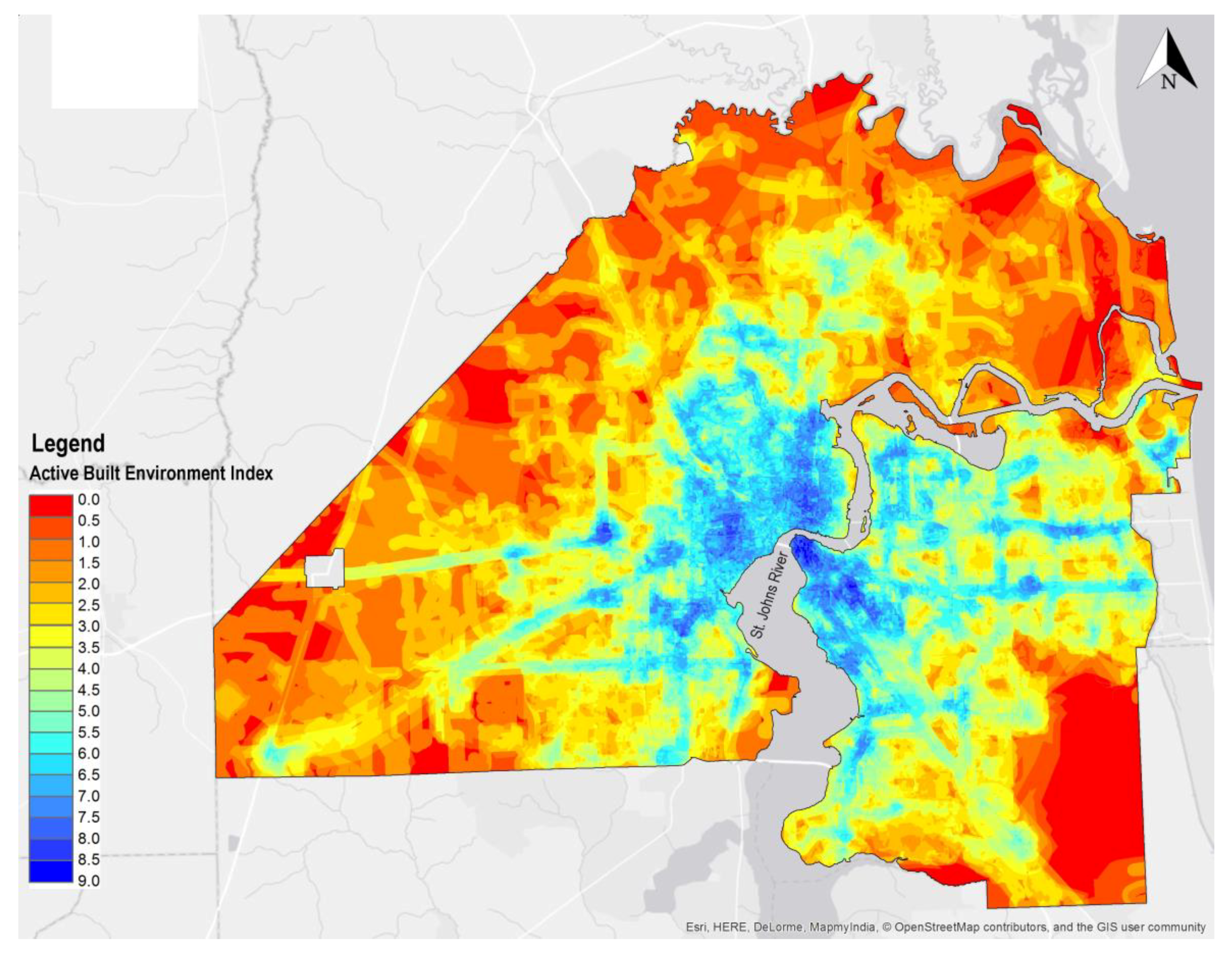
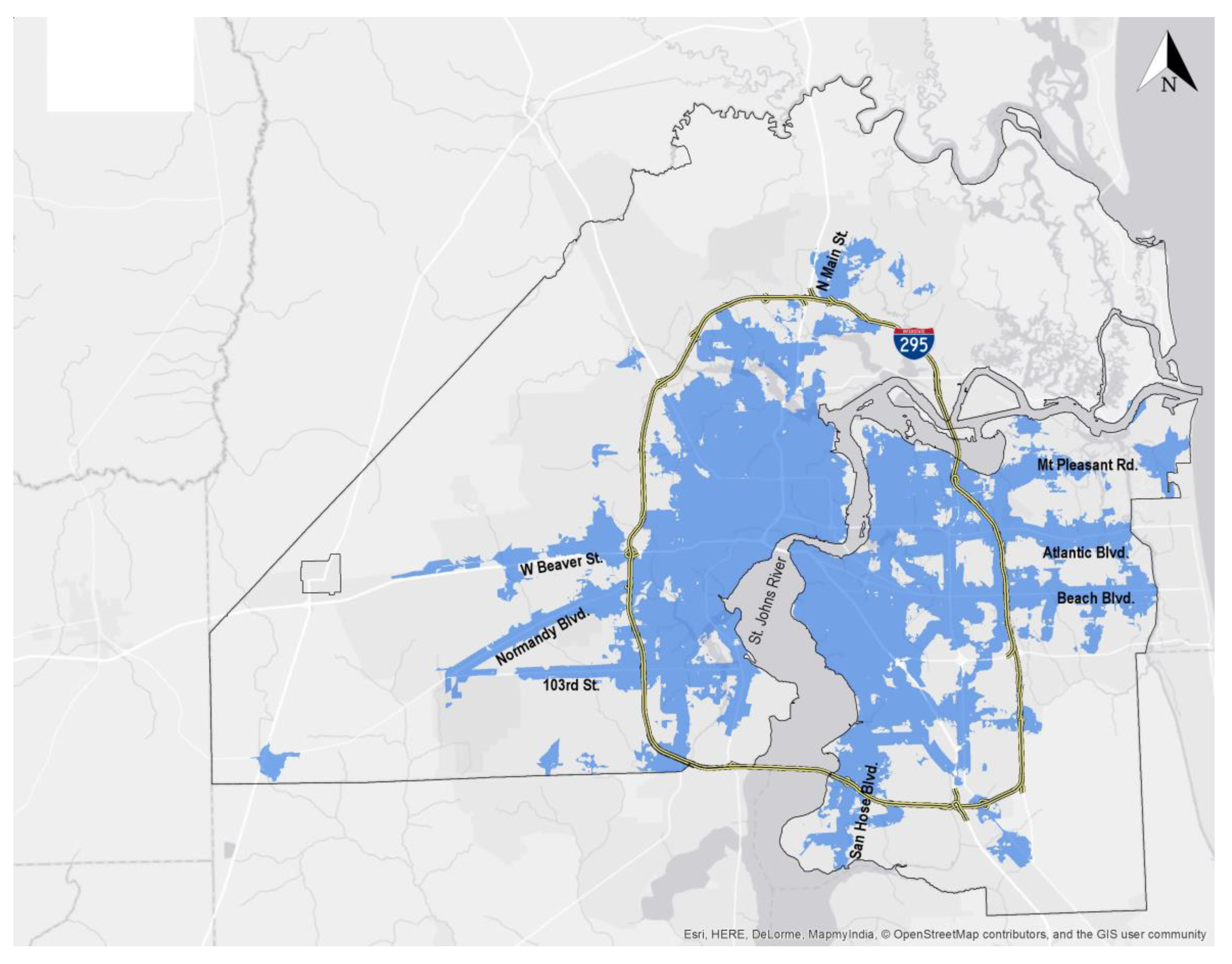
3.1. GIS Modeling Results

Figure 2 presents the GIS modeling results. The map shows the scored cells, which are mainly between 3 and 6, as well as their spatial distributions. In descriptive statistics, this case ranges from 0.06 to 8.94 (M = 2.86, SD = 1.84). The distributions of active built environment index are skewed to the right since the mean is greater than the median (2.54). To distinguish the pattern, cells above upper quartile value, which is 4.06, are split. As shown in Figure 3, higher-scored cells—cell value above 4.06—are concentrated inside I-295 and partially stretch out along 103rd Street, Normandy Boulevard, West Beaver Street, North Main Street, Mt Pleasant Road, Atlantic Boulevard, Beach Boulevard, and San Hose Boulevard. The GIS modeling results reveal that the area inside I-295 contains more active built environment features than other areas.

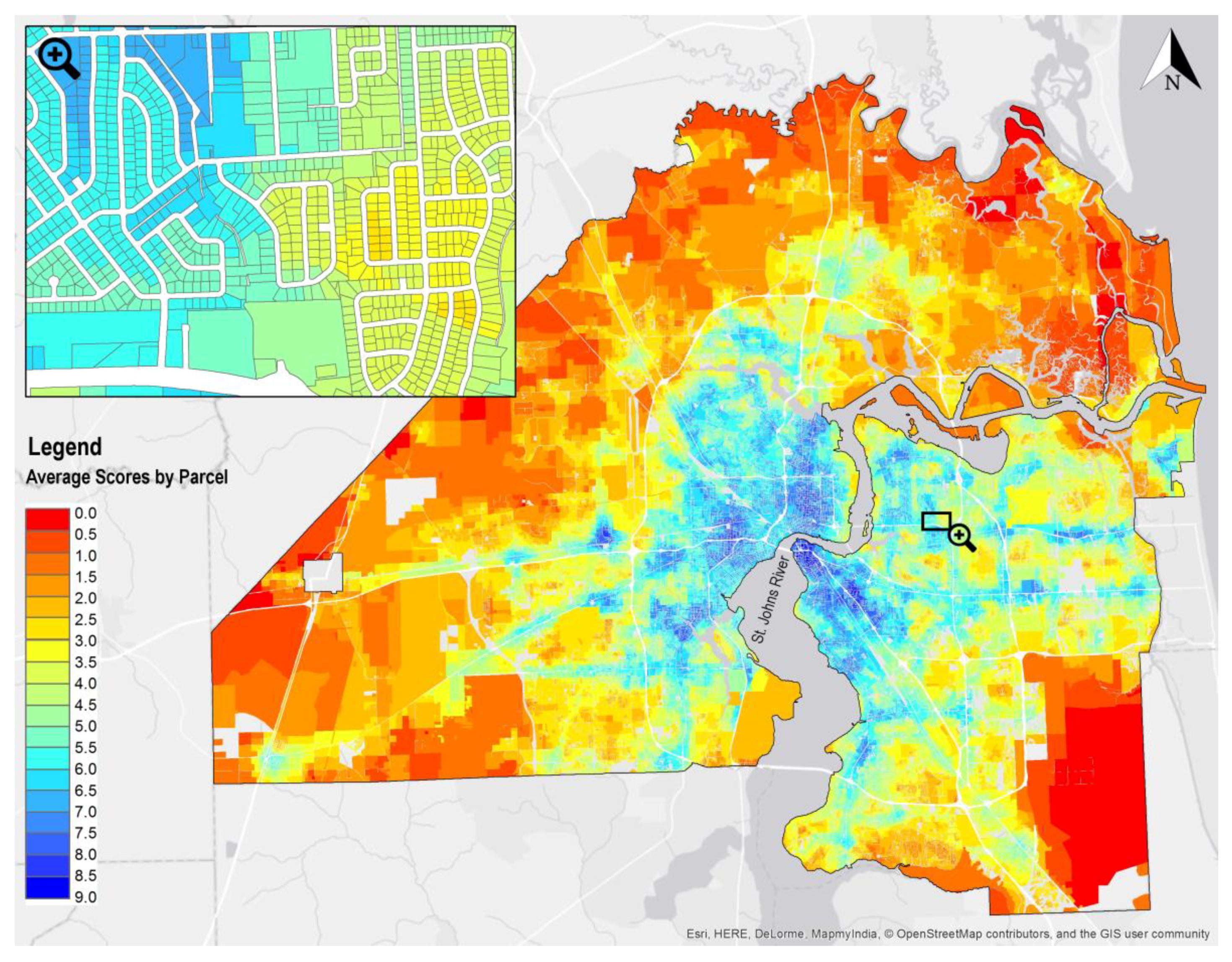
3.2. Applicaton of the GIS Modeling Results

The GIS modeling result demonstrates the indexed spatial pattern of active living potential by relevant geospatial dimensions. Using the zonal statistic function, the average value of the scored cells that belong to the parcel are computed. Figure 4 shows the average value of the cells for each parcel and their spatial patterns. In descriptive statistics, this case ranges from 0.28 to 8.85 (M = 4.53, SD = 1.54). Though the mean (4.53) and the median (4.50) are very close, the distributions of residential parcels’ scores are slightly skewed to the right since the mean is greater than the median.

3.2.1. Which Residential Types Have Higher (or Lower) Chances of Involving Physical Activity?

Since parcel data include detailed information regarding both residential types and scores, eight different residential types and their distributions of average scores are utilized (see Table 1). Jacksonville mainly consists of single-family parcels (about 80% of 292,698 total residential parcels) followed by about 7% condominiums, 3% mobile homes, and 2% multifamily housing. The descriptive statistics in Table 1 reveal that single-family parcels have lower score distributions—considering mean, median, lower quartile, and upper quartile—than other residential types including condominium, multifamily, boarding home, retirement home, and cooperative home. Since the majority of Jacksonville’s residential type is single family, this implies that most residents in Jacksonville might live with fewer active living features. In addition to single-family parcels, vacant residential parcels impose possible issues with regard to active living potential. Even compared to single-family parcels, which have lower active living potential than other residential types, vacant parcels show lower mean and median than single-family parcels. If these vacant parcels are developed without any enhancing of existing active built environments, then future residents might have lower chances of achieving recommended physical activity. To overcome this issue, urban planning techniques, such as urban design guidelines for active living, may intervene to improve the possibility of future residents’ physical activity.

3.2.2. Which Residential Types Are Highly Clustered with Higher Opportunities for Active Living?

As shown in Figure 2 and Figure 3, areas inside I-295 and along major roads have more potential for active living. While Figure 4 shows a broad spatial pattern of parcels, another analysis is helpful in identifying statistically significant hot spots, cold spots, and spatial outliers. Using Anselin Local Moran’s I statistic of spatial association, the results distinguish between statistically significant clusters of high values (HH), clusters of low values (LL), outliers in which high values are surrounded primarily by low values (HL), and outliers in which low values are surrounded primarily by high values (LH) at the 95% confidence level [54]. Figure 5 illustrates the cluster and outlier results. Although parts of major roads are identified as areas with higher value at Figure 3 (except Mt Pleasant Road and Beach Boulevard), higher-scored areas (i.e., 103rd Street, Normandy Boulevard, West Beaver Street, North Main Street, Atlantic Boulevard, and San Hose Boulevard) are recognized as spatial outliers in which a high value is surrounded primarily by low values.
Table 2 shows cluster and outlier analysis by type of residential parcel. Excluding outliers and statistically insignificant results, 41% of single-family parcels are assessed as clustered lower value while about 38% of the parcels are assessed as clustered higher value. The vacant residential parcels indicate results similar to those shown by single-family parcels (about 37% of clustered higher value and 48% of clustered lower value). However, the multifamily parcels include about 81% of clustered higher value compared to only 10% clustered lower value. Using these results, policymakers and urban planners will be able to prioritize areas clustered with lower values to improve the active living potential of current and future residents.

4. Discussion

My a priori assumption is that higher active built environment index would be mostly in the central area of the city due to available destinations and street network. As expected, areas having more active living potential are found inside I-295. However, other higher index regions are also located along several streets not in the central areas since these streets are close to identified destinations (e.g., grocery stores, schools and recreational space) and active transportation modes (e.g., bus routes and sidewalk). Although these extended areas along the streets turn out mostly spatial outliers (see Figure 5), this could also imply that urban planning intervention, such as adding new parks, might aid residents to live in active built environments.
To objectively measure the ways in which built environment affects physical activity, this paper describes the development of a comprehensive active built environment index to include relevant GIS variables, which represent geospatial dimensions of active living potential. The cell-based results of suitability modeling could not only identify areas in which residents will most likely become involved in physical activity, but also pinpoint other areas to urban planners or public health professionals that need to be developed to increase a region’s conduciveness to physical activity. The Jacksonville case study demonstrates both GIS-based visualization results and a potential toolset that can be used by policymakers, urban planners, and public health professionals to support the physical activity of residents. That is, urban planners or public health professionals could use the visualized results from this study as a broad resource to enhance physical activity opportunities of the study area. In addition to visualizing the existing conditions, if the planning or design intervention happens, this model could simulate the visualized effect of new intervention. Also, although this study employed a static model—having only ten variables weighted the same—increasing the GIS capacity could support a more dynamic model that would be more responsive to variable or weight changes over time.
This study employs parcel-level data to determine the variables of active built environment from a considerable amount of related studies. However, with the modeling process, the destinations from parcel data are not perfectly matched with existing literature. For example, to identify grocery stores, parcels including supermarkets and neighborhood or community shopping centers are used. However, it is possible that small retail shops might serve as a neighborhood grocery store for a certain area. Although FDOR data show a certain level of details, since the data might not have actual functions of the parcel, it is possible that this standardized FDOR database misses some information.
Regarding the entropy index, though the entropy calculation is generally an acceptable method to calculate land use diversity, the arguments about the entropy method should be noted. First, it has been shown that associations between walking and land use mix depend on which land uses are included in the calculation of entropy scores [55]. Second, land use mix might not be a strong predictor of walking. A review study has shown that 2 out of 4 studies on land use mix (entropy) and walking for transport found non-significant associations between them [56]. Third, entropy scores may not be correctly calculated in terms of the denominator, which is count of land uses [57]. Although there are the arguments of calculating the land use diversity, a considerable study concluded that land use diversity has a positive association with physical activity [4,13,14,15,16,17].
Another measurement used in the GIS model is a proximity measure using raster surfaces. This measurement is close to accessibility measurement which typically computes an ease of access to available destinations using distances between origins and destinations as a core frame [58,59,60]. This approach is convenient and valuable since it can be easily associated with zone-based datasets such as census boundary or transportation analysis zone. However, it has been recognized that zone-based analysis has a modifiable areal unit problem (MAUP), which indicates that the specific boundaries such as census block, census block group, or zip code make an impact on the accessibility results [58,61]. In other words, even at the same parcel or census block, the accessibility might not be identical. Since aforementioned methodologies used zone-based analysis, they might have MAUP [41,42,43,44,45]. However, the cell-based method utilized in this study compensates for MAUP by use of controllable cell size. Since a 5-m cell was used as the unit of analysis, each cell value could apply to any level of geographic unit even at the parcel level. In the results section, it is demonstrated how the raster layer is applicable to other geographic units by using the average scores of parcels instead of using a single value by parcel.
However, there are several limitations to this study. First, this study uses only quantified data. Researchers have argued that qualitative variables such as safety, comfort (which could include speed of traffic or speed limits) and pleasurability might make an impact on walkability [62]. However, to apply these qualitative variables, it is necessary to examine a local context of the study areas since the significance of those qualitative variables might be different by the context. In future research, after thorough studies regarding the local conditions, these qualitative variables could be considered in the modeling process. Second, this study uses the same weights for the combined layers since this study focuses more on the development of the GIS tool to evaluate active built environment. However, typical suitability modeling uses weighted layers to allow each variable to affect the model differently. Thus, future research may consider establishing an appropriate weight for each variable. Finally, this study assesses built environment regarding physical activity potential. However, recent developments in smartphone and smartwatch technology are enabling researchers to analyze the actual movements of people [63,64]. Therefore, in future research, tracking the movement patterns of residents via wearable smart devices would enable the examination of the relationships between actual physical activities and active living potential measures developed in this study. Such data would tremendously enhance the methodology adopted in this study.

Conflicts of Interest

The authors declare no conflict of interest.

References

  1. Centers for Disease Control and Prevention. Maps of Trends in Diabetes and Obesity. 2018. Available online: https://www.cdc.gov/diabetes/statistics/slides/maps_diabetesobesity_trends.pptx (accessed on 28 May 2018).
  2. Eckel, R.H.; Kahn, S.E.; Ferrannini, E.; Goldfine, A.B.; Nathan, D.M.; Schwartz, M.W.; Smith, R.J.; Smith, S.R. Obesity and Type 2 Diabetes: What can be unified and what needs to be individualized? Diabetes Care 2011, 34, 1424–1430. [Google Scholar] [CrossRef] [PubMed] [Green Version]
  3. Sullivan, P.W.; Morrato, E.H.; Ghushchyan, V.; Wyatt, H.R.; Hill, J.O. Obesity, Inactivity, and the Prevalence of Diabetes and Diabetes-Related Cardiovascular Comorbidities in the U.S., 2000–2002. Diabetes Care 2005, 28, 1599–1603. [Google Scholar] [CrossRef] [PubMed]
  4. Aytur, S.A.; Rodriguez, D.A.; Evenson, K.R.; Catellier, D.J.; Rosamond, W.D. Promoting Active Community Environments Through Land Use and Transportation Planning. Am. J. Health Promot. 2007, 21, 397–407. [Google Scholar] [CrossRef] [PubMed]
  5. Frank, L.; Kerr, J.; Chapman, J.; Sallis, J. Urban form relationships with walk trip frequency and distance among youth. Am. J. Health Promot. 2007, 21, 305–311. [Google Scholar] [CrossRef] [PubMed]
  6. Cohen, D.A.; Sehgal, A.; Williamson, S.; Golinelli, D.; Lurie, N.; McKenzie, T.L. Contribution of Public Parks to Physical Activity. Am. J. Public Health 2007, 97, 509–514. [Google Scholar] [CrossRef] [PubMed]
  7. Handy, S.L.; Xinyu, C.; Mokhtarian, P.L. The Causal Influence of Neighborhood Design on Physical Activity within the Neighborhood: Evidence from Northern California. Am. J. Health Promot. 2008, 22, 350–358. [Google Scholar] [CrossRef] [PubMed]
  8. Kaczynski, A.T.; Potwarka, L.R.; Saelens, B.E. Association of Park Size, Distance, and Features with Physical Activity in Neighborhood Parks. Am. J. Public Health 2008, 98, 1451–1456. [Google Scholar] [CrossRef] [PubMed]
  9. Lopez-Zetina, J.; Lee, H.; Friis, R. The link between obesity and the built environment. Evidence from an ecological analysis of obesity and vehicle miles of travel in California. Health Place 2006, 12, 656–664. [Google Scholar] [CrossRef] [PubMed]
  10. Sturm, R.; Cohen, D.A. Suburban sprawl and physical and mental health. Public Health 2004, 118, 488–496. [Google Scholar] [CrossRef] [PubMed]
  11. Squires, G.D. Urban Sprawl: Causes, Consequences, & Policy Responses; Urban Institute Press: Washington, DC, USA, 2002. [Google Scholar]
  12. Lopez, R.P.; Hynes, H.P. Obesity, physical activity, and the urban environment: Public health research needs. Environ. Health 2006, 5, 25. [Google Scholar] [CrossRef] [PubMed] [Green Version]
  13. City of New York. Active Design Guidelines: Promoting Physical Activity and Health in Design. 2010; pp. 1–135. Available online: https://www1.nyc.gov/assets/planning/download/pdf/plans-studies/active-design-guidelines/adguidelines.pdf (accessed on 28 May 2018).
  14. Frank, L.D.; Andresen, M.A.; Schmid, T.L. Obesity relationships with community design, physical activity, and time spent in cars. Am. J. Prev. Med. 2006, 27, 87–96. [Google Scholar] [CrossRef] [PubMed]
  15. Frank, L.D.; Sallis, J.F.; Conway, T.L.; Chapman, J.E.; Saelens, B.E.; Bachman, W. Many Pathways from Land Use to Health. J. Am. Plan. Assoc. 2006, 72, 75–87. [Google Scholar] [CrossRef]
  16. Brownson, R.C.; Hoehner, C.M.; Day, K.; Forsyth, A.; Sallis, J.F. Measuring the Built Environment for Physical Activity: State of the Science. Am. J. Prev. Med. 2009, 36, S99–S123. [Google Scholar] [CrossRef] [PubMed]
  17. Mumford, K.G.; Contant, C.K.; Weissman, J.; Wolf, J.; Glanz, K. Changes in Physical Activity and Travel Behaviors in Residents of a Mixed-Use Development. Am. J. Prev. Med. 2011, 41, 504–507. [Google Scholar] [CrossRef] [PubMed]
  18. Morland, K.; Wing, S.; Diez Roux, A. The contextual effect of the local food environment on residents’ diets: The atherosclerosis risk in communities study. Am. J. Public Health 2002, 92, 1761–1767. [Google Scholar] [CrossRef] [PubMed]
  19. Sallis, J.F.; Glanz, K. Physical Activity and Food Environments: Solutions to the Obesity Epidemic. Milbank Q. 2009, 87, 123–154. [Google Scholar] [CrossRef] [PubMed]
  20. McDonald, N.C. Critical Factors for Active Transportation to School among Low-Income and Minority Students: Evidence from the 2001 National Household Travel Survey. Am. J. Prev. Med. 2008, 34, 341–344. [Google Scholar] [CrossRef] [PubMed]
  21. Babey, S.H.; Hastert, T.A.; Yu, H.; Brown, E.R. Physical Activity Among Adolescents: When Do Parks Matter? Am. J. Prev. Med. 2008, 34, 345–348. [Google Scholar] [CrossRef] [PubMed]
  22. Coutts, C. Greenway accessibility and physical-activity behavior. Environ. Plan. B Plan. Des. 2008, 35, 552–563. [Google Scholar] [CrossRef]
  23. Giles-Corti, B.; Broomhall, M.H.; Knuiman, M.; Collins, C.; Douglas, K.; Ng, K.; Lange, A.; Donovan, R.J. Increasing walking: How important is distance to, attractiveness, and size of public open space? Am. J. Prev. Med. 2005, 28, 169–176. [Google Scholar] [CrossRef] [PubMed]
  24. Moore, L.V.; Diez Roux, A.V.; Evenson, K.R.; McGinn, A.P.; Brines, S.J. Availability of Recreational Resources in Minority and Low Socioeconomic Status Areas. Am. J. Prev. Med. 2008, 34, 16–22. [Google Scholar] [CrossRef] [PubMed]
  25. Pierce, J.; Denison, A.; Arif, A.; Rohrer, J. Living near a trail is associated with increased odds of walking among patients using community clinics. J. Community Health 2006, 31, 289–302. [Google Scholar] [CrossRef] [PubMed]
  26. Rosenberg, D.E.; Sallis, J.F.; Conway, T.L.; Cain, K.L.; McKenzie, T.L. Active Transportation to School over 2 Years in Relation to Weight Status and Physical Activity. Obesity 2006, 14, 1771–1776. [Google Scholar] [CrossRef] [PubMed]
  27. Besser, L.M.; Dannenberg, A.L. Walking to Public Transit: Steps to Help Meet Physical Activity Recommendations. Am. J. Prev. Med. 2005, 29, 273–280. [Google Scholar] [CrossRef] [PubMed]
  28. Saelens, B.E.; Handy, S.L. Built Environment Correlates of Walking: A Review. Med. Sci. Sports Exerc. 2008, 40, S550–S566. [Google Scholar] [CrossRef] [PubMed]
  29. Roberts, J.D.; Rodkey, L.; Ray, R.; Saelens, B. Do Not Forget About Public Transportation: Analysis of the Association of Active Transportation to School among Washington, DC Area Children with Parental Perceived Built Environment Measures. J. Phys. Act. Health 2018, in press. [Google Scholar] [CrossRef] [PubMed]
  30. Boarnet, M.G.; Forsyth, A.; Day, K.; Oakes, J.M. The Street Level Built Environment and Physical Activity and Walking: Results of a Predictive Validity Study for the Irvine Minnesota Inventory. Environ. Behav. 2011, 43, 735–775. [Google Scholar] [CrossRef]
  31. Jacobs, J. The Death and Life of Great American Cities; Random House: New York, NY, USA, 1961. [Google Scholar]
  32. Cervero, R.; Kockelman, K. Travel demand and the 3Ds: Density, diversity, and design. Transp. Res. Part D 1997, 2, 199–219. [Google Scholar] [CrossRef]
  33. Chin, G.K.W.; Van Niel, K.P.; Giles-Corti, B.; Knuiman, M. Accessibility and connectivity in physical activity studies: The impact of missing pedestrian data. Prev. Med. 2008, 46, 41–45. [Google Scholar] [CrossRef] [PubMed]
  34. Eyler, A.A.; Brownson, R.C.; Bacak, S.J.; Housemann, R.A. The epidemiology of walking for physical activity in the United States. Med. Sci. Sports Exerc. 2003, 35, 1529–1536. [Google Scholar] [CrossRef] [PubMed]
  35. Frank, L.D.; Schmid, T.L.; Sallis, J.F.; Chapman, J.; Saelens, B.E. Linking objectively measured physical activity with objectively measured urban form: Findings from SMARTRAQ. Am. J. Prev. Med. 2005, 28, 117–125. [Google Scholar] [CrossRef] [PubMed]
  36. Gordon-Larsen, P.; Nelson, M.C.; Page, P.; Popkin, B.M. Inequality in the Built Environment Underlies Key Health Disparities in Physical Activity and Obesity. Pediatrics 2006, 117, 417–424. [Google Scholar] [CrossRef] [PubMed]
  37. King, D. Neighborhood and Individual Factors in Activity in Older Adults: Results from the Neighborhood and Senior Health Study. J. Aging Phys. Act. 2008, 16, 144–170. [Google Scholar] [CrossRef] [PubMed]
  38. Reed, J.A.; Wilson, D.K.; Ainsworth, B.E.; Bowles, H.; Mixon, G. Perceptions of Neighborhood Sidewalks on Walking and Physical Activity Patterns in a Southeastern Community in the US. J. Phys. Act. Health 2006, 3, 243–253. [Google Scholar] [CrossRef] [PubMed]
  39. Dill, J. Bicycling for Transportation and Health: The Role of Infrastructure. J. Public Health Policy 2009, 30, S95–S110. [Google Scholar] [CrossRef] [PubMed]
  40. Pucher, J.; Buehler, R. Making cycling irresistible: Lessons from the Netherlands, Denmark and Germany. Transp. Rev. 2008, 28, 495–528. [Google Scholar] [CrossRef]
  41. Duncan, D.T.; Aldstadt, J.; Whalen, J.; Melly, S.J.; Gortmaker, S.L. Validation of Walk Score® for Estimating Neighborhood Walkability: An Analysis of Four US Metropolitan Areas. Int. J. Environ. Res. Public Health 2011, 8, 4160–4179. [Google Scholar] [CrossRef] [PubMed]
  42. Chiu, M.; Shah, B.R.; Maclagan, L.C.; Rezai, M.; Austin, P.C.; Tu, J.V. Walk Score® and the prevalence of utilitarian walking and obesity among Ontario adults: A cross-sectional study. Health Rep. 2015, 26, 3–10. [Google Scholar] [PubMed]
  43. Witten, K.; Pearce, J.; Day, P. Neighbourhood Destination Accessibility Index: A GIS Tool for Measuring Infrastructure Support for Neighbourhood Physical Activity. Environ. Plan. A 2011, 43, 205–223. [Google Scholar] [CrossRef]
  44. Peiravian, F.; Derrible, S.; Ijaz, F. Development and application of the Pedestrian Environment Index (PEI). J. Transp. Geogr. 2014, 39, 73–84. [Google Scholar] [CrossRef]
  45. Glazier, R.H.; Creatore, M.I.; Weyman, J.T.; Fazli, G.; Matheson, F.I.; Gozdyra, P.; Moineddin, R.; Shriqui, V.K.; Booth, G.L. Density, Destinations or Both? A Comparison of Measures of Walkability in Relation to Transportation Behaviors, Obesity and Diabetes in Toronto, Canada. PLoS ONE 2014, 9, e85295. [Google Scholar] [CrossRef] [PubMed]
  46. Koohsari, M.J.; Owen, N.; Cerin, E.; Giles-Corti, B.; Sugiyama, T. Walkability and walking for transport: Characterizing the built environment using space syntax. Int. J. Behav. Nutr. Phys. Act. 2016, 13, 121. [Google Scholar] [CrossRef] [PubMed]
  47. Saelens, B.E.; Sallis, J.F.; Black, J.B.; Chen, D. Neighborhood-based differences in physical activity: An environment scale evaluation. Am. J. Public Health 2003, 93, 1552–1558. [Google Scholar] [CrossRef] [PubMed]
  48. Story, M.; Giles-Corti, B.; Yaroch, A.L.; Cummins, S.; Frank, L.D.; Huang, T.T.; Lewis, L.B. Work Group IV: Future Directions for Measures of the Food and Physical Activity Environments. Am. J. Prev. Med. 2009, 36, S182–S188. [Google Scholar] [CrossRef] [PubMed]
  49. Centers for Disease Control and Prevention. Diagnosed Diabetes Prevalence County Estimates. 2018. Available online: https://www.cdc.gov/diabetes/atlas/obesityrisk/dmprev_xls/Florida.xlsx (accessed on 28 May 2018).
  50. Carr, M.H.; Zwick, P.D. Smart Land-Use Analysis: The LUCIS Model Land-Use Conflict Identification Strategy; ESRI Press: Redlands, CA, USA, 2007. [Google Scholar]
  51. Manaugh, K.; Kreider, T. What is mixed use? Presenting an interaction method for measuring land use mix. J. Transp. Land Use 2013, 6, 63–72. [Google Scholar] [CrossRef]
  52. Mitchell, A. Modeling Suitability, Movement, and Interaction; ESRI Press: Redlands, CA, USA, 2012; Volume 3. [Google Scholar]
  53. Elaalem, M.; Comber, A.; Fisher, P. A Comparison of Fuzzy AHP and Ideal Point Methods for Evaluating Land Suitability. Trans. GIS 2011, 15, 329–346. [Google Scholar] [CrossRef]
  54. Environmental Systems Research Institute (ESRI). Cluster and Outlier Analysis (Anselin Local Moran’s I). 2018. Available online: http://pro.arcgis.com/en/pro-app/tool-reference/spatial-statistics/cluster-and-outlier-analysis-anselin-local-moran-s.htm (accessed on 28 May 2018).
  55. Christian, H.E.; Bull, F.C.; Middleton, N.J.; Knuiman, M.W.; Divitini, M.L.; Hooper, P.; Amarasinghe, A.; Giles-Corti, B. How important is the land use mix measure in understanding walking behaviour? Results from the RESIDE study. Int. J. Behav. Nutr. Phys. Act. 2011, 8. [Google Scholar] [CrossRef] [PubMed]
  56. Grasser, G.; Stronegger, W.; Titze, S.; Van Dyck, D. Objectively measured walkability and active transport and weight-related outcomes in adults: A systematic review. Int. J. Public Health 2013, 58, 615–625. [Google Scholar] [CrossRef] [PubMed]
  57. Hajna, S.; Dasgupta, K.; Joseph, L.; Ross, N.A. A call for caution and transparency in the calculation of land use mix: Measurement bias in the estimation of associations between land use mix and physical activity. Health Place 2014, 29, 79–83. [Google Scholar] [CrossRef] [PubMed]
  58. Handy, S.L.; Niemeier, D.A. Measuring accessibility: An exploration of issues and alternatives. Environ. Plan. A 1997, 29, 1175–1194. [Google Scholar] [CrossRef]
  59. Hansen, W.G. How Accessibility Shapes Land Use. J. Am. Inst. Plan. 1959, 25, 73–76. [Google Scholar] [CrossRef]
  60. Miller, H.J. Place-Based versus People-Based Accessibility. Access to Destinations; Levinson, D.M., Krizek, K.J., Eds.; Emerald Group Publishing Limited: Bingley, UK, 2005; pp. 63–89. [Google Scholar]
  61. Neutens, T.; Versichele, M.; Schwanen, T. Arranging place and time: A GIS toolkit to assess person-based accessibility of urban opportunities. Appl. Geogr. 2010, 30, 561–575. [Google Scholar] [CrossRef]
  62. Ewing, R.; Handy, S. Measuring the Unmeasurable: Urban Design Qualities Related to Walkability. J. Urban Des. 2009, 14, 65–84. [Google Scholar] [CrossRef]
  63. Piwek, L.; Joinson, A.; Morvan, J. The use of self-monitoring solutions amongst cyclists: An online survey and empirical study. Transp. Res. Part A Policy Pract. 2015, 77, 126–136. [Google Scholar] [CrossRef]
  64. Patel, M.S.; Foschini, L.; Kurtzman, G.W.; Zhu, J.; Wang, W.; Rareshide, C.A.L.; Zbikowski, S.M.; Zhu, J.; Wang, W. Using Wearable Devices and Smartphones to Track Physical Activity: Initial Activation, Sustained Use, and Step Counts Across Sociodemographic Characteristics in a National Sample. Ann. Intern. Med. 2017, 167, 755–757. [Google Scholar] [CrossRef] [PubMed]
Figure 1. Conceptual framework of this study.
Urbansci 02 00044 g001
Figure 2. GIS modeling results ranked by active built environment index.
Urbansci 02 00044 g002
Figure 3. Highlighted cells above value above upper quartile.
Urbansci 02 00044 g003
Figure 4. Average scores by parcel.
Urbansci 02 00044 g004
Figure 5. Cluster & outlier analysis of scored parcel.
Urbansci 02 00044 g005
Table 1. Distributions of average scores by residential parcel type.
Residential TypeNumber of Parcels (%)Descriptive Statistics *
MMdnLQUQMinMaxSD
Single Family234,844 (80.23%)4.5544.4873.3165.7930.2948.8411.504
Condominium21,420 (7.32%)4.8694.8363.6285.7432.1958.6231.262
Multifamily5127 (1.75%)6.0876.3675.6037.0170.2828.8491.398
Mobile Home9648 (3.30%)3.5283.3162.4674.4650.2998.4511.382
Boarding Home8 (0.00%)6.4827.1406.4667.4092.0437.7821.876
Retirement Home24 (0.01%)5.2895.1703.9446.5752.5247.4621.457
Cooperative121 (0.04%)7.2937.2747.2457.2747.1577.7450.119
Vacant Residential21,506 (7.35%)4.3694.2072.7535.9420.2988.5191.767
Grand Total292,698 (100.00%)4.5534.5013.2865.8030.2828.8491.535
* M: Mean; Mdn: Median; LQ: Lower Quartile; UP: Upper Quartile; Min: Minimum; Max: Maximum; SD: Standard Deviation.
Table 2. Cluster and outlier analysis by residential parcel type.
Residential TypeTotal Number of ParcelsNumber of Parcels by Cluster & Outlier Type *
HHHLLHLLNS
Single Family234,844 (100%)89,711 (38.20%)3501 (1.49%)8731 (3.72%)96,693 (41.17%)36,208 (15.42%)
Condominium21,420 (100%)5920 (27.64%)39 (0.18%)116 (0.54%)5303 (24.76%)10,042 (46.88%)
Multifamily5127 (100%)4132 (80.59%)87 (1.70%)66 (1.29%)534 (10.42%)308 (6.00%)
Mobile Home9648 (100%)1230 (12.75%)328 (3.40%)109 (1.13%)6601 (68.42%)1380 (14.30%)
Boarding Home8 (100%)7 (87.50%)--1 (12.50%)-
Retirement Home24 (100%)11 (45.83%)3 (12.50%)-6 (25.00%)4 (16.67%)
Cooperative121 (100%)121 (100.00%)----
Vacant Residential21,506 (100%)7996 (37.18%)306 (1.42%)415 (1.93%)10,206 (47.46%)2539 (12.01%)
Grand Total292,698 (100%)109,128 (37.28%)4264 (1.46%)9437 (3.23%)119,344 (40.77%)50,525 (17.26%)
* HH: Cluster of High values; HL: High value surrounded by Low value (Outlier); LH: Low value surrounded by High value (Outlier); LL: Cluster of Low values; NS: Not Significant.

