Abstract
Submarines are required to have good performance, which is influenced by their type of hull, hull conditions, and operational conditions. This study compares the resistance between a Modified-U209 (U209) submarine and the DARPA Suboff. The former is an older hull geometry with both surface and submerged operation considered, whereas the latter represents a modern nuclear-powered submarine designed for submerged operations only. The two geometries were scaled to give the same usable volume, and all results were non-dimensionalized using this to ensure consistency. A Computational Fluid Dynamics (CFD) method was utilized to predict resistance by employing the Reynolds-averaged Navier–Stokes (RANS) equations. The results show that the total resistance coefficient for the U209 bare hull is approximately 6% higher than the Suboff bare hull. When a casing was added to the U209 geometry the increase in total resistance coefficient was approximately 8%. The addition of the sail resulted in an increase in total resistance coefficient ranging from approximately 4% (Suboff sail added to U209) to approximately 14% (U209 sail added to U209). An existing empirical prediction technique was used to predict the resistance, with the total resistance coefficient predicted being consistently about 5% lower than the values obtained using CFD.
1. Introduction
1.1. Background
Submarines have played a crucial role in naval warfare and strategic defense for decades. Their unique ability to operate underwater, hidden from adversaries, gives them a distinct advantage in reconnaissance, surveillance and covert operations [1]. Their military importance around the world is continuing to grow, with many navies modernizing and increasing the size of their submarine fleets [2].
Submarines are an effective tool in both anti-ship and anti-submarine warfare due to their stealth and surprise tactics [3,4]. Their ability to remain undetected underwater allows them to gather intelligence, track enemy movements and launch attacks with precision. Furthermore, submarines are highly effective in hit-and-run attacks, attrition warfare and single salvo strikes ashore. They excel in missions that require quick strikes and minimal exposure, making them invaluable assets for disrupting enemy supply lines and executing targeted campaigns [5].
Submarines are also crucial for strategic nuclear deterrence, providing a second-strike capability in the event of a nuclear exchange. Their ability to carry and launch nuclear armed ballistic missiles from hidden locations beneath the ocean’s surface makes them a key component of national security strategies for many countries. Because of this, attack submarines are also used extensively to track enemy ballistic missile capable submarines, such that they can be neutralized prior to launching their ballistic missiles in the event of the outbreak of hostilities.
In addition to their military applications, submarines also play a vital role in scientific research and exploration of the ocean depths. Their manned and unmanned missions have led to groundbreaking discoveries and enhanced the understanding of the mysteries hidden beneath the sea. They are vital for studying and documenting marine life, geological formations and hydrothermal vents in the deep ocean [6].
Submarines have evolved from surface ships that are able to submerge from time to time, for example to evade detection or to attack a surface ship (better described as “submersibles”), to those designed to remain submerged throughout their whole mission: the true submarine. As the latter are not required to operate on the surface of the ocean, their hull shapes are quite different from those of the former.
Research into submarine hydrodynamic performance is generally very classified, and it is not possible to publish results without giving away details of a nation’s submarine designs. To assist in conducting submarine hydrodynamics research that could be shared in the public domain, the submarine technology office of the Defense Advanced Research Projects Agency (DARPA) in the US, developed an unclassified submarine shape, referred to as Suboff [7,8]. It was intended that this represents a typical modern (at the time) large nuclear-powered attack submarine—a true submarine. This has been used by many researchers in the field.
Renilson [9] summarized much of the work in this field, and presented detailed information about the geometry of the Suboff. Zheku et al. [10] used the Suboff geometry to assess numerical approaches to captive model tests. Uzen et al. [11] and Utama et al. [12] used the Suboff geometry to study the influence of biofouling on the drag of a submarine. Lyu et al. [13] used the Suboff geometry to investigate microbubble resistance reduction. Kinaci et al. [14] used the Suboff geometry to investigate self-propulsion using CFD and made comparisons with empirical methods. Chase and Carrica [15] used the DARPA Suboff and its propeller E1619 to investigate different turbulence modeling approaches. Byeon et al. [16] also used the DARPA Suboff geometry and propeller E1619 to simulate self-propulsion and investigate the wake velocities behind the submarine. They reported good agreement with experimental results. Delen and Kinaci [17] used the DARPA Suboff model to conduct direct CFD simulations of maneuvering tests.
The small diesel–electric 209 type of submarine (U209) was developed by Howaldtswerke-Deutsche Werft (HDW) in the late 1960s. This was based on type 206 and is generally considered a derivative of wartime designs, whose hull forms are compromises between surface and sub-surface performance. There are many varieties of type 209, with some still being used by a number of nations, including Indonesia. The geometry of the U209 is given in [18].
The design philosophies for these two submarines are quite different. Type 209 is a lot older, and designed with operations on the surface, as well as submerged, in mind. On the other hand, the Suboff is a more modern form with an axisymmetric hull, meant to represent a nuclear-powered submarine, designed purely for operations submerged. Nuclear submarines only spend very limited time on the surface.
1.2. Aim of Present Work
The main aim of the present work is to investigate the influence of geometry, including casing and sail, on the resistance of a submarine. Two basis submarines are used: the DARPA Suboff geometry [7,8] and the U209 geometry [18]. Sufficient details are available in the public domain for both geometries to enable such calculations to be carried out.
In order to make a meaningful comparison between these two geometries their dimensions were scaled to give them both the same usable volume, defined as the same volume in the hull, excluding the casing and the sail. The principal dimensions of the resulting submarines are given in Table 1. Note that these are all at model scale to make comparison with experimental results easier. However, the trends in the results will apply to a full-scale submarine, regardless of the size.

Table 1.
Principal particulars of all cases.
L is the overall length of the submarine; D is the diameter of the pressure hull; Lpmb is the length of the parallel middle body; S is the total wetted surface area (including casing and sail, where relevant); and ∇ is the total volume (including casing and sail, where relevant). The greater values of S and ∇ for Cases 3–6 compared to Cases 1 and 2 reflects the increase in wetted surface area and volume due to the casing and sail. As these will be free flood spaces, they are not considered to increase the useable volume of the submarine. In each case, the usable volume was kept constant at 0.755m3.
Schematics of the geometries of the six cases are given in Figure 1.
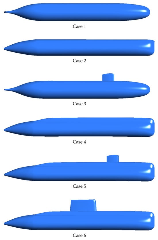
Figure 1.
Schematic of the six cases studied.
Note that as the Suboff was developed to represent a large nuclear-powered submarine it was designed to operate below the surface only. However, U209 was designed with surface, as well as submerged, operations in mind. Hence, U209 has a different bow shape, and a greater value of L/D than the Suboff. Both these characteristics would suggest that U209 will have a greater resistance when submerged than the Suboff. In addition, the Suboff has no casing, and only a small sail (relative to the size of the hull) whereas U209 has both a casing and a large sail. Again, both these characteristics would suggest that U209 will have a greater resistance.
It is interesting to note that despite the differences in the shapes of the two bare hulls (Case 1 and Case 2), as shown in the schematic diagrams in Figure 2, they have very similar wetted surface areas. An empirical estimation of the wetted surface of a submarine hull, knowing only its diameter, length, and length of parallel middle body was developed by one of the authors [9] and is given in Equation (1).

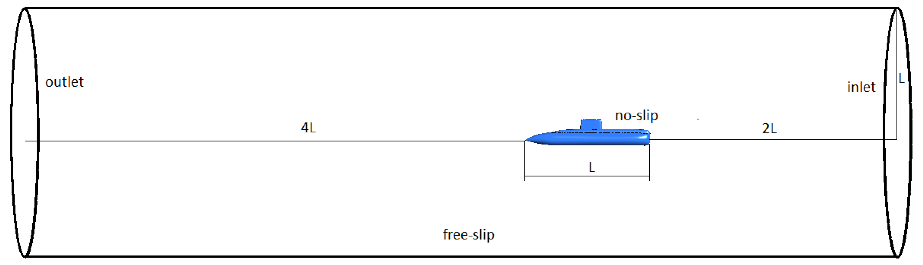
Figure 2.
Computational Domain.
Using Equation (1) the wetted surface of the hull alone can be estimated for both cases. These are compared with the measured values in Table 2. The estimate of the wetted surface using Equation (1) for the Suboff is very good, being only 0.41% higher than the actual value. The estimate of the wetted surface using Equation (1) for U209 is not so good, being about 3% too low. However, considering that the hull shape of U209 is quite different to the data used to generate Equation (1), this is still remarkably close. Thus, it is possible to conclude that Equation (1) gives a very good estimate of the wetted surface of a submarine hull (without casing), suitable for the early design stage.
Table 2.
Wetted surface area of bare hull cases.
As can be seen from Table 1, in order to achieve the same usable volume, the two geometries had different overall lengths, and wetted surfaces, so to make the results consistent the drag was non-dimensionalized using the usable volume, C∇, as given in Equation (2).
where R is the drag of the submarine; ρ is the water density; V is the speed of the submarine, and ∇u is the usable volume.
In addition, as the two geometries have different lengths for the same usable volume, to compare the results using the Reynolds number based on length would be inconsistent. Hence, for this study, the Reynolds number was based on volume, Re∇, as given in Equation (3).
where ν is the kinematic viscosity of the water.
2. Method
The investigation was carried out using Computational fluid dynamics (CFD) as a tool for resistance estimation as discussed below. This has been used before by the authors for this purpose [12].
2.1. Background
CFD using the Reynolds-averaged Navier–Stokes (RANS) approach has been used successfully to make predictions of the drag of a ship for many years [19,20,21,22,23]. For this work the implementation of RANS within ANSYS-CFX was utilized. ANSYS 2023 R2 version, developed by ANSYS, Inc., based in Canonsburg, Pennsylvania, USA, is used in this case.
It has been shown that the selection of turbulence models is of most importance as applied to the modeling of wake fields. The k-e turbulence model was used for this work. The k-e turbulence model has been widely used in industrial applications and research because it is relatively economical in terms of CPU time, especially when compared to models like the SST turbulence model [24,25,26,27,28].
It is noted, however, that Byeon et al. [16] compared the predicted results using CFD obtained with various turbulence models to experimental results for a fully appended DARPA Suboff model. They found that for this case, the Reynolds stress turbulence model (RSM) showed the best agreement with the experimental results, although it is worth noting that they appeared to use smaller grid sizes than used in the current study, and that their work was on a fully appended hull form, with aft control surfaces, whereas the aft control surfaces were omitted in the current work to better demonstrate the difference due to hull form and sail configuration.
Park and Seok [29] used the k-ω SST to predict the drag on a fully appended model of the BB2 submarine, with and without mounting struts using a grid size of approximately 2 M. They also reported the total resistance coefficients predicted by six other national research organisations.
Mai et al. [30] used the k-ω SST to predict the hydrodynamic derivatives of a fully appended BB2 submarine. They conducted a grid convergence study for the static drift case with y+ = 1. They determined that a grid size of about 3M is appropriate for oblique motion, using the grid convergence index (CGI) method of Roache [31].
2.2. Modeling
The fluid flow field is solved with the help of the RANS solver, which is a component of ANSYS-CFX; Equation (4) and Equation (5), respectively.
In Equation (4), ρ is fluid density, t is time, and Uj is the flow velocity vector field.
The left side of the RANS equation (Equation (5)) represents the change in the mean momentum of the fluid element to the unsteadiness in the mean flow. This change is balanced by the mean body force (), the mean pressure field (), the viscous stress,, and apparent stress () to the fluctuating velocity field.
The ANSYS-CFX program utilizes a spatial discretization technique known as element-based finite volume, which is complemented by the implementation of a high-resolution strategy to stabilize the convective term. The process of time discretization is accomplished by the utilization of the Second Order Backward Euler scheme. The ANSYS-CFX software, 2023 R2 version, employs a linked solver that effectively solves the hydrodynamic equations, encompassing the variables of velocity components (u, v, w) and pressure (p) as a unified system. Initially, the non-linear equations undergo a process known as linearization using coefficients of iteration. Subsequently, the resulting linear equations are resolved using an Algebraic Multigrid (AMG) solver [32]. The convergence criterion utilized in both codes was established by assessing the residual error in the mass and momentum equations with a predetermined threshold of 10−4 [33,34] as discussed by Roache [31].
2.3. Domain
The computational domain used is a cylinder shown in Figure 2. It comprises a velocity inlet 2L forward of the submarine and an outlet 5L aft of the submarine. The radius of the domain is L.
The boundary of the domain is defined as a free-slip condition, and the surface of the hull is defined as a fixed boundary with a no-slip condition. The domain size and the boundary conditions are shown in Figure 2.
The inlet flow velocity is prescribed, and the outlet hydrostatic pressure is defined as a function of water level.
2.4. Grid Convergence Independence
In this study, the DesignModeller in ANSYS-CFX was utilized to generate the mesh. Both structured and unstructured meshes were employed to decompose the computational domain. Due to the complex geometry of the hull, a mesh with triangular elements was constructed on its surface. Subsequently, the boundary layer was refined with prism elements by extending the surface mesh nodes. By strategically incorporating inflated tetrahedral elements proximate to the hull and employing an unstructured mesh in the distal region, we have markedly optimized the design. This approach not only enhances structural integrity but also significantly reduces the number of elements required, thereby increasing efficiency and performance. Such innovative techniques are essential for advancing engineering solutions and achieving favorable outcomes (as illustrated in Figure 3).
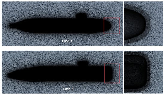
Figure 3.
Side view of hybrid mesh.
A fine mesh may always deliver reliable results in CFD, but at the same time, a finer mesh increases the computational cost and time consumption owing to the huge numbers of elements. The mesh size plays a significant part in the calculation operation.
Three mesh sizes were used for each case, for all four speeds. These ranged from 6,362,594 to 42,722,071 depending on the complexity of the geometry. Other than for the three lower speeds for Case 1, these all showed asymptotic convergence with Ri < 1.0 and GCI > 1.0. Hence, the finest mesh was used for the results given in this paper.
2.5. Turbulence Model Study
The selection of an appropriate turbulence model is crucial in accurately determining ship resistance, particularly for vessels where frictional resistance is the dominant component, as in this case, where the ship operates at a low speed (low Reynolds number). To identify the most suitable turbulence model, this study conducted a turbulence model analysis, incorporating the turbulence model of k-ε with y+ = 150, k-ω with y+ = 0.5, and k-ω SST with y+ = 0.5.
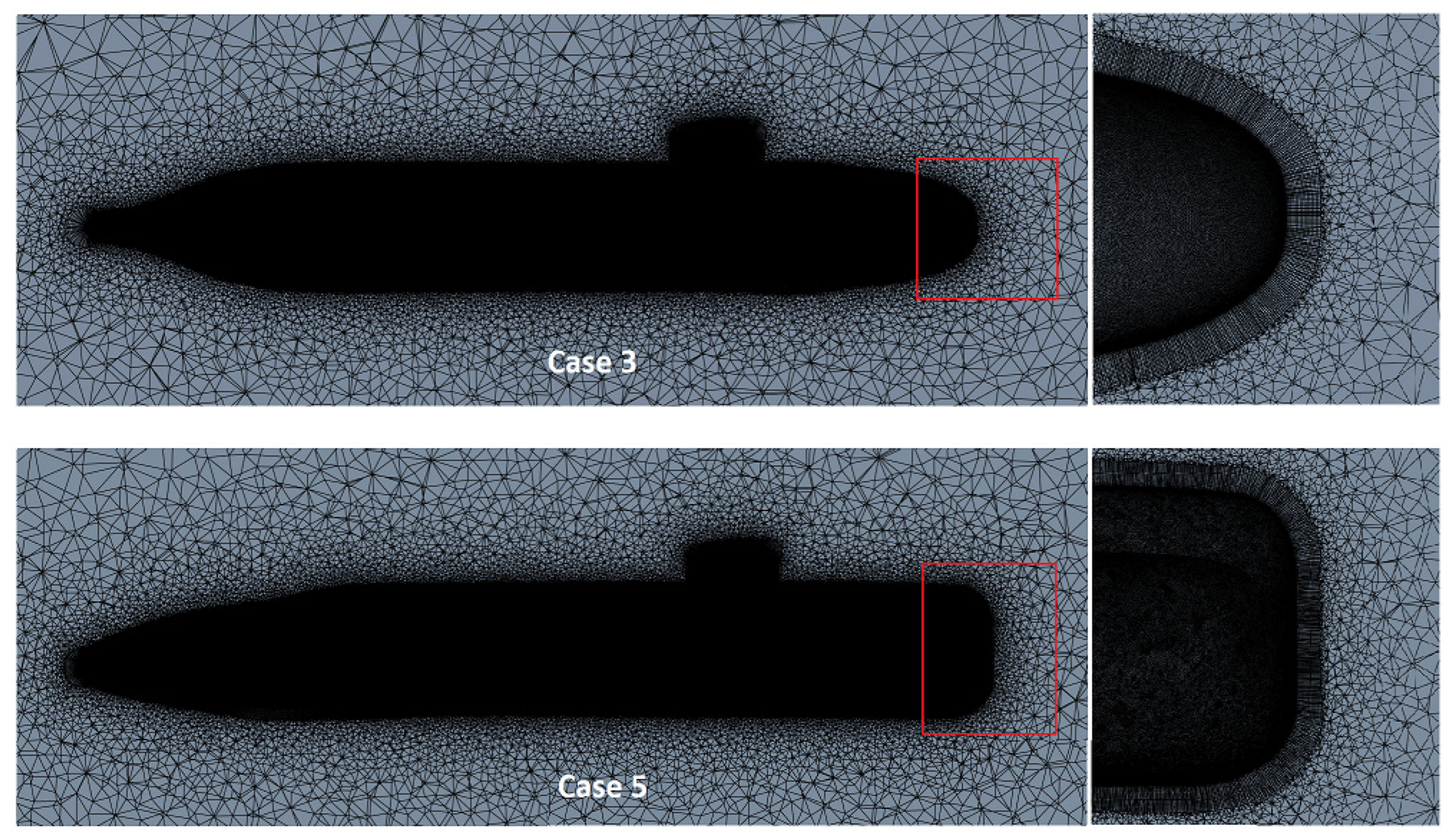
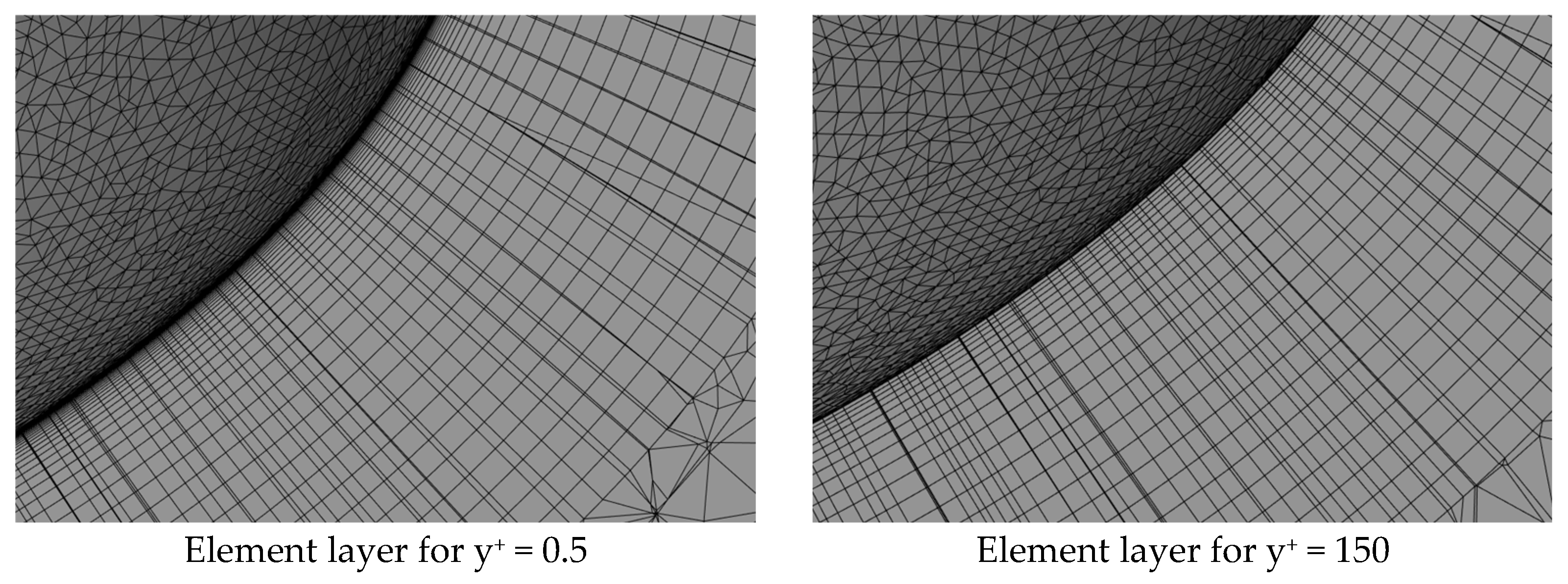
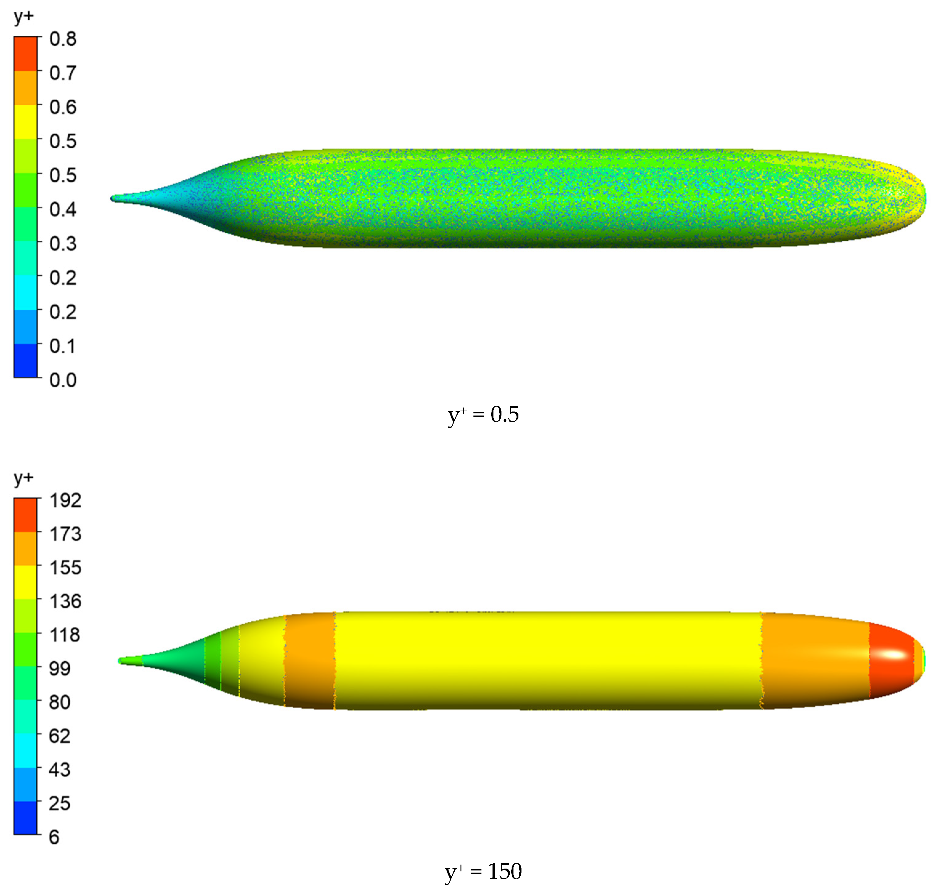
To achieve the targeted y+ values, adjustments were made to the number of element layers near the submarine surface and the height of the first-layer element. For y+ = 150, at a speed of 13.92 knots, 22 layers were used, with a first-layer height of 5.9 × 10⁻⁴. In contrast, for y+ = 0.5, 54 layers were used, with a first-layer height of 1.69 × 10⁻⁶. The element shape and the y+ distribution can be seen in Figure 4 and Figure 5.
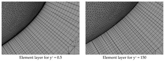
Figure 4.
Mesh near the submarine Case 1 (Suboff bare hull only) surface at speed 13.92 knots.
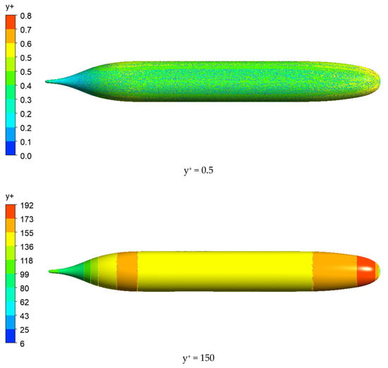
Figure 5.
Distribution of y+ of Case 1 (Suboff bare hull only) at speed 13.92 knots.
2.6. Validation Against Experimental Results
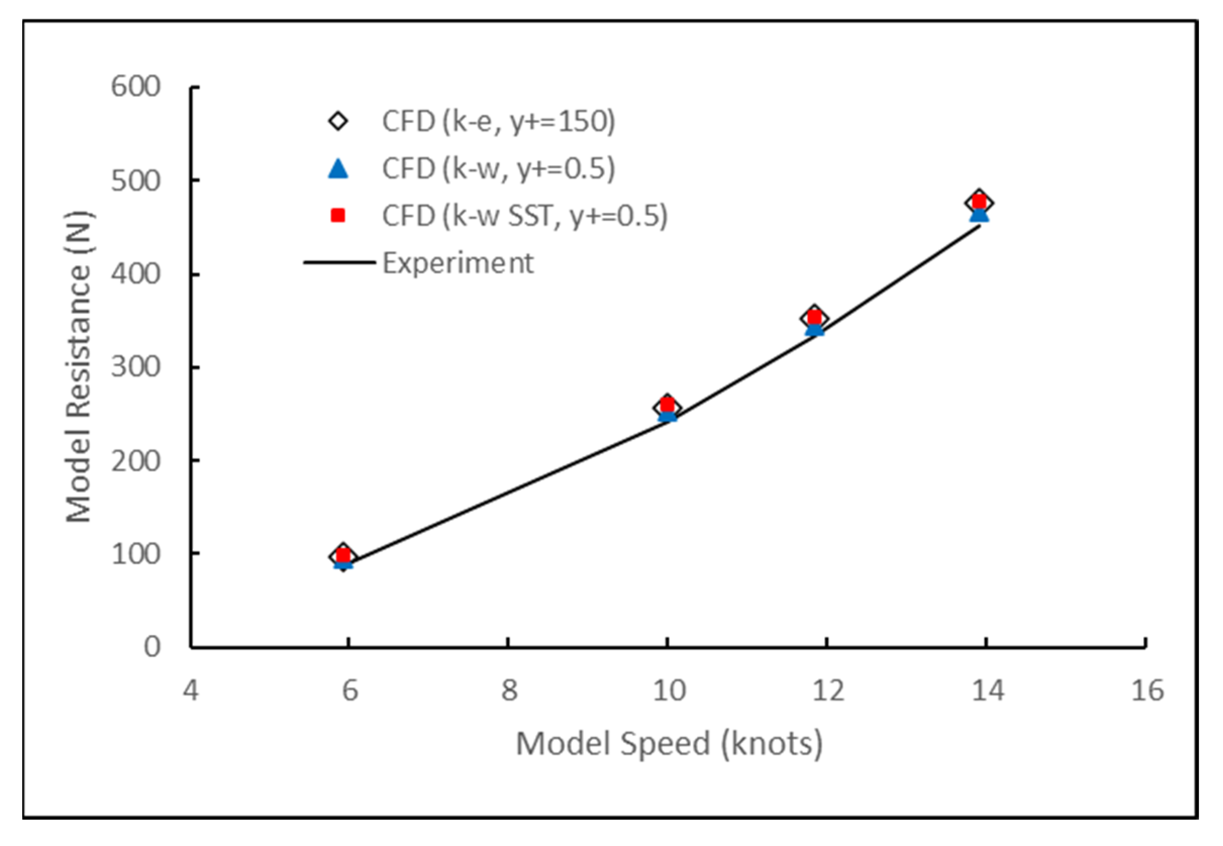
The method developed above was then applied to the Suboff geometry without a sail and the predictions compared with the experimentally measured results presented in [8]. The comparison is given in Figure 5.
As can be seen from Figure 6, there is generally very good agreement between the CFD predictions (for all turbulence models) and the measured results, which gave confidence in applying this approach to investigate the influence of geometry on resistance.
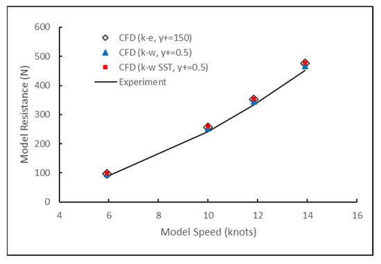
Figure 6.
Comparison of experimental results from [8] with CFD predictions using present method.
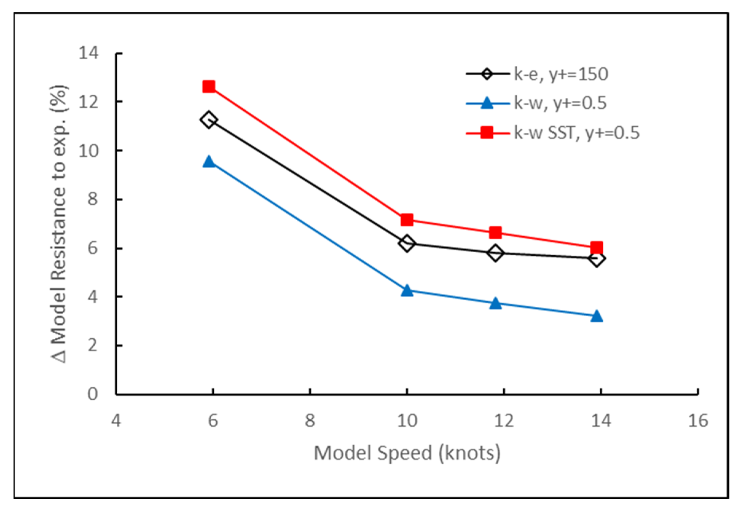
The percentage difference between each turbulence model and the experimental results (Figure 7) shows that the k-ω model yields the best results, with discrepancies ranging from 3.2% to 9.6% for speeds between 5.92 knots and 13.92 knots. In contrast, the k-ε turbulence model provides moderate results, with differences ranging from 5.6% to 11.3%. The k-ω SST turbulence model, however, produces the largest discrepancies among the three turbulence models, ranging from 6% to 12.6%.
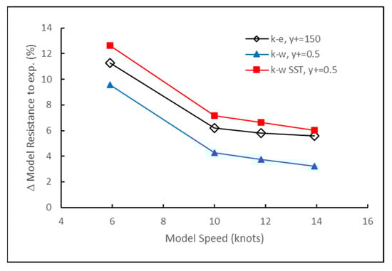
Figure 7.
The difference (in percentage) of model resistance between CFD and experiment.
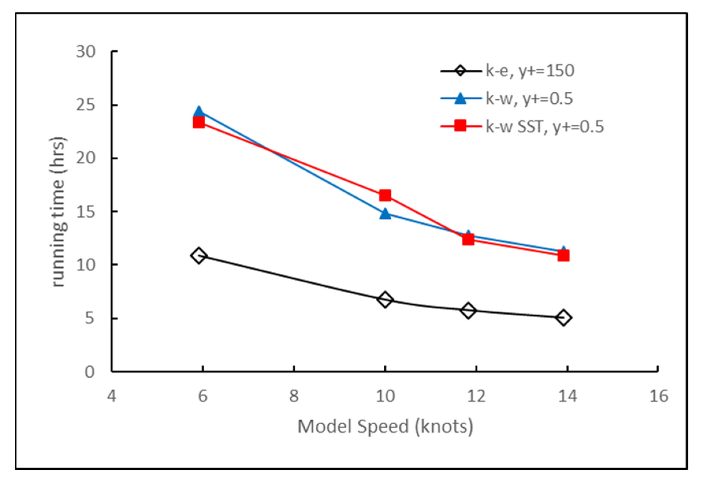
Regarding the running time (Figure 8), the k-ε turbulence model yields the best performance, with a lower running time ranging from 5 to 11 h. In contrast, the other turbulence models require running times between 11 and 25 h.
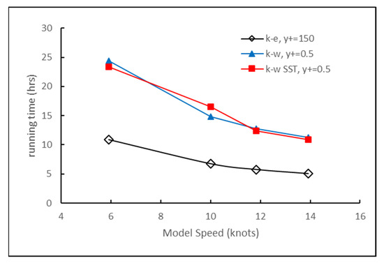
Figure 8.
The running time at different turbulence model.
The k-ε model should be more suitable for high Reynolds numbers, while the k-ω model is more appropriate for low Reynolds numbers, and the k-ω SST model is suitable for both. However, in this case, considering that the percentage differences from the experimental results are not significantly large between the k-ε, k-ω, and k-ω SST models, while the running time differences are quite significant, the k-ε turbulence model was selected for this study.
3. Results and Discussion
3.1. Influence of Hull Shape
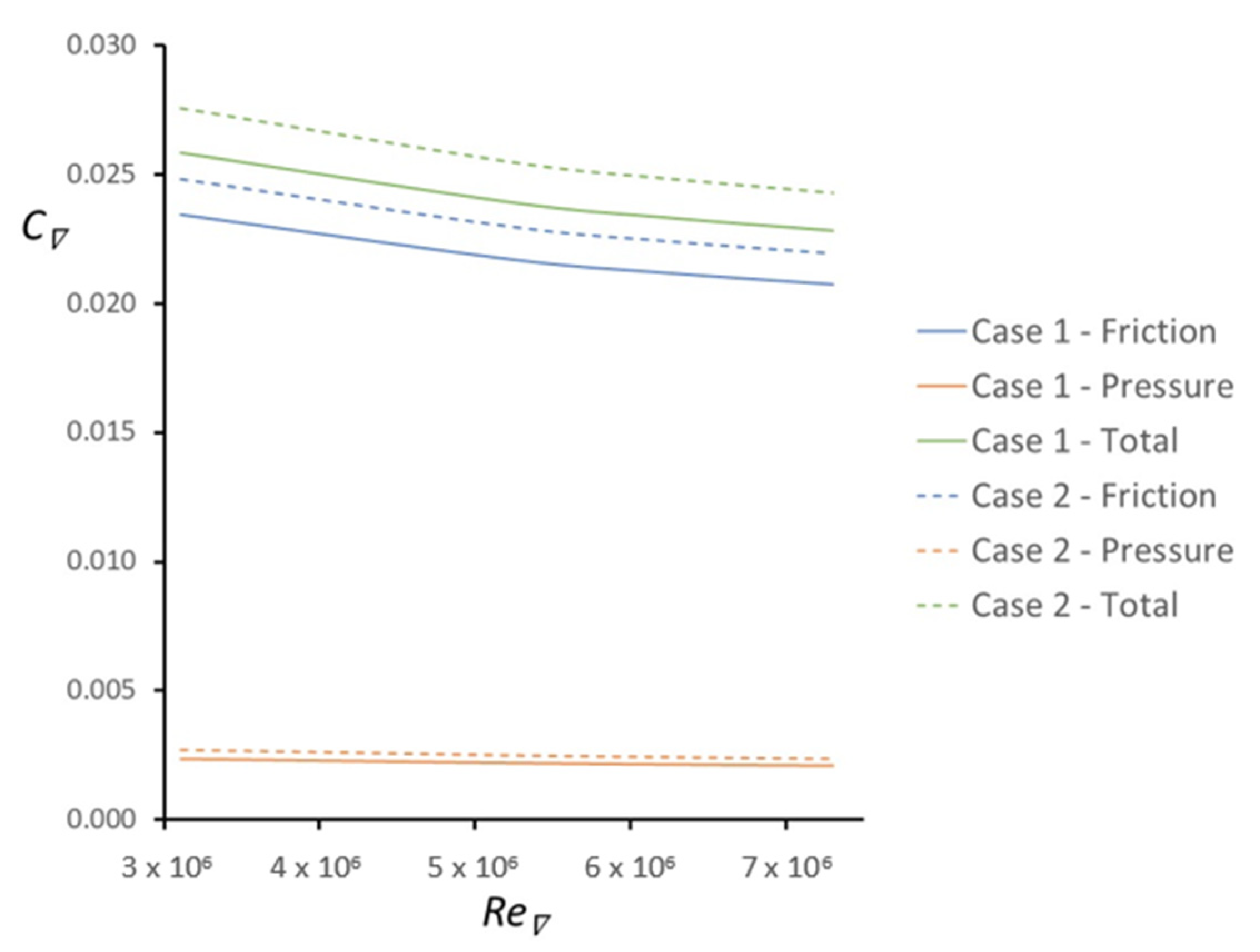
Figure 9 is a plot of the resistance coefficient, C∇, as a function of the Reynolds number, Re∇, for the two different bare hull geometries. Note that both have been non-dimensionalized using usable volume, as explained in Section 1.2. This presentation is consistent, and hence the results can be directly compared.
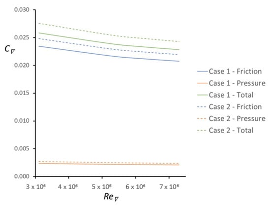
Figure 9.
Resistance coefficient as a function of Reynolds number for both bare hull cases (Case 1 = Suboff; Case 2 = U209).
As can be seen from Figure 9, the frictional resistance coefficient is about 5.7% greater for the U209 bare hull (Case 2) compared to the Suboff bare hull (Case 1). The U209 has an approximately 3% greater wetted surface area.
The pressure resistance coefficient for the U209 bare hull (Case 2) is approximately 14% higher than that for the Suboff bare hull (Case 1). Again, this is expected as the bow of the U209 hull is much bluffer, and the shape in general is less streamlined with a longer parallel middle body length and hence shorter forward and aft lengths. This is possibly because of the compromise in the design for operations on the surface as well as submerged.
This results in the total resistance coefficient for the U209 bare hull (Case 2) being approximately 6% higher than that for the Suboff bare hull (Case 1).
As expected, the resistance coefficient is lower for higher Reynolds number values. This is consistent across all the results.
3.2. Influence of Casing
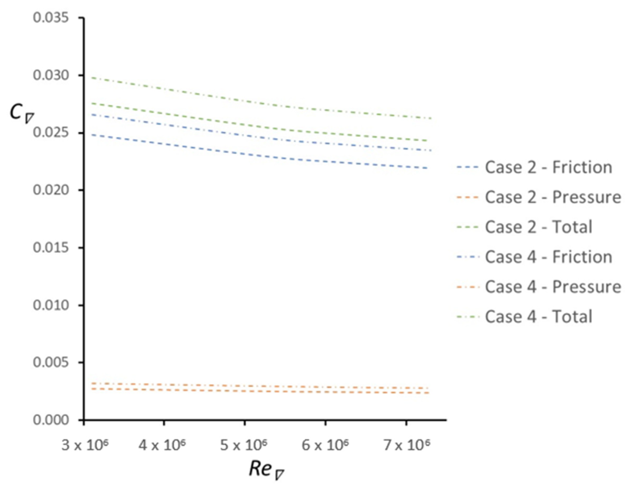
Figure 10 is a plot of the resistance coefficient, C∇, as a function of the Reynolds number, Re∇, for the U209 without a casing (Case 2) and with a casing (Case 4).
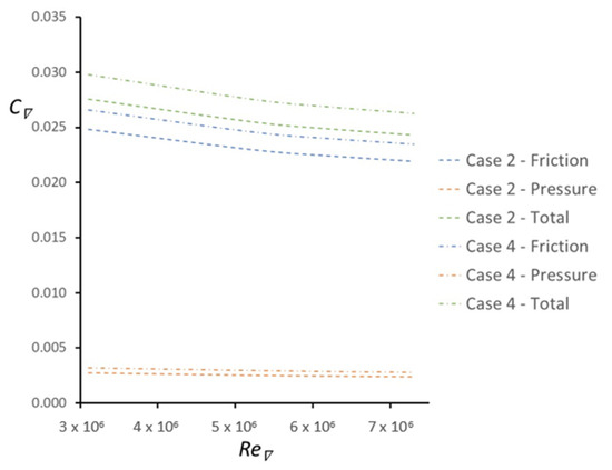
Figure 10.
Resistance coefficient as a function of Reynolds number for U209 without and with a casing (Case 2 = no casing; Case 4 = with casing).
The increase in wetted surface area as a result of the casing is about 8%, which results in an increase in friction resistance of approximately 7%. The increase in pressure resistance coefficient caused by the casing is about 18%, which compares with the value of 15% derived empirically and given in reference [9] for a simple casing.
The overall increase in resistance coefficient as a result of the casing is approximately 8%.
3.3. Influence of Sail
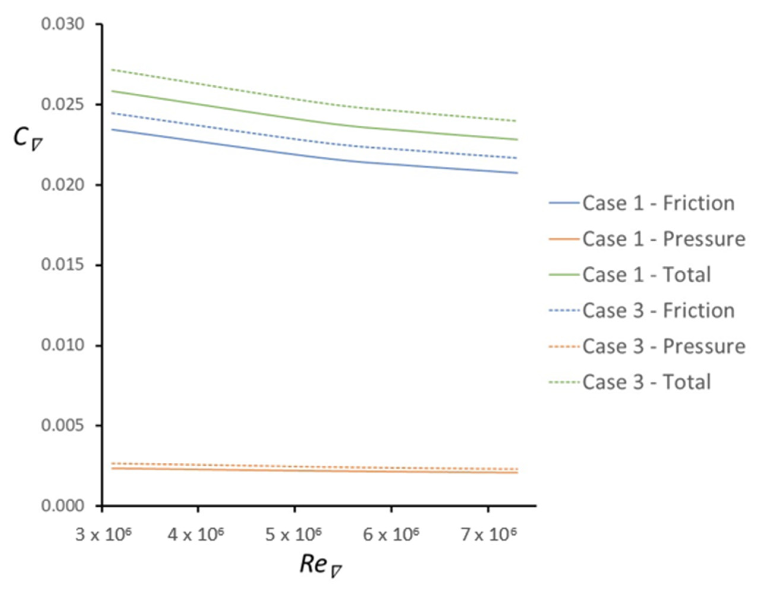
Figure 11 is a plot of resistance coefficient, C∇, as a function of the Reynolds number, Re∇, for the Suboff without sail (Case 1) and with a sail (Case 3). Note that, as can be seen from Figure 1, the Suboff sail is small compared to the size of the hull, which corresponds to that of a large nuclear-powered submarine.
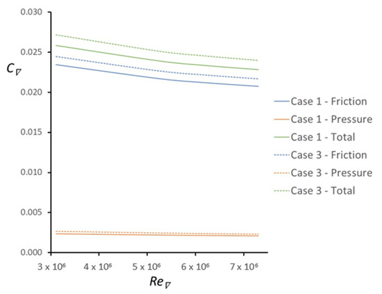
Figure 11.
Resistance coefficient as a function of Reynolds number for Suboff without and with a sail (Case 1 = no sail; Case 3 = with sail).
The increase in wetted surface area as a result of the addition of the small sail to the Suboff is about 2%, which results in an increase in friction resistance coefficient of approximately 4%. The increase in pressure resistance coefficient due to the sail is approximately 11% of the pressure resistance. Although this percentage increase seems large, it has to be remembered that the pressure resistance is only a very small component of the total resistance, and the pressure resistance of the Suboff is quite small.
The overall increase in resistance coefficient due to the sail on the Suboff being approximately 5%.
Figure 12 is a plot of resistance coefficient, C∇, as a function of the Reynolds number, Re∇, for the U209 without a sail (Case 4), with a small “Suboff” sail (Case 5), and with the larger U209 sail (Case 6). In each case, there is the same casing.
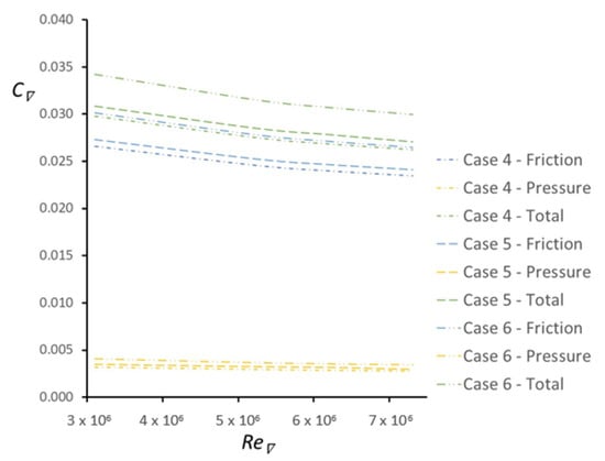
Figure 12.
Resistance coefficient as a function of Reynolds number for U209 without a sail, with a Suboff sail, and with a U209 sail (Case 4 = no sail; Case 5 = with Suboff sail; Case 6 with U209 sail).
The increase in wetted surface area by adding the Suboff sail to U209 with the casing is approximately 2%, and the increase in friction resistance coefficient is approximately 3%. The increase in pressure resistance coefficient when adding the Suboff sail to the U209 with casing is approximately 5%. The increase in total resistance coefficient when adding the Suboff sail to the U209 with casing is approximately 4%.
The increase in wetted surface area by adding the U209 sail to the U209 with only the casing is approximately 7.5%, and the corresponding increase in friction resistance coefficient is approximately 13%. The increase in pressure resistance coefficient when adding the U209 sail to the U209 hull with casing is approximately 23%. The resulting total increase in resistance coefficient for the U209 with the U209 sail, compared to the U209 with the casing alone, is approximately 14%.
3.4. Comparison with Empirical Prediction
The results for all six cases are compared with empirical predictions made using the method described in [9] in Table 3 and Figure 13 for a volumetric Reynolds number of 6.21 × 10⁶.
Table 3.
Resistance coefficient components (×10−3).
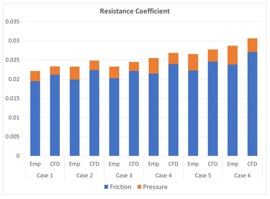
Figure 13.
Comparison between empirical prediction (Emp) and Computational Fluid Dynamics (CFD) for all cases.
As can be seen from Table 3 and Figure 9, the empirical resistance method described in [9] consistently underpredicts the total frictional resistance coefficient by about 10%. The equation for friction resistance used in [9] is given as Equation (6).
where:
The factor accounts for the friction form resistance of the axisymmetric hull form, and was added to account for the effect of L/D, based on CFD data for three axisymmetric hull forms obtained by Leong [35]. The value of used in [9] was 0.3 based on the results from Leong [35]. Further work is required to investigate whether modifications to Equations (6) and (7) are required to improve the empirical estimation of frictional resistance coefficient given in [9].
Note that Equation (6) gives the frictional resistance coefficient, , non-dimensionalized using the wetted surface, rather than the usable volume. Equation (8) is used to convert this to C∇, which is non-dimensionalized using the volume.
As noted above, the volume used in Equation (8) is the usable volume, which is the same for each of the submarine hull forms, and hence the results given in the paper are internally consistent and can be compared meaningfully.
Also, as can be seen from Table 3 and Figure 13, the empirical resistance method described in [9] significantly overpredicts the total pressure resistance coefficient by approximately 25–40%.
In [9], the pressure resistance coefficient is obtained from Equation (9).
is given by Equation (10).
where is the length of the parallel middle body, and the values of the constants can be obtained from Table 4.
Table 4.
Values of constants for Equation (10).
In Equation (10), the first term in the square brackets represents the pressure resistance on a hull with no parallel middle body and the second term accounts for parallel middle body. The values of the constants given in Table 4 have been obtained from data provided by [35].
Further work is required to investigate whether modifications are required to Equation (10) and/or the constants in Table 4 to improve the empirical estimate of pressure resistance coefficient presented in [9].
However, it is worth noting that the estimate of the total resistance coefficient obtained using the empirical method is consistently only about 5% lower than the values obtained from the present CFD method.
4. Concluding Remarks
The resistance coefficients for two different submarine geometries, scaled to have the same useable volume, were obtained using CFD. One of these is the well-known Suboff geometry, an axisymmetric hull with a parallel middle body, and the other the U209 hull form, designed with surface, as well as submerged, operations in mind.
The total resistance coefficient for the U209 bare hull is approximately 6% higher than that for the Suboff bare hull. This quantifies the advantage, in terms of submerged resistance, of a hull form specifically designed for underwater performance, compared to an older design where operation on the surface was also considered.
When a casing was added to the U209 geometry the increase in total resistance coefficient was approximately 8%. This quantifies clearly the disadvantage, in terms of submerged resistance, of fitting a casing to a submarine. Part of this increase is due to an increase in wetted surface area, and that can be obtained simply by allowing for the increased area. The increase due to pressure resistance is about 18%, which compares with the value of 15% derived empirically and given in [9]. Whilst there may be practical reasons for a casing on a submarine, the designer needs to be aware of the hydrodynamic disadvantage to doing this.
When the Suboff sail was added to the Suboff geometry, the overall increase in total resistance coefficient was approximately 5%.
When the Suboff sail was added to the U209 geometry, with a casing, the overall increase in resistance coefficient was approximately 4%, and when the U209 sail was added instead, the increase in resistance coefficient was approximately 14%. This is because the U209 sail is much larger than the Suboff sail.
Thus, the disadvantage, from a resistance point of view, of fitting a small or a large sail to the submarine hull can be quantified.
The empirical resistance prediction method given in [9] consistently underpredicts the friction resistance coefficient by approximately 10% and overpredicts the pressure resistance coefficient by approximately 25–40%. However, the empirical prediction of the total resistance coefficient is only about 5% too low. More work is required to improve the empirical resistance prediction method.
Author Contributions
Conceptualization, I.K.A.P.U. and M.R.; methodology, A.N. and S.; software, A.N.Y.; validation, I.K.A.P.U. and S.; formal analysis, A.N.; investigation, S.; resources, E.J.; data curation, E.J.; writing—original draft preparation, A.N. and S.; writing—review and editing, I.K.A.P.U. and M.R.; visualization, A.N.Y.; supervision, I.K.A.P.U. and M.R.; project administration, A.N.; funding acquisition, I.K.A.P.U. All authors have read and agreed to the published version of the manuscript.
Funding
This research was funded by Institut Teknologi Sepuluh Nopember under Inbound Researcher Mobility Program (IRM) 2024, based on Rector’s Decree Number: 137/IT2/T/HK.00.01/V/2024 dated 3 May 2024.
Institutional Review Board Statement
Not applicable.
Informed Consent Statement
Not applicable.
Data Availability Statement
All data are represented within the paper.
Acknowledgments
The authors are grateful to the Department of Naval Architecture, Faculty of Marine Technology, Institut Teknologi Sepuluh Nopember for the computing facility.
Conflicts of Interest
The authors declare no conflicts of interest.
References
- Clark, B. The Emerging Era in Undersea Warfare; The Center for Strategic and Budgetary Assessments (CSBA): Washington, DC, USA, 2015. [Google Scholar]
- Kiser, D.E. Indian, Japanese, and US Responses to Chinese Submarine Modernization. Ph.D. Thesis, Naval Postgraduate School, Monterey, CA, USA, 2016. [Google Scholar]
- The 2021 Military Balance Chart: Submarines and Sub-surface Warfare. Mil. Balance 2021, 121, ci. [CrossRef]
- Chapter One: Defence and military analysis. Mil. Balance 2021, 121, 9–22. [CrossRef]
- Benere, D.E. A Critical Examination of the US Navy’s Use of Unrestricted Submarine Warfare in the Pacific Theater During World War II; Naval War College, Joint Operations Department: Newport, RI, USA, 1992. [Google Scholar] [CrossRef]
- Humphris, S.E. Vehicles for deep sea exploration. In Elements of Physical Oceanography: A Derivative of the Encyclopedia of Ocean Sciences; Academic Press: Cambridge, MA, USA, 2009; pp. 197–209. [Google Scholar] [CrossRef]
- Groves, N.C.; Huang, T.T.; Chang, M.S. Geometric Characteristics of DARPA SUBOFF Models (DTRC Model Nos. 5470 and 5471); David Taylor Research Center: Bethesda, MD, USA, 1989. [Google Scholar]
- Liu, H.L.; Huang, T.T. Summary of DARPA SUBOFF Experimental Program Data; Report Number: CRDKNSWC/HD-1298-11; Naval Surface Warfare Center Carderock (NSWCCD): Bethesda, MD, USA, 1998. [Google Scholar] [CrossRef]
- Renilson, M.R. Submarine Hydrodynamics, 2nd ed.; Springer: Berlin/Heidelberg, Germany, 2018; ISBN 978-3-319-79056-5. [Google Scholar]
- Zheku, V.V.; Villa, D.; Piaggio, B.; Gaggero, S.; Viviani, M. Assessment of Numerical Captive Model Tests for Underwater Vehicles: The DARPA SUB-OFF Test Case. J. Mar. Sci. Eng. 2023, 11, 2325. [Google Scholar] [CrossRef]
- Uzun, D.; Sezen, S.; Atlar, M.; Turan, O. Effect of biofouling roughness on the full-scale powering performance of a submarine. Ocean Eng. 2021, 238, 109773. [Google Scholar] [CrossRef]
- Utama, I.K.A.P.; Farhan, F.; Nasirudin, A.; Ariesta, R.C.; Renilson, M.R. CFD Analysis of Biofouling Effect on Submarine Resistance and Wake. J. Mar. Sci. Eng. 2023, 11, 1312. [Google Scholar] [CrossRef]
- Lyu, X.; Tang, H.; Sun, J.; Wu, X.; Chen, X. Simulation of microbubble resistance reduction on a suboff model. Brodogradnja 2014, 65, 23–32. [Google Scholar]
- Kinaci, O.K.; Gokce, M.K.; Alkan, A.D.; Kukner, A. On self-propulsion assessment of marine vehicles. Brodogradnja 2018, 69, 29–51. [Google Scholar] [CrossRef]
- Chase, N.; Carrica, P.M. Submarine propeller computations and application to self-propulsion of DARPA Suboff. Ocean Eng. 2013, 60, 68–80. [Google Scholar] [CrossRef]
- Byeon, C.Y.; Kim, J.I.; Park, I.R.; Seol, H.S. Resistance and self-propulsion simulations for the DARPA Suboff submarine by using RANS method. J. Compt. Fluids Eng. 2018, 23, 36–46. [Google Scholar] [CrossRef]
- Delen, C.; Kinaci, O.K. Direct CFD simulations of standard maneuvering tests for DARPA Suboff. Ocean Eng. 2003, 276, 114202. [Google Scholar] [CrossRef]
- Nugroho, W.H.; Purnomo, N.J.H.; Suwarni, E.; Priohutomo, R.K.; Mulyad. Slamming loads prediction on a submarine hull structure. J. Subsea Offshore 2016, 8, 15–21. [Google Scholar]
- Utama, I.K.A.P.; Aryawan, W.D.; Nasirudin, A.; Sutiyo; Yanuar. Numerical Investigation into the Pressure and Flow Velocity Distributions of a Slender-Body Catamaran Due to Viscous Interference Effects. Int. J. Technol. 2021, 149-162, 149–162. [Google Scholar] [CrossRef]
- Mikulec, M.; Piehl, H. Verification and validation of CFD simulations with full-scale ship speed/power trial data. Brodogradnja 2023, 74, 41–62. [Google Scholar] [CrossRef]
- Hadi, E.S.; Tuswan, T.; Azizah, G.; Ali, B.; Samuel, S.; Hakim, M.L.; Hadi, M.R.C.P.; Iqbal, M.; Sari, D.P.; Satrio, D. Influence of the canal width and depth on the resistance of 750 DWT Perintis ship using CFD simulation. Brodogradnja 2023, 74, 117–144. [Google Scholar] [CrossRef]
- Trimulyono, A.; Hakim, M.L.; Ardhan, C.; Ahmad, S.T.P.; Tuswan, T.; Santosa, A.W.B. Analysis of the double steps position effect on planing hull performances. Brodogradnja 2023, 74, 41–72. [Google Scholar] [CrossRef]
- Dai, K.; Li, Y.; Gong, J.; Fu, Z.; Li, A.; Zhang, D. Numerical study on propulsive factors in regular head and oblique waves. Brodogradnja 2022, 73, 37–56. [Google Scholar] [CrossRef]
- Querard, A.B.G.; Temarel, P.; Turnock, S.R. Influence of viscous effects on the hydrodynamics of ship-like sections undergoing symmetric and antisymmetric motions, using RANS. In Proceedings of the ASME 27th International Conference on Offshore Mechanics and Arctic Engineering (OMAE), Estoril, Portugal, 5–20 June 2008; pp. 1–10. [Google Scholar] [CrossRef]
- Kim, S.P.; Lee, H.H. Fully nonlinear seakeeping analysis based on CFD simulations. In Proceedings of the 21st International Offshore and Polar Engineering Conference, Maui, HI, USA, 19–24 June 2011; pp. 970–974. [Google Scholar]
- Enger, S.; Peric, M.; Peric, R. Simulation of flow around KCS-hull. In Proceedings of the Gothenburg 2010—A Workshop on Numerical Ship Hydrodynamics, Gothenburg, Sweden, 8–10 December 2010. [Google Scholar]
- Tezdogan, T.; Demirel, Y.K.; Kellett, P.; Khorasanchi, M.; Incecik, A.; Turan, O. Full-scale unsteady RANS CFD simulations of ship behaviour and performance in head seas due to slow steaming. Ocean Eng. 2015, 97, 186–206. [Google Scholar] [CrossRef]
- Cakici, F.; Sukas, O.F.; Kinaci, O.K.; Alkan, A.D. Prediction of the vertical motions of dtmb 5415 ship using different numerical approaches. Brodogradnja 2017, 68, 29–44. [Google Scholar] [CrossRef]
- Park, J.; Seok, W. Computational analysis of strut effects on a BB2 submarine at drift angle 0, 6, and 12°. Int. J. Nav. Archit. Ocean Eng. 2023, 15, 100555. [Google Scholar] [CrossRef]
- Mai, T.L.; Jeon, M.; Vo, A.K.; Yoon, H.K.; Kim, S.; Lee, J. Establishment of empirical formula for hydrodynamic derivatives of submarine considering design parameters. Int. J. Nav. Archit. Ocean Eng. 2023, 15, 100537. [Google Scholar] [CrossRef]
- Roache, P.J. Perspective: A method for uniform reporting of grid refinement studies. ASME J. Fluids Eng. 1994, 116, 405–413. [Google Scholar] [CrossRef]
- Bayraktar, E.; Mierka, O.; Turek, S. Benchmark computations of 3D laminar flow around a cylinder with CFX, OpenFOAM and FeatFlow. Int. J. Comput. Sci. Eng. 2012, 7, 253–266. [Google Scholar] [CrossRef]
- Julián, I.; Herguido, J.; Menéndez, M. Gas permeation effect on the two-section two-zone fluidized bed membrane reactor (TS-TZFBMR) fluid dynamics: A CFD simulation study. Chem. Eng. J. 2016, 305, 201–211. [Google Scholar] [CrossRef]
- Utama, I.K.A.P.; Suastika, I.K.; Sulisetyono, A.; Hermawan, Y.A.; Aryawan, W.D. Resistance Analysis of Rescue Boat in Calm Water Condition. In IOP Conference Series: Materials Science and Engineering; IOP Publishing: Bristol, UK, 2021; Volume 1052, p. 012062. [Google Scholar] [CrossRef]
- Leong, Z.Q. (Australian Maritime College, University of Tasmania, Launceston, Tasmania, Australia). Personal Communication, 2017.


Disclaimer/Publisher’s Note: The statements, opinions and data contained in all publications are solely those of the individual author(s) and contributor(s) and not of MDPI and/or the editor(s). MDPI and/or the editor(s) disclaim responsibility for any injury to people or property resulting from any ideas, methods, instructions or products referred to in the content. |
© 2025 by the authors. Licensee MDPI, Basel, Switzerland. This article is an open access article distributed under the terms and conditions of the Creative Commons Attribution (CC BY) license (https://creativecommons.org/licenses/by/4.0/).