Data-Driven Koopman Based System Identification for Partially Observed Dynamical Systems with Input and Disturbance

Abstract

The identification of dynamical systems from data is essential in control theory, enabling the creation of mathematical models that accurately represent the behavior of complex systems. However, real-world applications often present challenges such as the unknown dimensionality of the system and limited access to measurements, particularly in partially observed systems. The Hankel alternative view of Koopman (HAVOK) method offers a data-driven approach to identify linear representations of nonlinear systems, but it often overlooks the influence of external control signals (inputs) and disturbances. This paper introduces a novel input-aware modeling method for unstable linear systems using data-driven Koopman analysis. By explicitly incorporating the impact of inputs and disturbances, our method enhances the accuracy and robustness of system identification, even in the face of incomplete observations. The proposed approach leverages Koopman operator theory on augmented state-input data to capture both the intrinsic dynamics and the system’s sensitivity to external control. Through extensive numerical examples, we demonstrate the effectiveness of our method in accurately identifying and predicting the behavior of various dynamical systems, including real-world nonlinear systems and simulated unstable linear systems with and without disturbances. The results highlight the potential of our approach to advance the field of system identification and control, offering a powerful tool for modeling and analyzing complex systems in diverse applications.

1. Introduction

In the field of scientific and engineering, it is essential to have an accurate mathematical model of dynamical systems, as it underpins control design, optimization, and performance analysis [1,2,3,4]. However, real-world systems are often intricate, demanding a deep understanding of their dynamics for optimal behavior. A major challenge arises in practical applications where only a subset of the system’s state variables are directly measurable. This limitation, known as the closure problem [5,6], renders direct inference of the complete state vector $\left(x\right)$ from the available measurements $\left(y\right)$ impossible.

The closure problem presents a significant hurdle for scientific modeling due to several factors. Limited access to observations can render closed-form models infeasible, making the construction of explicit models for hidden variables impractical [7]. This ultimately hinders the accurate simulation and prediction of the system’s behavior.

Conversely, statistical learning, machine learning, and system identification are interrelated fields that deal with extracting knowledge from data. At its core, this knowledge extraction process aims to transform raw data into actionable insights and predictive models. Statistical learning provides the foundation by analyzing data to reveal hidden patterns and relationships [8,9]. These patterns can range from simple correlations to complex, multi-dimensional structures. Machine learning builds on this, creating algorithms that automatically learn and improve on specific tasks from data, such as classification or prediction [10]. This learning process often involves adjusting internal parameters to minimize errors and optimize performance. System identification, a specialized field within machine learning, focuses on building mathematical models of dynamical systems from input-output data [11,12]. These models can be used to simulate, predict, and control the behavior of complex systems like robots, power grids, and even biological processes. In essence, statistical learning provides the groundwork for understanding data, machine learning allows algorithms to learn and improve on tasks, and system identification leverages this learning to create models of real-world systems.

However, traditional system identification techniques heavily rely on input-output (I/O) data, model structure (order and type), and selection criteria (rank and cost function) [13]. However, this approach presents a significant challenge to balancing model complexity with real-world applicability. While a high-order model can theoretically capture the exact dynamics of a system, regardless of its nature (linear/nonlinear, time-invariant/time-variant), it comes at a cost [14,15,16,17]. Increased model complexity can lead to difficulties in validation, as the model may fit noise alongside the actual system behavior. Additionally, designing control algorithms for such high-order models becomes cumbersome, hindering practical implementation.

On the other hand, Koopman operator theory offers a robust framework for identifying and controlling nonlinear dynamical systems by transforming them into a higher-dimensional linear space [18]. Through the utilization of singular value decomposition (SVD) for approximate the Koopman operator, recent advancements have focused on data-driven methods that leverage input-output data to construct Koopman-based models capable of handling disturbances and inputs effectively [19,20]. For instance, these methods have been applied to control robotic systems with high precision, despite the presence of nonlinearities and external disturbances [21]. Similarly, they have been used to design power system stabilizers that enhance the stability of power networks under various disturbance conditions [22,23,24].

Moreover, the Koopman operator framework has been extended to incorporate control inputs, leading to the development of bilinear models that offer enhanced control capabilities [25,26]. These models allow for the integration of modern control techniques, such as model predictive control (MPC), to manage complex dynamical systems efficiently [27,28]. While Koopman operator theory offers significant advantages, a key challenge lies in its infinite dimensionality. For practical applications, finite-dimensional approximations are necessary. Existing methods like Dynamic Mode Decomposition (DMD) [29,30], Extended DMD (EDMD) [31,32], and Tunable Accuracy Symmetric Subspace Decomposition (T-SSD) [33].

In this paper, the Koopman operator is applied within the Hankel Alternative View of Koopman (HAVOK) method for scenarios involving partially observed systems by proposing a novel-aware modeling method for unstable linear systems. The traditional HAVOK method offers a data-driven approach to identifying nonlinear systems through linear representations that focus on state dynamics, our proposed method comprises the influence of the input and offers robustness to external disturbances. The organization of this work as follows. In Section 2, we represent the problem formulation and the brief reviews of the Koopman operator. Moving on, Section 3 describes the proposed method for identifying an input influences dynamical system through a data-driven Koopman operator, Low rank approximation method also was presented to approximate a given matrix with lower rank based on linear algebra technique. In Section 4, we showcase numerical examples to demonstrate the effectiveness of the proposed method based on 3 cases of dynamical systems (real-world nonlinear system, simulated unstable linear system, and simulated an unstable linear system with input disturbance). Finally, we conclude the proposed approach to the system identification based on the data-driven Koopman Analysis with a novel input-aware modeling technique in Section 5.

2. Background

2.1. Problem Formulation

In system identification scheme, due to the fact that most of real-world dynamical systems are nonlinear, the main objective is to identify the nonlinear dynamical system

$$\dot{x}\left(t\right)=f\left(x\right(t),u(t\left)\right),$$

(1)

where $x\left(t\right)\in {\mathbb{R}}^n$ denotes the state variable, $u\left(t\right)\in {\mathbb{R}}^m$ represents the input, and $f(·,·)$ is a nonlinear function that describe the dynamics. According to Koopman Operator Theory [34], the system (1) can be linearized and approximate to linear state space model of the form

$$\left\{\begin{array}{c}\dot{x}\left(t\right)=Ax\left(t\right)+Bu\left(t\right)\hfill \\ y\left(t\right)=Cx\left(t\right)+Du\left(t\right)\hfill \end{array}\right.,$$

(2)

where $y\left(t\right)\in {\mathbb{R}}^l$ signifies the measured output. $A\in {\mathbb{R}}^{n\times n}$, $B\in {\mathbb{R}}^{n\times m}$, $C\in {\mathbb{R}}^{l\times n}$, and $D\in {\mathbb{R}}^{l\times n}$ are the matrices with appropriate size to be determined.

This poses a challenge in determining whether the available measurements are sufficient for accurately modeling the system. For instance, the dimension l of the measured output might be smaller than the actual state dimension n of the state space. In this work, we focus specifically on the scenario where $D=0$ and $l=1$, meaning the system has no feed-forward and we have access to only a one-dimensional time-series measurement for the system.

It’s important to note that the dimensionality of the underlying dynamics is often unknown in practice, and the choice of measurements may be limited by various constraints.

2.2. A Brief Review on Koopman Operator Theory

In 1931, B.O. Koopman established a foundational framework for the analysis of nonlinear dynamical systems, demonstrating that any autonomous nonlinear system can be represented as a linear system of infinite order within a Hilbert space [34].

Consider a continuous-time autonomous nonlinear dynamical system described by the following equation:

$$\dot{x}\left(t\right)=\mathcal{F}\left(x\right),$$

(3)

where $\mathcal{F}:{\mathbb{R}}^n\to {\mathbb{R}}^n$ defines the system dynamics. We are interested in a set of observables, denoted by $g\left(x\right):{\mathbb{R}}^n\to \mathbb{R}$, which are scalar-valued functions of the state that represent the system’s output. The Koopman operator, denoted by $\mathcal{K}\in \mathcal{B}\left(x\right)\to \mathcal{B}\left(x\right)$, where $\mathcal{B}\left(x\right)$ is the space of bounded measurable functions, acts on observable functions $g\in \mathcal{B}\left(x\right)$ according to

$$\mathcal{K}g\left(x\right)=g\circ \mathcal{F}\left(x\right).$$

(4)

where ∘ represents the composition operator, which essentially applies the function $\mathcal{F}$ to the state vector and then evaluates g on the resulting state. Then, a subspace $\mathcal{H}\subset \mathcal{B}\left(x\right)$ is said to be Koopman-invariant if

$$\begin{array}{c}\hfill \mathcal{K}\left(\mathcal{H}\right)\subseteq \mathcal{H}.\end{array}$$

(5)

In other words, a Koopman-invariant subspace is a collection of observable functions such that the Koopman operator, when applied to any function within the subspace, also produces a function within the same subspace. This property allows us to restrict the Koopman operator to the Koopman-invariant subspace, effectively reducing the problem to a finite-dimensional analysis within $\mathcal{H}$.

By analyzing the spectral properties of the Koopman operator, valuable insights into the system’s behavior can be obtained. These properties enable the expression of system dynamics as a linear system in a higher-dimensional space as

$$\dot{x}\left(t\right)=\mathcal{K}g\left(x\right)=Ax\left(t\right).$$

(6)

In this equation, A represents a linear operator derived from the Koopman operator and g. It governs the state propagation over time, despite the original system dynamics being nonlinear.

There are crucial to determine Koopman-invariant subspace and compute the matrix A in (6) as the choice of observable functions significantly impacts the resulting Koopman-invariant subspace and the accuracy of the finite-dimensional approximation. To address this challenge, various methods have been developed to identify Koopman-invariant subspaces and compute the matrix A in (6). One widely used method is Dynamic Mode Decomposition (DMD) [29,30,31,32]. DMD leverages a technique called Singular Value Decomposition (SVD) to factorize a data-driven approximation of the system’s state transition matrix. This factorization reveals the system’s dynamic modes, ordered by their decreasing magnitude.

3. Proposed Method

This section details the proposed methodology for identifying how an input influences a dynamical system through a data-driven Koopman operator. Additionally, we include the technique used for low-rank approximation.

3.1. Data-Driven Koopman Operator

Consider a Least Square Estimation (LSE) problem of the form:

$$\dot{y}=\mathrm{\Theta }\left(Y\right){\mathrm{\Xi }}^T,$$

(7)

where $\dot{y}$ is a time-derivative of vector y, the library matrix $\mathrm{\Theta }\left(Y\right)$ is

$$\mathrm{\Theta }\left(Y\right)=\left[\begin{array}{ccccc}|& |& |& \dots & |\\ y_1& y_2& y_3& \dots & y_r\\ |& |& |& \dots & |\end{array}\right],$$

(8)

where $\mathrm{\Xi }\in {\mathbb{R}}^{(r+1)\times r}$. Each row ${\xi }_k$ in $\mathrm{\Xi }$ is a vector of coefficients determining the active terms in the k-th column in the library matrix (8). Then we construct the Hankel matrix of measured data $y\left(t\right)$ as

$$H=\left[\begin{array}{cccc}y\left(t_1\right)& y\left(t_2\right)& \dots & y\left(t_p\right)\\ y\left(t_2\right)& y\left(t_3\right)& \dots & y\left(t_{p+1}\right)\\ \\ ⋮& ⋮& \ddots & ⋮\\ y\left(t_q\right)& y\left(t_{q+1}\right)& \dots & y\left(t_m\right)\end{array}\right].$$

(9)

This Hankel matrix can be related to the Koopman operator:

$$\begin{array}{c}\hfill H=\left[\begin{array}{cccc}\mathcal{K}y\left(t_1\right)& {\mathcal{K}}^{2}y\left(t_1\right)& \dots & {\mathcal{K}}^{p}y\left(t_1\right)\\ {\mathcal{K}}^{2}y\left(t_1\right)& {\mathcal{K}}^{3}y\left(t_1\right)& \dots & {\mathcal{K}}^{p+1}y\left(t_1\right)\\ \\ ⋮& ⋮& \ddots & ⋮\\ {\mathcal{K}}^{q}y\left(t_1\right)& {\mathcal{K}}^{q+1}y\left(t_1\right)& \dots & {\mathcal{K}}^{m}y\left(t_1\right)\end{array}\right],\end{array}$$

(10)

by the used of SVD, as it will be described later, the low rank approximation of H is defined as

$$\hat{H}\approx U_r{\Sigma }_r{V}_r^T,$$

(11)

where $\widehat{H}$ is rank r approximation of H.

Mirroring the structure of the initial LSE problem, we formulate another LSE problem using the matrix $V_r$ which represents the system dynamics:

$${\dot{V}}_r=\mathrm{\Theta }\left(V_r\right){\mathrm{\Xi }}^T.$$

(12)

where ${\dot{V}}_r={\left[\begin{array}{cccc}{\dot{v}}_1& {\dot{v}}_2& \dots & {\dot{v}}_r\end{array}\right]}^T$, $\mathrm{\Xi }\in {\mathbb{R}}^{r\times r+1}$ each column ${\xi }_k$ in $\mathrm{\Xi }$ is a vector of coefficients determining the active terms in the kth column in $\mathrm{\Theta }\left(V_r\right)$.

Given that the measurement data $y\left(t\right)$ is sampled with a period $\mathrm{\Delta }t$, we approximate the second-order central derivative of the unitary matrix $V_r\left(t\right)$ with approximation error of $O\left(\mathrm{\Delta }{t}^2\right)$

$$\begin{array}{c}\hfill {\dot{V}}_r={\displaystyle \frac{{\displaystyle d{V}_r\left(t\right)}}{{\displaystyle dt}}}\approx {\displaystyle \frac{{\displaystyle V_r(t+1)-V_r(t-1)}}{{\displaystyle 2\mathrm{\Delta }t}}}+O\left(\mathrm{\Delta }{t}^2\right).\end{array}$$

(13)

To incorporate the input, the input vector $u\left(t\right)$ has been append to the last column of the library matrix $\mathrm{\Theta }\left(V_r\right)$ as

$$\mathrm{\Theta }\left(V_r\right)=\left[\begin{array}{ccccc}|& |& \dots & |& |\\ v_1& v_2& \dots & v_r& u\left(t\right)\\ |& |& \dots & |& |\end{array}\right].$$

(14)

We can reinterpret the LSE problem as:

$$\dot{V_r}=\mathrm{\Theta }\left(V_r\right){\xi }_1+\mathrm{\Theta }\left(V_r\right){\xi }_2+\dots +\mathrm{\Theta }\left(V_r\right){\xi }_{r+1}.$$

(15)

Consequently, we find the values in $\mathrm{\Xi }$ by solving a convex $l_1$ regularized Least Absolute Deviations (LAD) regression where $ϵ$ is an arbitrary small positive number:

$$\begin{array}{cc}\hfill \mathrm{minimize}& \parallel {\xi }_k{\parallel }_1\hfill \\ \hfill \mathrm{subject}\mathrm{to}& \parallel {\dot{v}}_k-\mathrm{\Theta }\left(V\right){\xi }_k{\parallel }_1\le ϵ.\hfill \end{array}$$

(16)

The main algorithm (Algorithm 1) performs minimization of the $L1$ norm with an $L1$ constraint to find an optimal matrix $\mathrm{\Xi }$ that best represents the relationship between the matrices $\dot{V}$ and $\mathrm{\Theta }.$ It begins by initializing $\mathrm{\Xi }$ and iteratively updating it until convergence is achieved. In each iteration, a subproblem (Algorithm 2) is solved to refine $\mathrm{\Xi }$. The subproblem calculates the residual $R=\dot{V}-\mathrm{\Theta }\mathrm{\Xi }$ and finds a feasible direction D that aligns with the sign of R, adjusting $\mathrm{\Xi }$ in a way that minimizes the $L1$ norm. A line search is conducted to determine the optimal step size $\alpha$ that minimizes ${\parallel \mathrm{\Xi }+\alpha D\parallel }_1$ while maintaining the constraint $\parallel \mathrm{\Theta }\left(\mathrm{\Xi }+\alpha D\right)-\dot{V}{\parallel }_1\le ϵ$. This approach ensures that $\mathrm{\Xi }$ is iteratively refined under the $L1$ constraint, balancing sparsity and accuracy. The iterative process terminates once $\mathrm{\Xi }$ stabilizes, achieving a solution that minimizes the $L1$ norm within the given tolerance.

We opt for LAD over LSE due to its robustness against outliers, particularly in the presence of gross errors or heavy-tailed noise. This strengthens the proposed method’s resilience to noise and measurement inaccuracies. $\widehat{A}$ and $\widehat{B}$ are given using matrix of coefficients $\mathrm{\Xi }$ as

$$\begin{array}{ccc}\hfill \mathrm{\Xi }& =& \left[\begin{array}{ccccc}{\xi }_{1,1}& {\xi }_{1,2}& \dots & {\xi }_{1,r}& {\xi }_{1,r+1}\\ {\xi }_{2,1}& {\xi }_{2,2}& \dots & {\xi }_{2,r}& {\xi }_{2,r+1}\\ ⋮& ⋮& \ddots & ⋮& ⋮\\ {\xi }_{r,1}& {\xi }_{r,2}& \dots & {\xi }_{r,r}& {\xi }_{r,r+1}\end{array}\right]\hfill \\ & =& \left[\begin{array}{cc}\widehat{A}& \widehat{B}\end{array}\right],\hfill \end{array}$$

(17)

where

$$\begin{array}{c}\hfill \widehat{A}=\left[\begin{array}{cccc}{\xi }_{1,1}& {\xi }_{1,2}& \dots & {\xi }_{1,r}\\ {\xi }_{2,1}& {\xi }_{2,2}& \dots & {\xi }_{2,r}\\ ⋮& ⋮& \ddots & ⋮\\ {\xi }_{r,1}& {\xi }_{r,2}& \dots & {\xi }_{r,r}\end{array}\right]\end{array}$$

(18)

and

$$\begin{array}{c}\hfill \widehat{B}=\left[\begin{array}{c}{\xi }_{1,r+1}\\ {\xi }_{2,r+1}\\ ⋮\\ {\xi }_{r,r+1}\end{array}\right].\end{array}$$

(19)

For the matrix $\widehat{C}$ is determined as the first row of $U_r{\Sigma }_r$.

Algorithm 1 Minimization of L1 Norm with L1 Constraint

Input:  Matrices $\dot{V}\in {\mathbb{R}}^{m\times n}$, $\mathrm{\Theta }\in {\mathbb{R}}^{m\times p}$, tolerance $ϵ$ Output:  Matrix $\mathrm{\Xi }\in {\mathbb{R}}^{p\times n}$ 1: Initialize $\mathrm{\Xi }$ 2: repeat 3:     ${\mathrm{\Xi }}_{\mathrm{prev}}=\mathrm{\Xi }$ {Store previous iterate} 4:     Solve subproblem to update $\mathrm{\Xi }$ 5: until Convergence

Algorithm 2 Subproblem for Updating $\mathrm{\Xi }$

Input:  $\dot{V}$, $\mathrm{\Theta }$, $ϵ$, current $\mathrm{\Xi }$ Output:  Updated $\mathrm{\Xi }$ 1: $R=\dot{V}-\mathrm{\Theta }\mathrm{\Xi }$ {Residual} 2: Find a feasible direction D such that 3: $\mathrm{sign}\left(D_{ij}\right)=-\mathrm{sign}\left(R_{ij}\right)$ if $|R_{ij}|>0$ 4: and ${\parallel D\parallel }_1\le 1$ 5: Perform line search to find step size $\alpha$: 6: ${\alpha }^{*}=arg{min}_{\alpha \ge 0}{\parallel \mathrm{\Xi }+\alpha D\parallel }_1$ 7: subject to $\parallel \mathrm{\Theta }(\mathrm{\Xi }+\alpha D)-\dot{V}{\parallel }_1\le ϵ$ 8: Update $\mathrm{\Xi }$: $\mathrm{\Xi }\leftarrow \mathrm{\Xi }+{\alpha }^{*}D$

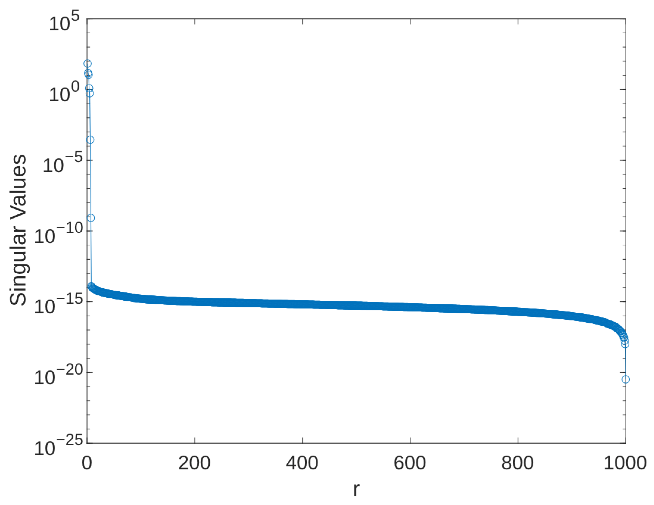
3.2. Low Rank Approximation Method

Low-rank approximation is a fundamental technique in linear algebra, where a given matrix is represented by another matrix of reduced rank. This process serves multiple purposes including dimensionality reduction, data compression, and the extraction of salient patterns from the original data. Given a matrix H, the objective is to identify a matrix $\widehat{H}$ of lower rank that optimally approximates H. The quality of this approximation is typically assessed using a matrix norm.

Figure 1 illustrates the magnitude of singular values across different ranks r, while Figure 2 offers a closer look at the magnitudes from $r=1$ to $r=20$. It is evident that only a few initial terms are required to capture the essential dynamics of the system. Consequently, the rank r can be determined visually.

In cases involving large matrices, the Partial SVD using Matrix Sketching [35] provides an efficient alternative. This approach constructs a “sketch” that encapsulates the key features of the matrix, thereby enabling the approximation of its singular value decomposition (SVD). A notable advantage of this method is its adaptive rank determination based on a predefined tolerance, eliminating the need to specify the rank a priori. This results in faster computation, making it particularly suitable when a full SVD is computationally expensive or when the appropriate rank is unknown. The accuracy of the approximation is adjustable through the tolerance parameter, allowing for a balance between computational efficiency and the desired level of precision. The detailed implementation steps are outlined in Algorithm 3.

Algorithm 3 Partial SVD using Matrix Sketching

Input:  Matrix $H\in {\mathbb{R}}^{m\times n}$, tolerance tol Output:  $U_r$, $S_r$, $V_r$ (approximate SVD of H) 1: Initialize $U=[]$, $V=[]$, $S=[]$ 2: $k=0$ {Rank of the sketch} 3: while approximation error > tol do 4:     $k=k+1$ 5:     Randomly sample a column c from H 6:     Orthogonalize c against the columns of U to get $u_k$ 7:     $U=[U,u_k]$ {Add $u_k$ to the basis} 8:     Randomly sample a row r from H 9:     Orthogonalize r against the rows of V to get $v_k$ 10:     $V=[V;v_k]$ {Add $v_k$ to the basis} 11: end while 12: $B=U^{T}AV$ {Project H onto the sketch space} 13: $[U_B,S_B,V_B]=\mathrm{svd}\left(B\right)$ {Compute SVD of the smaller matrix} 14: $U_r=U{U}_B$ 15: $S_r=S_B$ 16: $V_r=V{V}_B$

4. Numerical Examples

To evaluate the efficacy of the proposed method, we selected three distinct dynamical systems for investigation: a real-world nonlinear system, a simulated unstable linear system, and a simulated unstable linear system subjected to input disturbances. All experiments were conducted using MATLAB R2024a on a MacBook Pro (14-inch, 2021) equipped with an Apple M1 Pro 8-core CPU and 16 GB of unified memory. This hardware configuration was chosen to assess the method’s performance on a readily available computing platform, ensuring its accessibility and applicability to a wide range of researchers and practitioners.

4.1. Nonlinear System

For the nonlinear system evaluation, we utilized the dataset and reference models of the Electro-Mechanical Positioning System (EMPS) [36]. This dataset provides a comprehensive representation of a standard drive system configuration commonly found in prismatic joints of robots and machine tools. The data were acquired using a dSPACE digital control system with a sampling frequency of 1 kHz and a duration of approximately 25 s, capturing the rich dynamics of the EMPS under various operating conditions.

To assess performance, following a typical machine learning training process, the measured data have been spitted into train and test sets. The initial 10 s of data were employed as the training set. The rest of dataset were used as test set. This means 40% of data was used as train set and 60% is used as test set. The Hankel matrix H was constructed with $q=p=5000$. Our simulation results, as depicted in Figure 3, demonstrate the capability of the proposed method to forecast at least 20 s of system behavior using only 10 s of training data. Furthermore, the prediction error, visualized in Figure 4, remains relatively small, further attesting to the accuracy and effectiveness of the method in this nonlinear system scenario.

4.2. Unstable Linear System

Furthermore, the application of Koopman operator theory proves to be particularly advantageous in the identification process of unstable linear systems, offering a unique perspective and analytical tools to understand their complex dynamics. To illustrate this, let’s examine a representative unstable linear system characterized by the following matrices:

$$A=\left[\begin{array}{ccccc}0.99& 0.01& 0.18& -0.09& 0\\ 0& 0.94& 0& 0.29& 0\\ 0& 0.14& 0.81& -0.9& 0\\ 0& -0.2& 0& 0.95& 0\\ 0& 0.09& 0& 0& 0.9\end{array}\right],$$

$$B=\left[\begin{array}{c}0.01\\ -0.14\\ 0.05\\ 0.02\\ -0.01\end{array}\right],C=\left[\begin{array}{ccccc}0& 1& 0& 0& -1\\ 0& 0& 1& 0& 0\\ 0& 0& 0& 1& 0\\ 1& 0& 0& 0& 0\end{array}\right].$$

In this system, the vector $x\left(t\right)={\left[\begin{array}{ccccc}{x}_1\left(t\right)& x_2\left(t\right)& x_3\left(t\right)& x_4\left(t\right)& x_5\left(t\right)\end{array}\right]}^T$ represented the state variables, while the outputs are captured by $y\left(t\right)={\left[\begin{array}{cccc}{y}_1\left(t\right)& y_2\left(t\right)& y_3\left(t\right)& y_4\left(t\right)\end{array}\right]}^T$. The system is driven by an input signal defined as $u\left(t\right)=sin\left(\omega t\right)$.

For the purpose of this analysis, we make the assumption that only the first output, $y_1$, is available for measurement. This constraint reflects a realistic scenario where complete state observation might be impractical or impossible, further highlighting the utility of the Koopman-based approach in extracting meaningful system information from limited measurements.

To evaluate the effectiveness and accuracy of the proposed method, we conducted simulations of the system with parameters $\omega =1$ and $\mathrm{\Delta }t=0.001$. Time series data $y\left(t\right)$ was collected from the simulation, spanning from $t=0$ to $t=5$, resulting in 5000 samples for the measurement data vector, given the chosen simulation time step. The initial 2 s of data were employed as the training set. The rest of dataset were used as test set. This means 40% of data was used as train set and 60% is used as test set. The Hankel matrix H was then constructed with $q=p=1000$.

The outcomes of these time series prediction efforts are showcased in Figure 5, while Figure 6 provides a visualization of the corresponding prediction error. These figures offer insights into the method’s performance, particularly its ability to accurately predict the behavior of the unstable linear system under investigation.

The identified coefficient matrices are

$$\widehat{A}=\left[\begin{array}{ccccc}0.6626& 0.2648& 0.1426& -0.0217& 0\\ -0.0328& 0.4353& 0.0342& -0.0042& 0\\ 0.2844& -6.4921& -0.0743& -0.0099& 0\\ 5.8002& -7.5986& 0.1658& 1.1511& -0.0001\\ 2.5930& -0.4246& 0& 17.5583& 0.9088\end{array}\right],$$

$$\widehat{B}=\left[\begin{array}{c}0.0040\\ -0.2799\\ -0.0047\\ -0.0242\\ -0.0362\end{array}\right],$$

and

$$\widehat{C}=\left[\begin{array}{ccccc}1.0022& 0.4550& 0.0001& 0.0133& 0\end{array}\right].$$

4.3. Unstable Linear System with Input Disturbance

In addition to investigating the unstable linear system in Section 4.2, we also explored the influence of disturbances on the identification process. We introduced a disturbance generator into the linear system, described by

$$\begin{array}{ccc}\hfill {\dot{x}}_d\left(t\right)& =& A_d{x}_d\left(t\right)\hfill \\ \hfill y_d\left(t\right)& =& C_d{x}_d\left(t\right)\hfill \end{array}.$$

(20)

This disturbance generator was then incorporated into the original plant model, leading to an augmented system;

$$\begin{array}{ccc}\hfill {\dot{x}}_0\left(t\right)& =& A_0{x}_0\left(t\right)+B_{0}u\left(t\right)\hfill \\ \hfill y_0\left(t\right)& =& C_0{x}_0\left(t\right)\hfill \end{array},$$

(21)

where $x_0=\left[\begin{array}{c}x\\ x_d\end{array}\right]$, $A_0=\left[\begin{array}{cc}A& B{C}_d\\ 0& A_d\end{array}\right]$, $B_0=\left[\begin{array}{c}B\\ 0\end{array}\right]$, and $C_0=\left[\begin{array}{cc}C& 0\end{array}\right]$.

For our numerical example, we retained the same parameter matrices A, B, and C from the previous unstable linear system case, and introduced the following matrices for the disturbance generator:

$$A_d=\left[\begin{array}{cc}0& 1\\ -10& 0\end{array}\right],C_d=\left[\begin{array}{cc}1& 0\end{array}\right].$$

Similar to the previous example, the Hankel matrix H was constructed with parameters $q=p=1000$. Applying the proposed method to this augmented system yielded the following identified matrices:

$$\widehat{A}=\left[\begin{array}{ccccccc}-0.0764& 0.8656& -0.0002& 0.1047& -0.0366& -0.1479& 0.0000\\ -1.1933& 1.8177& -0.1190& 0.3936& -0.0763& -0.2691& 0.0001\\ 0.2463& 0.0093& -0.1991& -3.1713& 0.2899& 0.0625& 0.0001\\ -0.5049& 1.5165& 3.1884& 0.3364& -0.0775& -0.7332& 0.0002\\ -0.2920& 0.6841& 1.1492& 0.0762& 0.3508& -0.4892& 0.0001\\ -0.0532& -0.8513& 0.1012& -1.4484& 6.1917& -0.0324& 0.0000\\ -0.6698& -5.8829& 1.5594& -5.4843& 1.8886& -0.0000& 0.9133\end{array}\right],$$

$$\widehat{B}=\left[\begin{array}{c}-0.0043\\ -0.0112\\ 0.0002\\ -0.0464\\ 0.1669\\ -0.0020\\ -0.0115\end{array}\right],$$

$$\widehat{C}=\left[\begin{array}{ccccccc}-3.7384& 2.1729& 1.0037& 1.3466& -0.3981& -0.1606& -0.0002\end{array}\right].$$

Finally, to recover the original system matrices $A_0$, $B_0$, and $C_0$, a similarity transformation can be applied, utilizing the relationship $A_0=T\widehat{A}{T}^{-1}$, $B_0=T\widehat{B}$ and $C_0=\widehat{C}{T}^{-1}$

The outcomes of these time series prediction efforts, even in the presence of disturbances, are illustrated in Figure 7. Correspondingly, Figure 8 visualizes the prediction error associated with these forecasts. These figures offer valuable insights into the robustness and performance of the proposed method, particularly highlighting its capacity to accurately predict the behavior of the unstable linear system even when subjected to external disturbances.

4.4. Comparison to Existing System Identification Methods

This subsection presents a detailed evaluation of the proposed system identification method, comparing its performance against established techniques within the field. A single pendulum system is employed as a benchmark, ensuring a consistent and transparent assessment of each method’s capabilities. The comparative methods include the widely used N4SID algorithm [37], known for its robust performance across various applications; the Derivative-Based Koopman Operators [19], a newer approach with promising advantages in nonlinear system identification; and the proposed method, which seeks to address specific limitations of current techniques. This comparative analysis aims to highlight the strengths and weaknesses of each approach, providing insights into the proposed method’s effectiveness relative to established alternatives.

To generate the training dataset and train the Derivative-Based Koopman Operators model, we utilize Python code from [19], simulating 500 uniformly sampled initial states for 0.04 s with time steps of $\mathrm{\Delta }t=0.001$ s. The N4SID model is trained using MATLAB’s system identification toolbox. The test dataset was generated for 0.3 s with time steps of $\mathrm{\Delta }t=0.001$ s. Thus, 13% of data was used as train set and 87% is used as test set.

Figure 9 illustrates the time-series prediction performance across various techniques, where the proposed method and N4SID exhibit better performance in long-term predictions. In Addition,

Table 1. Comparison of some existing system identification methods for the single pendulum system.

Method	Basis Generation	Train NRMSE	Test NRMSE
N4SID	LQ decompostion and SVD	0.0486	0.0096
[19]	High-order derivative	0.0028	8.3228
Proposed	SVD	0.0010	0.0011

presents a detailed comparison of training and testing normalized root mean square error (NRMSE) across the selected system identification methods, highlighting the performance differences in handling the single pendulum system. The N4SID method, utilizing LQ decomposition and singular value decomposition (SVD), achieves a training NRMSE of 0.0486 and a notably lower testing NRMSE of 0.0096, demonstrating reliable predictive performance in linear scenarios but showing some limitations in the training phase. In contrast, the Derivative-Based Koopman Operators, which apply high-order derivatives, excel with a very low training NRMSE of 0.0028, suggesting effective internal learning of system dynamics. However, it exhibits a high testing NRMSE of 8.3228, indicating reduced capability for long term prediction. The proposed method, which also leverages SVD, yields the lowest NRMSE values in both training (0.0010) and testing (0.0011), underscoring its robustness and ability to generalize across varying conditions.

5. Conclusions

This paper introduced a data-driven methodology for the identification of the Koopman operator in dynamical systems, with a particular emphasis on accurately capturing the influence of inputs on the system’s dynamic behavior. The proposed approach effectively leverages the power of low-rank approximations and the inherent robustness of Least Absolute Deviations regression to extract meaningful representations from potentially noisy and incomplete measurements. The efficacy of this method has been rigorously validated through its application to a diverse range of dynamical systems, encompassing both real-world nonlinear systems and simulated linear systems, with and without the presence of external disturbances. The results unequivocally demonstrate the method’s proficiency in both system identification and time-series prediction tasks.

The proposed method’s strong performance in terms of accuracy and generalization suggests that it could be valuable for applications requiring precise system identification in nonlinear environments, such as robotics, control systems, and predictive maintenance. However, as the proposed method is open-loop identification method, the ability in closed-loop identification are still not covered in this study as the input may cannot measured. Despite those limitation, the method’s stability in prediction could lead to improved reliability and performance in these applications, supporting decision-making and system optimization.

References

1. Xu, L.; Li, X.R.; Liang, Y.; Duan, Z. Modeling and State Estimation of Linear Destination-Constrained Dynamic Systems. IEEE Trans. Signal Process. 2022, 70, 2374–2387. [Google Scholar] [CrossRef]
2. Wang, K.; Liu, M.; He, W.; Zuo, C.; Wang, F. Koopman Kalman Particle Filter for Dynamic State Estimation of Distribution System. IEEE Access 2022, 10, 111688–111703. [Google Scholar] [CrossRef]
3. Kang, T.; Peng, H.; Xu, W.; Sun, Y.; Peng, X. Deep Learning-Based State-Dependent ARX Modeling and Predictive Control of Nonlinear Systems. IEEE Access 2023, 11, 32579–32594. [Google Scholar] [CrossRef]
4. Makki, O.T.; Moosapour, S.S.; Mobayen, S.; Nobari, J.H. Design, Mathematical Modeling, and Control of an Underactuated 3-DOF Experimental Helicopter. IEEE Access 2024, 12, 55568–55586. [Google Scholar] [CrossRef]
5. Gupta, A.; Lermusiaux, P.F.J. Neural closure models for dynamical systems. R. Soc. Math. Phys. Eng. Sci. 2021, 477, 20201004. [Google Scholar] [CrossRef]
6. Freeman, D.C.; Giannakis, D.; Slawinska, J. Quantum Mechanics for Closure of Dynamical Systems. Multiscale Model. Simul. 2024, 22, 283–333. [Google Scholar] [CrossRef]
7. Agrawal, A.; Koutsourelakis, P.-S. A probabilistic, data-driven closure model for RANS simulations with aleatoric, model uncertainty. J. Comput. Phys. 2024, 508, 112982. [Google Scholar] [CrossRef]
8. Hastie, T.; Tibshirani, R.; Friedman, J. Textbook of The Elements of Statistical Learning Data Mining, Inference, and Prediction, 2nd ed.; Springer: New York, NY, USA, 2009; pp. 1–2. [Google Scholar]
9. James, G.; Witten, D.; Hastie, T.; Tibshirani, R.; Taylor, J. Textbook of An Introduction to Statistical Learning with Application in Python; Springer: New York, NY, USA, 2023; pp. 1–17. [Google Scholar]
10. Rainio, O.; Teuho, J.; Klén, R. Evaluation metrics and statistical tests for machine learning. Sci. Rep. 2024, 14, 6086. [Google Scholar] [CrossRef]
11. Wang, L.Y.; Yin, G.G.; Zhao, Y.; Zhang, J.-F. Identification Input Design for Consistent Parameter Estimation of Linear Systems With Binary-Valued Output Observations. IEEE Trans. Autom. Control 2008, 53, 867–880. [Google Scholar] [CrossRef]
12. Wigren, A.; Wagberg, J.; Lindsten, F.; Wills, A.G.; Schon, T.B. Nonlinear System Identification: Learning While Respecting Physical Models Using a Sequential Monte Carlo Method. IEEE Control Syst. Mag. 2022, 42, 75–102. [Google Scholar] [CrossRef]
13. Kwad, A.M.; Hanafi, D.; Omar, R.; Rahman, H.A. Development of system identification from traditional concepts to real-time soft computing based. In IOP Conference Series: Materials Science and Engineering; IOP Publishing: Bristol, UK, 2020; Volume 767. [Google Scholar]
14. Hjalmarsson, H. System Identification of Complex and Structured Systems. Eur. J. Control 2009, 15, 275–310. [Google Scholar] [CrossRef]
15. Rojas, C.R.; Barenthin, M.; Welsh, J.S.; Hjalmarsson, H. The cost of complexity in system identification: The Output Error case. Automatica 2011, 47, 1938–1948. [Google Scholar] [CrossRef]
16. Schoukens, J.; Marconato, A.; Pintelon, R.; Rolain, Y.; Schoukens, M.; Tiels, K.; Vanbeylen, L.; Vandersteen, G.; Mulders, A.V. System identification in a real world. In Proceedings of the 2014 IEEE 13th International Workshop on Advanced Motion Control (AMC), Yokohama, Japan, 14–16 March 2014; pp. 1–9. [Google Scholar]
17. Kabzinski, T.; Jax, P. A Flexible Framework for Expectation Maximization-Based MIMO System Identification for Time-Variant Linear Acoustic Systems. IEEE Open J. Signal Process. 2024, 5, 112–121. [Google Scholar] [CrossRef]
18. Brunton, S.L.; Brunton, B.W.; Proctor, J.L.; Kutz, J.N. Koopman Invariant Subspaces and Finite Linear Representations of Nonlinear Dynamical Systems for Control. PLoS ONE 2016, 11, 11–19. [Google Scholar] [CrossRef]
19. Mamakoukas, G.; Castaño, M.L.; Tan, X.; Murphey, T.D. Derivative-Based Koopman Operators for Real-Time Control of Robotic Systems. IEEE Trans. Robot. 2021, 37, 2173–2192. [Google Scholar] [CrossRef]
20. Xu, Y.; Wang, Q.; Mili, L.; Zheng, Z.; Gu, W.; Lu, S.; Wu, Z. A Data-Driven Koopman Approach for Power System Nonlinear Dynamic Observability Analysis. IEEE Trans. Power Syst. 2024, 39, 4090–4104. [Google Scholar] [CrossRef]
21. Jia, J.; Zhang, W.; Guo, K.; Wang, J.; Yu, X.; Shi, Y.; Guo, L. EVOLVER: Online Learning and Prediction of Disturbances for Robot Control. IEEE Trans. Robot. 2024, 40, 382–402. [Google Scholar] [CrossRef]
22. Choi, H.; Elliott, R.; Byrne, R. Data-Driven Power Flow Estimation with Inverter Interfaced Energy Storage Using Dynamic Injection Shift Factor. In Proceedings of the IEEE Power and Energy Society General Meeting (PESGM), Denver, CO, USA, 17–21 July 2022; pp. 1–5. [Google Scholar]
23. Zheng, L.; Liu, X.; Xu, Y.; Hu, W.; Liu, C. Data-driven Estimation for a Region of Attraction for Transient Stability Using the Koopman Operator. CSEE J. Power Energy Syst. 2023, 9, 1405–1413. [Google Scholar]
24. Sarić, A.A.; Transtrum, M.K.; Sarić, A.T.; Stanković, A.M. Integration of Physics- and Data-Driven Power System Models in Transient Analysis After Major Disturbances. IEEE Syst. J. 2023, 17, 479–490. [Google Scholar] [CrossRef]
25. Bruder, D.; Fu, X.; Vasudevan, R. Advantages of bilinear koopman realizations for the modeling and control of systems with unknown dynamics. IEEE Robot. Autom. Lett. 2021, 6, 4369–4376. [Google Scholar] [CrossRef]
26. Otto, S.; Peitz, S.; Rowley, C. Learning Bilinear Models of Actuated Koopman Generators from Partially Observed Trajectories. SIAM J. Appl. Dyn. Syst. 2024, 23, 885–923. [Google Scholar] [CrossRef]
27. Mamakoukas, G.; Cairano, S.D.; Vinod, A.P. Robust model predictive control with data-driven koopman operators. In Proceedings of the American Control Conference (ACC), Atlanta, GA, USA, 8–10 June 2022; pp. 3885–3892. [Google Scholar]
28. Yu, S.; Shen, C.; Ersal, T. Autonomous driving using linear model predictive control with a koopman operator based bilinear vehicle model. Ifac-Papersonline 2022, 55, 254–259. [Google Scholar] [CrossRef]
29. Williams, M.O.; Kevrekidis, I.G.; Rowley, C.W. A data-driven approximation of the Koopman operator: Extending dynamic mode decomposition. J. Nonlinear Sci. 2015, 25, 1307–1346. [Google Scholar] [CrossRef]
30. Arbabi, H.; Mezić, I. Ergodic theory, dynamic mode decomposition, and computation of spectral properties of the Koopman operator. SIAM J. Appl. Dyn. Syst. 2017, 16, 2096–2126. [Google Scholar] [CrossRef]
31. Netto, M.; Susuki, Y.; Krishnan, V.; Zhang, Y. On Analytical Construction of Observable Functions in Extended Dynamic Mode Decomposition for Nonlinear Estimation and Prediction. IEEE Control. Syst. Lett. 2021, 5, 1868–1873. [Google Scholar] [CrossRef]
32. Folkestad, C.; Pastor, D.; Mezic, I.; Mohr, R.; Fonoberova, M.; Burdick, J. Extended Dynamic Mode Decomposition with Learned Koopman Eigenfunctions for Prediction and Control. In Proceedings of the American Control Conference (ACC), Denver, CO, USA, 1–3 July 2020; pp. 3906–3913. [Google Scholar]
33. Haseli, M.; Cortés, J. Data-Driven Approximation of Koopman-Invariant Subspaces with Tunable Accuracy. In Proceedings of the American Control Conference (ACC), New Orleans, LA, USA, 26–28 May 2021; pp. 470–475. [Google Scholar]
34. Koopman, B.O. Hamiltonian Systems and Transformation in Hilbert Space. Proc. Natl. Acad. Sci. USA 1931, 17, 315–318. [Google Scholar] [CrossRef]
35. Wenjian, Y.; Gu, Y.; Li, Y. Efficient Randomized Algorithms for the Fixed-Precision Low-Rank Matrix Approximation. SIAM J. Matrix Anal. Appl. 2018, 39, 1339–1359. [Google Scholar]
36. Janot, A.; Gautier, M.; Brunot, M. Data Set and Reference Models of EMPS. In Proceedings of the Nonlinear System Identification Benchmarks, Eindhoven, The Netherlands, 10–12 April 2019. [Google Scholar]
37. Overschee, P.V.; Moor, B.D. N4SID: Subspace algorithms for the identification of combined deterministic-stochastic systems. Automatica 1994, 30, 75–93. [Google Scholar] [CrossRef]
Figure 1. Singular values for the training data. The high singular values of the training data are outstanding only the lower rank r (column of the matrix) significantly.
Sci 06 00084 g001
Figure 2. Singular values for the first 20 column of matrix.
Sci 06 00084 g002
Figure 3. Comparison of actual data and predicted data for EMPS dataset during the training period (0 to 10 s) and the predicted period (10 to 24 s).
Sci 06 00084 g003
Figure 4. The error between actual data and predicted data for EMPS dataset during the training period (0 to 10 s) and the predicted period (10 to 24 s).
Sci 06 00084 g004
Figure 5. Comparison of actual data and predicted data for an unstable linear system during the training period (0 to 2 s) and the predicted period (2 to 5 s).
Sci 06 00084 g005
Figure 6. The error between measurement data and predicted data for an unstable linear system during the training period (0 to 2 s) and the predicted period (2 to 5 s).
Sci 06 00084 g006
Figure 7. Comparison of actual data and predicted data for an unstable linear system under the influence of disturbance during the training period (0 to 2 s) and the predicted period (2 to 5 s).
Sci 06 00084 g007
Figure 8. The error between actual data and predicted data for an unstable linear system under the influence of disturbance during the training period (0 to 2 s) and the predicted period (2 to 5 s).
Sci 06 00084 g008
Figure 9. Comparison of the prediction performance of the proposed method, N4SID, and [19] based on simulated trajectories of the single pendulum system.
Sci 06 00084 g009