Making Japenese Ukiyo-e Art 3D in Real-Time


School of Computer Science, University of St Andrews, Scotland KY16 9AJ, UK
*
Author to whom correspondence should be addressed.
Sci 2020, 2(2), 32; https://doi.org/10.3390/sci2020032
Submission received: 10 February 2020
/
Revised: 18 February 2020
/
Accepted: 18 February 2020
/
Published: 11 May 2020
(This article belongs to the Special Issue Machine Learning and Vision for Cultural Heritage)
Abstract
:Ukiyo-e is a traditional Japanese painting style most commonly printed using wood blocks. Ukiyo-e prints feature distinct line work, bright colours, and a non-perspective projection. Most previous research on ukiyo-e styled computer graphics has been focused on creation of 2D images. In this paper we propose a framework for rendering interactive 3D scenes with ukiyo-e style. The rendering techniques use standard 3D models as input and require minimal additional information to automatically render scenes in a ukiyo-e style. The described techniques are evaluated based on their ability to emulate ukiyo-e prints, performance, and temporal coherence.
1. Introduction
Much of 3D computer graphics focuses on creation of realistic scenes. In art, more stylization and less realism is used to communicate scene information. Non-photorealistic rendering (NPR) refers to techniques which do not aim to render realistic images but instead emulate artistic artefacts such as paintings or drawings [1,2,3]. 3D NPR strategies are used to create immersive environments in expressive artistic styles in movies and video games. One virtually entirely unexplored style in the realm of NPR, especially in 3D, is that used in Japanese ukiyo-e prints.
Ukiyo-e (loosely translated into English as “picture of the floating world”) is a form of traditional Japanese wood block printing primarily produced in Edo (modern Tokyo) in the eighteenth and nineteenth centuries [4]. Popular subjects for the prints included actors, landscapes, and warriors. Rather than creating realistic images, ukiyo-e artists aimed to create idealised versions of their subjects with the goal of engaging the viewer emotionally. Ukiyo-e artists did not use the single point perspective popular in European art at the time and instead used a variety of non-perspective projections which often used multiple viewpoints and flat looking scenes. Fine black lines were used to depict fine detail, brought to life through vibrant colours. A variety of printing techniques were used to create unique, characteristic effects. Most notably, a technique called bokashi was often used to create a smooth gradation of colour to represent depth or lighting. Figure 1 displays a classic landscape print featuring examples of the non-perspective projection of ukiyo-e with bokashi gradation of colours.
The aim of the present work was to create a computer graphics framework for rendering 3D scenes, conventionally represented, using ukiyo-e style. We achieve this by drawing inspiration from the physical processes used to effect the unique features of ukiyo-e (such as line styles and colouring techniques) and propose algorithms to apply them automatically to projected 3D objects. Moreover, considering the potential uses of the framework (e.g., in interactive environments such as video games), we maintain focus on computational efficiency so that the methodology is fast enough to be used in real-time.
2. Proposed Framework
2.1. Linear Elements
The use of lines in ukiyo-e prints forms the basis of the style; indeed many early prints did not feature any colour. Understanding the printing process was the first step in deciding how to render lines in 3D. In short, the creation of a print involved (i) the design being drawn on paper with black ink, which was then used to (ii) produce a keyblock which was finally (iii) inked and used to create a print by laying paper on top of it, and then rubbing on the back of the paper with a tool called a baren. Figure 2 shows an example of an initial design before being cut into a keyblock.
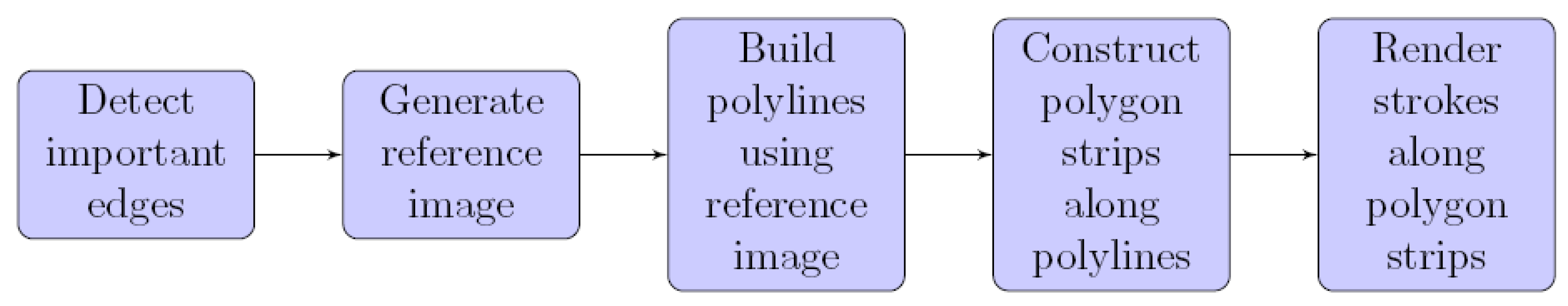
Our algorithm for rendering artistic strokes along 3D silhouettes is designed to mirror the creation process of ukiyo-e prints. Firstly, the ‘important edges’ are detected (silhouettes, creases, and boundaries) [5]. Then, a reference image of the scene is created to determine which edges are visible. The reference image creates a basis for the lines which are rendered in the final image much like the artist’s original design creates the basis for a print. The reference image is then analysed and polylines following the edges visible in the scene built. The creation of these polylines is similar to how the block cutter would cut lines to create a keyblock. Both the polylines and the keyblock are used to impress the shape of the original design onto the final image. Polygon strips are built along the polylines to mirror the inking of the keyblock. Finally, to produce the final image (which corresponds to a print), stroke textures are rendered along the polygon strips. The key steps are illustrated conceptually in Figure 3.
2.1.1. Important Edge Detection
The first step in rendering lines concerns the detection of the important edges in the scene [5]. These can be categorized into three groups: boundary, edges, and silhouette edges that outline objects.
Boundary edges are arguably the simplest type of important edges. These are edges with one or no adjacent faces so there is no connected face to continue the surface. As the name implies, boundary edges mark a boundary where a mesh is discontinued. Creases are defined as edges where the dihedral angle between the two adjacent faces, readily computed by checking if the dot product of the corresponding surface normals is below a certain threshold. Each object in the scene is assigned a crease threshold. The last and the most important edge type is the silhouette edge. These outline the shape of the visible parts of a scene object and are dependent on the current viewpoint: an edge is a silhouette edge if one of its two adjacent faces is front facing and the other is back facing relative to the current viewing position.
The determination of silhouette edges starts by first calculating a viewing vector from the camera optic centre to any point on the edge (one of the end point vertices is used for simplicity). Then, the dot product of the viewing vector with each of the two adjacent face normals is calculated. If the signs of the dot products differ then one face points towards the view while another points away the edge is a silhouette one. Similarly, if one of the dot products is zero then the face is parallel to the viewing vector so the edge should be highlighted. Therefore, if the product of the dot products is less than or equal to zero then the edge is marked as important. Algorithm 1 summarises the process.
| Algorithm 1 Finding important edges |
|
2.1.2. Reference Image
Once the important edges in a scene have been detected, it is still necessary to determine which of these are visible. An edge might be occluded partially or entirely by one of the objects in the scene (including potentially the object which the edge belongs to). Which edges are visible in the scene is determined by rendering them to a reference image. In order that the reference image can be analysed in subsequent stages, it is necessary to be able to identify uniquely each edge in the image. To this end, each edge is assigned a unique colour to be rendered with in the reference image. It is also necessary to ensure that no edge shares a colour with the background colour used to prevent the background being detected as an edge.
To determine visibility, we employ a variation of the technique known as depth buffering [6]. A depth buffer is used to determine which parts of edges should be hidden by rendering the entire mesh of each scene object to fill their interior. The appearance of these meshes does not matter so only their depth values are considered. By rendering these meshes the depth buffer handles hidden lines by not rendering any parts of edges that appear behind the meshes.
One issue which emerges from visibility determination in this manner is that of so-called z-fighting [7]. As the important edges are part of the meshes used to determine visibility, they share the same depth values with the faces on the mesh they are highlighting. Floating point errors introduce inconsistency in ordering creating a “stitching” effect. In the reference image this could cause some parts of edges not to be rendered when they are in fact visible. To address this issue, we apply a small depth offset to the rendered meshes. This offset ensures the object meshes are slightly further from the camera than their corresponding important edges. Therefore, clashing depth values and z-fighting are avoided.
2.1.3. Reference Image Analysis
With the reference image created (see Figure 4), 2D image processing techniques are used to determine how strokes should be rendered in the final image. The goal for this part of the algorithm is to efficiently build polylines that closely match the important lines in the scene described by the reference image. Several constraints are placed on how the polylines are constructed to achieve smooth lines that follow the geometry of objects closely. This process consists of identifying visible edge segments and inferring how they can be linked to one another.
The first step in analysing the reference image consists of identifying the visible edges that appear in the scene. This is achieved by iterating over each pixel in the image and building a set of colours that are present. Each colour represents a unique edge in the image. Therefore, only the edges corresponding to the detected colours need to be considered when analysing the image.
To begin building a polyline, a colour in the set of edge colours in the reference image is chosen. By tracing along where the edge should have been rendered in the reference image, a set of segments in screen space are identified where the edge is visible in the scene; this could be a single segment spanning the full length of the edge if it is completely visible or several segments if it is obscured in one or more places. The process of tracing edges in the reference image and identifying segments is discussed in detail later.
Once the segments are identified, possible links for forming polylines are considered. Edges are joined to other edges at their end points so it makes sense to link only segments that touch the end points of edges. If one of the segment’s end points is also one of the end points of the edge it runs along then there is potential for it to be linked with segments of another edge to form a polyline.
Figure 5 shows examples of segments that could be produced from tracing an edge in the reference image. In Figure 5a the edge is fully visible in the reference image so a single segment is produced from tracing which goes from one end point to the other. As this segment touches both ends, it is a candidate for linking at both end points for building polylines. Figure 5b presents a scenario where both the end points are obscured in the reference image. Tracing the edge results in a single segment that does not touch either end point. As the segment does not touch an end point it cannot be linked to other segments. Therefore, segments like this are immediately added to a list of finished polylines as a single segment. In Figure 5c the edge is partially obscured in its centre so there are two segments, one attached to each end point. Each segment touches an end point so each is a candidate for linking into longer polylines from their corresponding end points. Finally, Figure 5d shows an example of a combination of the previous cases. The edge is obscured in its centre and at an end point so the tracing produces two segments. One segment touches an end point so can be linked into a longer polyline. The other segment does not touch any end points and cannot be linked so forms a single segment polyline.
If there are segments that are candidates for linking then the links are followed to build polylines until the segments can be linked no further. The process of linking begins with identifying an edge that could be linked to the segment’s end point and its colour. How an edge is chosen as a valid link is discussed in detail later. The chosen link edge is traced in the reference image as before to find visible segments. If one of the new segments shares an end point with the original then a polyline is created consisting of both segments. If the new edge traced was entirely visible such that the segment touches both end points then the process of linking can be continued from its other end point to build an even longer polyline. If the target link edge is not entirely visible and segments do not touch the necessary end point then they cannot be linked and are placed in separate polylines. Even if the edges cannot be linked, if the other end point of the target link edge is touched by a segment then linking can continue from that segment with a new polyline. This process is repeated and edge segments are linked until there are either no more valid links to follow or segments of the target link edge do not touch the next end point.
Once no more links can be created, the finished polylines are stored and the entire process begins again by choosing a new colour from the set of reference image colours. During the process of building polylines, the colour of each edge used in a polyline is recorded to ensure that none are ever used twice. Once all the edge colours from the reference image are used in a polyline the analysis of the reference image is complete.
2.1.4. Segment Identification
For a given edge, the first step in identifying visible segments in a reference image is finding where in screen space the edge should be. The position of the edge’s end vertices are converted to screen space as they would be when the edge was rendered. The line between these end points is traced in the reference image using a variation of Bresenham’s line drawing algorithm [1]. While being traced, segments are formed where the edge is visible (where pixels use its colour). The algorithm functions by evaluating the slope of the line described by two end points. First, the dominant axis is determined by comparing the endpoints and . The dominant axis is the one which differs the most between end points:
If is larger than then x is the dominant axis and vice versa. The line drawing begins at the pixel the first end point lies in. At each step a new pixel is drawn to. The position on the dominant axis always moves one towards the other end point at each step. The position on the non-dominant axis either stays the same or moves one towards the end point based on the current error value.
The error value begins at 0 and is incremented at each step by . When the error exceeds 0.5 then the position on the non-dominant axis is moved closer to the end-point, otherwise it stays the same.
While normally used for rendering lines, here the algorithm is utilised to trace the pixels that an edge should cover in the reference image. While tracing the line, the first pixel encountered of the target edge colour is marked as the start of a segment. The line is traced until a pixel is encountered that does not use the edge colour at which point the end of the segment is marked. The tracing continues creating new segments until the end of the line is reached. The segments are defined by the pixel coordinates of the first and last traced pixel that used the edge colour. The only exception to this is segments that touch the first or last pixel in the traced line. In this case the actual target end points originally calculated are used for those points in the segments. These segments that touch the line end points are also marked to be considered for linking in other parts of the line rendering process.
Any segments traced that only cover one pixel are discarded as at least two points are required to define a segment. The only exception to this is when the entire line traced is just a single pixel. In this case the original target end points can be used for the segment instead of the pixel coordinates enabling a full segment to be defined. As the line tracing cannot guarantee to perfectly trace the rendered edge, the algorithm was modified to introduce some leniency. This comes in the form of two parameters that alter which pixels are searched and how segments are formed.
The first parameter is the search width. This checks additional pixels on either side of the line traced. For example, a search width of two will search two extra pixels on either side of the current pixel when tracing. If any of the five checked pixels contain the target edge colour then the current segment can be continued. For simplicity, these extra pixels searched are not perpendicular to the line but instead are perpendicular to the dominant axis of the line being traced. While this is slightly less accurate, most of the time it is equivalent and is cheaper to calculate.
The second parameter is a valid number of misses when building a segment. Rather than finishing a segment on the first pixel encountered which does not match the target colour, n successive steps of the tracing must be passed without encountering the edge colour before the segment is finished where n is the maximum misses. This is also applied to the start segment, if any of the first n steps encounter the edge colour then the first segment is considered to be connected to the start end point and so can be linked from it. Similarly, if the last segment traced reaches the end of the line before there are n misses in a row then it is counted as connected to the end point even if the last pixel checked was a miss. This miss value n must be chosen carefully as if it is too large it could result in areas where the edge is obscured being ignored. Choosing a good number of misses is discussed in further detail in the evaluation section.
2.1.5. Linking Segments
The strategy used for linking segments is quite different from the algorithm the line rendering process is based on. The algorithm described by Northrup and Markosian [8] forms polylines by first finding the visible segments for all edges in the reference image. Some unnecessary segments are removed such as overlapping parallel segments being joined into a single segment. Then, these segments are compared in order to link them using a set of rules based on the angle between the segments and pixel colours that appear near their end points. This strategy for linking only considers how appropriate it is to link segments in the 2D reference image. This does not consider the depth of the scene so two edges that are very far apart in world space could end up being linked in a stroke. This can result in strokes that do not accurately follow the shape of individual objects. Furthermore, without considering the geometry of objects in the scene it is difficult to consistently make the same links in consecutive frames leading to poor temporal coherence.
The strategy proposed in this work for linking segments seeks to match the geometry of objects in the scene as closely as possible. In scenes with multiple objects, it makes sure that links are never made to edges on separate objects to make sure the final image is visually coherent. The linking ensures that the strokes describe the shape of object clearly and links are consistent between frames to maintain temporal coherence. This strategy uses a graph which describes how edges and vertices are connected in each mesh. The search for potential links begins with the vertex that is the end point of the segment to be linked. The mesh graph is searched to find edges which use that vertex as an end point. If one of the edges has its corresponding colour in the reference image and has not already been used in another polyline then it could potentially be used as a link.
Before a chosen link is used for tracing to find segments for use in a polyline, another check is carried out to ensure it would be appropriate to join these edges in a stroke. To avoid creating jagged, unappealing strokes in the final image, an edge is only chosen as a valid link if the difference in direction with the target edge is below a certain threshold. If the angle between the edges is greater than the maximum allowed link angle for that object then it is not chosen as a link. The list of edges connected to the target vertex are searched until one is found to be a valid link or no more edges remain. A chosen edge is then traced to find segments so that they can form polylines with the previous segment if possible as discussed earlier.
An issue with this strategy is that when objects are distant from the view or the resolution is low, every single important edge might not be rendered. For example if a model is very detailed with many small edges then only every second connected edge might be visible due to not enough pixels to render all of them. In these scenarios, only checking directly connected edges in the mesh graph is not sufficient. A search depth parameter is set dictating how deep into the edge graph should be searched for finding valid links. If no valid links are found directly connected to the target vertex then the next depth is searched checking all edges connected to the edges in the initial search. This breadth first search of the graph continues until a valid link is found or the search depth limit is reached. As depth increases, the search can become increasingly expensive. To try and keep the search cheap, which edges are explored in the graph are constrained. Edges are never followed deeper in the search if they have been used in another polyline or have already been visited in the search. Furthermore, only edges that are marked as important edges are followed deeper into the search. If a potential link is found at the current depth but it is rejected due to the angle between the edges then the search will not go any further than the current depth. It is not a requirement that the edges followed are in the reference image, merely that they were marked as important at the start of the rendering process. This allows the search to bypass important edges that do not appear in the reference image due to its resolution.
2.1.6. Rendering Strokes
Once the polylines describing the scene have been created, the final step is to render strokes along these lines. This process consists of building polygon strips along the path of each polyline and then rendering a stroke texture along the strips. This results in strokes rendered in 2D capturing the 3D structure of the scene.
The method for building strips is based on a strategy previously used for creating artistic silhouettes [8]. A “rib” is formed at each vertex in the polyline. Consecutive ribs are joined with polygons to form a long path that a stroke texture can be rendered along.
The length of each rib is dictated by a stroke width parameter. Ribs are formed at the vertices which are end points for a polyline by creating a vector perpendicular to the vector from that vertex to the only connected vertex. At vertices that lie between two segments the rib direction is perpendicular to the direction from the previous vertex to the next vertex. For example, a rib at vector which lies between vertices and vi+1 in a polyline is perpendicular to the vector defined by .
To ensure that the width of the full path is consistent, ribs that are on a corner between two segments must be scaled up. The width scaling factor for these ribs can be calculated as:
where is the rib vector at vertex and is the unit vector perpendicular to . This causes ribs to be scaled wider at sharper corners. Furthermore, to prevent excessive scaling at very sharp corners a scale limit parameter is defined which caps the size of the scaling factor.
It is possible that some polylines have a total length that does not span more than one or two pixels. Such lines might not look aesthetically pleasing when rendered. Short polylines result in a squashed stoke that does not resemble the long strokes desired. As a result, an extra minimum length parameter was added to filter short polylines. Any polylines with a total length less than the minimum are discarded before strips would be built for that line. A typical final result is shown in Figure 6.
2.1.7. Reference Image Optimisation
The analysis of the reference image can become a performance bottleneck, especially at larger resolutions. As the resolution increases so does the number of pixels that must be iterated over when building the set of visible colours. Identifying segments also becomes more costly as edges cover more pixels.
A strategy for optimising the reference image analysis was inspired by methods for optimising shadow mapping [9] i.e., by creating a “shadow map” that is the scene viewed from the perspective of the light source. When rendering the final image, depth values are compared with the shadow map to determine which areas are in shadow. The resolution of the shadow map can be decreased to less than the final image’s resolution to improve performance but decrease shadow quality. A lower resolution shadow map is cheaper to compute but results in poorer shadow quality.
The function of the shadow map is similar to how the reference image is used in the line rendering algorithm. They both involve creating additional images to aid in the rendering of the final image. Just as the resolution of the shadow map can be decreased, the resolution of the reference image can be decreased to reduce the cost of the analysis stage. As discussed earlier, lower resolutions can lead to missing edges in the reference image. By increasing the search depth parameters for finding links, the issues of a smaller resolution can be alleviated and in many case the difference in strokes formed is negligible. This is investigated further in the evaluation section.
Decreasing the resolution of the reference image does not alter the resolution of the final image. It just affects how accurately the reference image represents the scene. However, decreasing the reference image resolution does mean that the polylines created from analysis will be in screen space for that resolution. Therefore, when polygon strips are created, their positions must be scaled up to fit the resolution of the final image. It is even possible to increase the resolution of the reference image larger than the final image to improve the precision of analysis at the cost of a more expensive analysis. This could be practical when the final image uses a low resolution.
2.2. Colour
While earlier prints were solely defined by black ink lines, once coloured inks and dyes became readily available, the vivid colours ukiyo-e is known for became common place. In the initial design artists would mark parts of the design to be filled with different colours. When passed to the block cutter, a wood block would be cut for each section which required colour. For each coloured area, the printer would take the corresponding block, spread a dye across the block, and press the correct area of the paper onto it with the baren. There were many subtleties to the printer’s process that could create special effects which often increased the appeal of the print.
This section details algorithms for rendering objects with a variety of colouring techniques used in ukiyo-e prints. This includes textured prints and the bokashi effect for gradation of colours. Close attention was payed to the ukiyo-e printing techniques in the design process to try and create authentic looking images. In particular, the algorithms in this section attempt to maintain the 2D look of ukiyo-e prints while maintaining temporal coherence in a 3D environment.
2.2.1. Pseudo-Uniform Colours
The simplest use of colours in ukiyo-e prints involved the use of uniform, vibrant colours. The printer would spread colour evenly across the printing block to impress onto the paper. However, multiple factors influenced how the colour appeared on the paper often resulting in an inconsistent pigment across the coloured area. The inconsistency could be a result of slight differences in the concentration of dye across the printing block. Depending how evenly the printer presses the baren on different parts of the block, the dye could be absorbed more at different points on the paper. Furthermore, the surface of the wood block was rarely perfectly flat and the texture of the wood often influenced how colour was impressed onto the paper. The fading of different types of dyes over time could also influence the consistency of colours in a print which is why many prints that still survive lack the vibrant colour they once had.
While completely uniform colours are simple to render for the body of a mesh, the colour in ukiyo-e prints features inconsistency which we model by purposeful introduction of additive noise texture. Normally in 3D rendering, textures are mapped onto 3D meshes so as to avoid the appearance of projection artefacts. However, given that the aim in the present work is to mimic the appearance of ukiyo-e printing, the noise texture should be done in the 2D screen space, rather than the 3D world space. Hence, rather than using predefined texture coordinates at each vertex, the texture coordinates are based on the model’s position in screen space. Once a primitive that is part of the mesh has been rasterized, each pixel determines which part of the corresponding noise texture to use based on their screen coordinates:
where and are the screen space pixel coordinates and and the dimensions of the noise texture. The modulo operation ensures the texture coordinates are within the correct boundaries, effecting repetition when covering large areas. Therefore, to achieve perceptually best results, noise textures herein should exhibit looping, cyclic behaviour. The final colour of the pixel is computed by combining the colour at the calculated texture coordinate with the target colour for that scene object. This results in the object being coloured with the target colour with imperfections introduced by the noise texture; see Figure 7.
While rendering with a noise texture is effective for creating still images, it creates poor temporal coherence when the scene is in motion. The noise texture’s position only depends on screen position of pixels and not the object’s position so when an object moves in the view it appears to “swim” through the noise texture behind it (so-called “shower door” effect). So that the noise texture follows the object as it moves in the scene, the original calculation for texture coordinates was modified. First, an offset based on the object’s position is added so that the noise texture follows the object as it moves left, right, up and down relative to the view. A centre point is defined for each object in the scene from which to calculate the offset. For simplicity, the origin in model space can be used as the offset but it can also be appropriate to define custom centres for some meshes. The centre point’s position in screen space is used as the offset. Each pixel adds the offset when calculating texture coordinates to account for the position of the object in screen space. The depth of and scaling of the object must also be considered so that the scale of the noise texture matches the object as it moves away or towards the view position. Therefore, the noise texture is scaled based on the depth of the centre position from the viewing position. The modified calculation for texture coordinates at each pixel is as follows:
where and are the screen space coordinates of the object’s centre and d is the object depth.
2.2.2. Texture Application
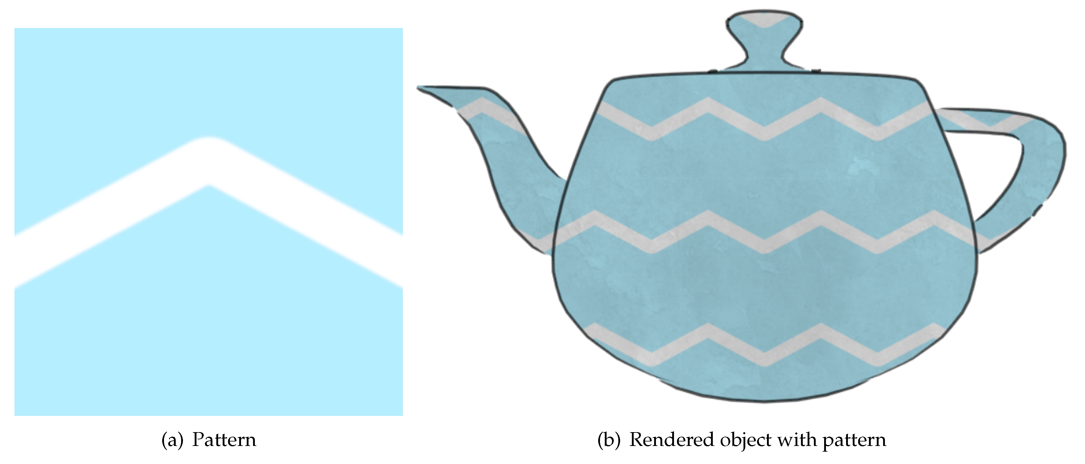
Over time ukiyo-e artists would begun to include patterns in their designs (e.g., when depicting clothing, see Figure 8) rather than just uniform colour. We adapt our previous algorithm for mimicking simple uniform colouring for emulating the more complicated textures.
To maintain the style of ukiyo-e, the same strategy used for the noise textures was used for adding patterns with pattern textures used in a manner similar to how previously noise textures were applied. Specifically, screen coordinates and an offset were used to calculate the texture coordinates for each relevant pixel. Instead of combining the noise texture with a uniform colour, now the former is added to the corresponding pattern texture. Figure 9 exemplifies the result.
2.2.3. Bokashi
One of the most recognisable effects in ukiyo-e prints is the gradation of colour created using a technique called bokashi [4]. This effect was created by a printer by first moistening the wood block to be used for the gradated colour. Spots of the colour to be used were placed around the edge of the block where the colour was supposed to be at its most intense. Then the printer would use a brush to spread it out across the rest of the block to create a gradual dilution of the ink or dye. Finally, printing would be performed by resting the paper on the block and pressing it with a baren.
Inconsistencies in the spreading of ink on the block and the fact that the printer could not see the print while pressing the paper onto the wood blocks mean that colours and gradation do not accurately follow the shape of objects like in conventional paintings. The gradation of colour in ukiyo-e prints usually gives an approximation of lighting, shape, and depth while the line work captures the actual detail. As a result, shading strategies which accurately follow the shape of objects such as cel shading [2] are inappropriate; hence, we developed two different algorithms for emulating the bokashi effect. The first of these mirrors the physical printing process whereas the second is in spirit closer to more traditional 3D shading strategies.
Bokashi Algorithm 1
Our first algorithm is based around creating a linear gradation of colour in screen space to mimic a 2D print. It uses a central point on each object to determine how greatly the light is acting upon that object. Then, based on the strength of the light it creates a linear gradation of colour across the object towards the light source. The centre point is defined similarly to the centre point used for textures. It can be the origin in model space or another point that better represents the centre of the object. A light is defined by a position and its strength. Using the light and the centre position, a gradation point is calculated. The line perpendicular to the vector from the light at the gradation point determines the border between between the illuminated and unilluminated halves of the object for the purpose of gradation. The gradation point g is calculated as follows:
where c is the centre position of the object in world space, s is the light strength, and d is the light ray direction. The parameters and o are characteristic for an object and describe how easily the object is illuminated, the former being a modifier for the light strength at the centre of the object, and the latter representing the length of an offset from the centre that the default gradation point is. A negative offset means the gradation point starts closer to the light and the object is less illuminated while a positive offset causes the object to be more illuminated by default.When an object is rendered, each pixel calculates its colour based on its position relative to the gradation position and the light direction in screen space. To calculate the colour for a pixel, the vector from the gradation point to its coordinates is calculated. The size of the vector in the light direction is calculated to determine which side of the gradation boundary the point lies and how far from the boundary it is. Our algorithm takes into the viewing position to improve temporal coherence. As the viewing position moves towards a position where the object lies directly between it and the light then the object should appear less illuminated. Similarly if the view position is close to light ray then the portion of the object visible should be more illuminated. To this end, a view modifier m is applied:
where v is the view vector from the viewing position to the object centre point in world space, l is the vector from the light position to the centre point in world space, is a base view modifier value that is defined for each object, and the modifier denotes normalization. The gradation position in screen space is moved by the light direction in screen space scaled by m. When the view vector is perpendicular to the light vector then m is zero so the gradation position is not modified. When the object is between the view and the light source then the modifier is negative and the gradation point is moved close to the light resulting in the unilluminated portion of the object being larger. Similarly, if the view position is on the side of the light relative to the object then the modifier is positive and the gradation position is moved further from the light resulting in a larger illuminated area. This modification helps to give the object a more 3D feel while maintaining the 2D gradation of colour.
Our basic algorithm was further modified to improve temporal coherence as the depth of the object varies. The rate modifier and view modifier are scaled based on the depth of the centre point into the scene from the view position. This causes more distant objects to have larger gradation rates so gradation is completed over a smaller distance and view modifiers are decreased so that the additional offset is smaller. Similarly, closer objects have a more gradual gradation and the view modifier offset is larger. Overall, this makes gradation rate and position alter to match the distance of the object and thereby improve temporal coherence when changing depth. As with the previous colour rendering algorithms, this strategy is combined with a noise texture. Figure 10 shows the result of applying the algorithm on an example object.
Bokashi Algorithm 2
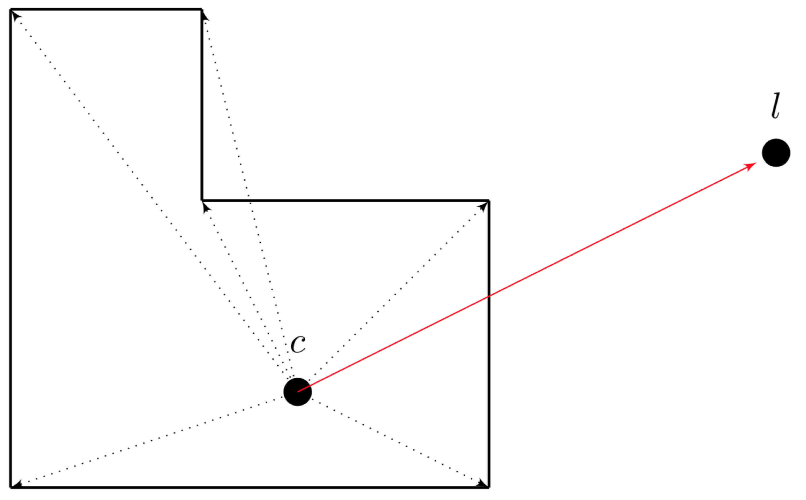
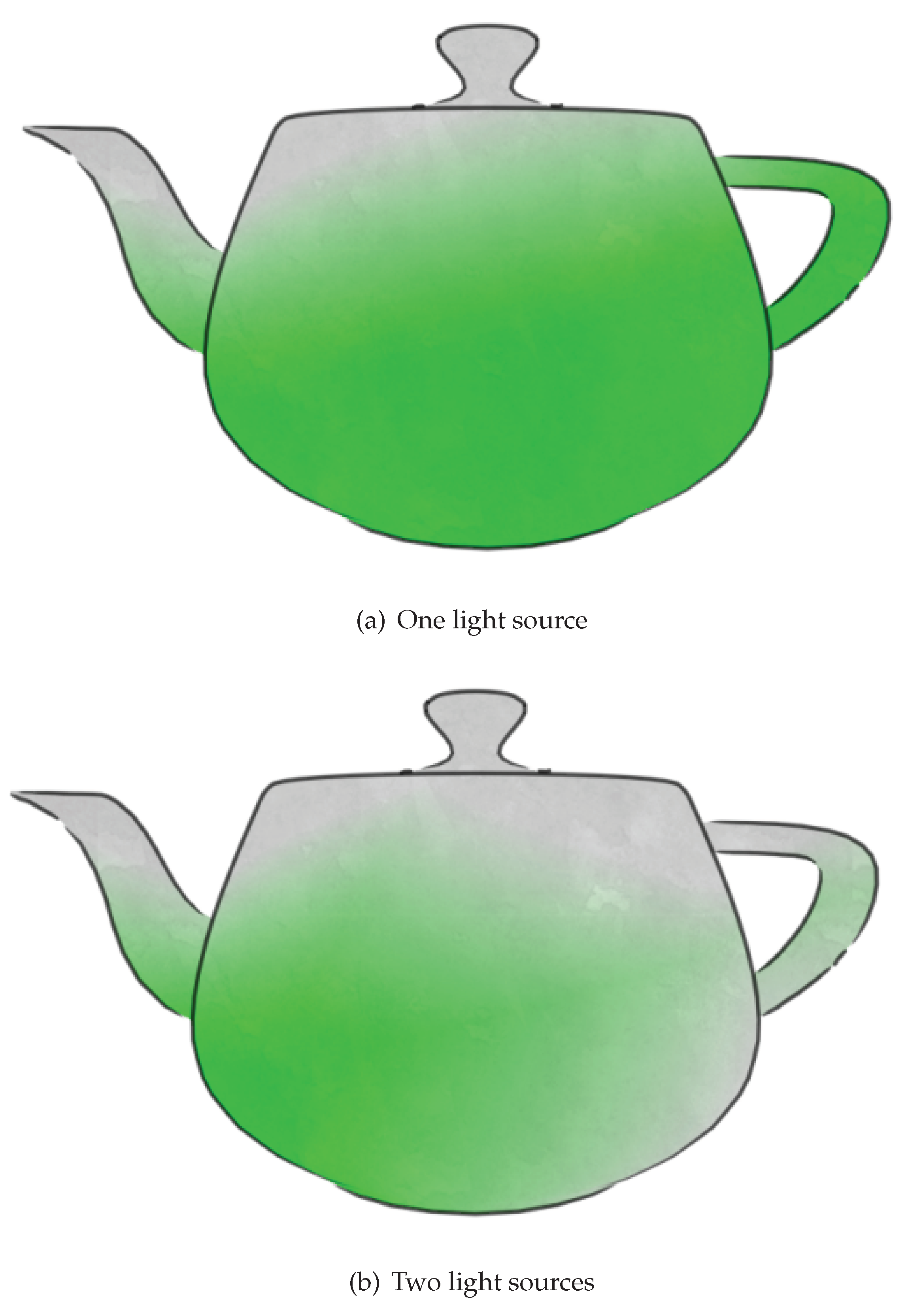
The second approach to emulating the bokashi effect was based on more traditional 3D shading strategies [10,11]. However, while these attempt to create realistic lighting effects our method achieves the more artistic style of gradation in ukiyo-e. To achieve a smooth gradation in scene objects regardless of their shape, they are treated as spheres for the purpose of shading. When a sphere is illuminated there is a linear gradation from light to dark from the point closest to the light to the point furthest from the light. Therefore, if the shape of an object can be approximated as a sphere then it can be shaded with standard shading models like Gouraud or Phong to achieve a linear gradation of colour across the surface. The shading calculation used is the same but our method uses a different way of determining the vertex normals and light vectors. As previously, a centre point is defined for each object, used as an infinitesimal sphere, the shading of which if used to approximate the shading of the object. Instead of using predefined vertex normals, the normals used in shading calculations are calculated as the unit vector from the centre point to the vertex being shaded. Furthermore, the light ray used is not the vector from the vertex to the light as would be used in Gouraud or Phong shading but rather the vector from the centre point to the light locus, causing each vertex to represent a point on the central sphere when shading calculations are carried out. Figure 11 describes in 2D the calculation of surface normals for an object from a centre point c. Furthermore, the red line from the centre to the light position l describes the light vector used for all shading calculations for that object.
This strategy can be used as a variation of Gouraud or Phong shading. For a variation on Gouraud shading, the shading factor f is calculated at each vertex as follows:
where n is the normal vector from the centre to the vertex and d is the light vector from the centre to the light position. s is the strength of the light and is scaled with the inverse distance to the centre so as to modify the shading factor depending on how strong the light at the centre point is. Shading factors are constrained to the value range from 0 and 1. The shading factor describes how illuminated the vertex is where 0 is not illuminated and 1 is fully illuminated. Interpolation across faces is performed as a means of quickly computing the factor for each pixel. If Phong shading is to be used instead, the only difference is that the calculation of f is carried out at each pixel. The value of n in the Phong version is the interpolated unit normal calculated at each vertex on the face the 3D that corresponds to a pixel of interest lies on. Multiple light sources are treated seamlessly, simply by aggregating shading factors for all sources, and then imposing the constraint on its value begin between 0 and 1. This process can be used to create more complicated gradation effects. Figure 12 shows examples of an object shaded using the Phong variation of our shading model. The shading is combined with a noise texture like before, so as to mimic physical imperfections of the printing process in the real world.
3. Evaluation
The proposed framework and algorithms were evaluated using numerous test scenes. Representative example results are shown in Figure 13. The image in Figure 13a shows a scene composed of multiple boxes, each rendered using a different shading strategy: the green cube uses the sphere based bokashi algorithm, the tall box at the back uses the first bokashi algorithm, and the last box is decorated with a pattern. The scene in Figure 13b depicts a magnolia flower rendered using our sphere based bokashi algorithm, as do the scenes in Figure 13c,d. Finally, the scene in Figure 13e shows a trumpet rendered with a pseudo-uniform colour. All models used in the scenes are freely available from online sources (see https://groups.csail.mit.edu/graphics/classes/6.837/F03/models/, and http://people.sc.fsu.edu/~jburkardt/data/obj/obj.html) and the examples shown chosen for their varying degree of complexity, both in terms of the number of polygons (see the summary in Table 1) and the nature of the shapes.
3.1. Performance
Our performance analysis involved the measurement of the average frame rate of the scene in the rendering environment. The frame rate was averaged over a 30 s period of the user manipulating a scene. As discussed in greater detail shortly, the performance can depend on the viewing angle so the view of the scene was kept static for duration of the measurement period. Experiments were carried out on a PC with a four core 2.9 GHz Intel Core i5-3470S processor and integrated graphics. Unless otherwise specified, the window resolution used in experiments was 720p ( pixels). Furthermore, as some of the stroke parameters directly affect how much work is done, unless otherwise specified the line rendering parameters were kept constant throughout experiments. In particular, the resolution of the reference image was the same as the window (720p), a search width of 2 was used for the line tracing and a link depth of 3 was used for searching for edges when linking.
3.2. Main Results
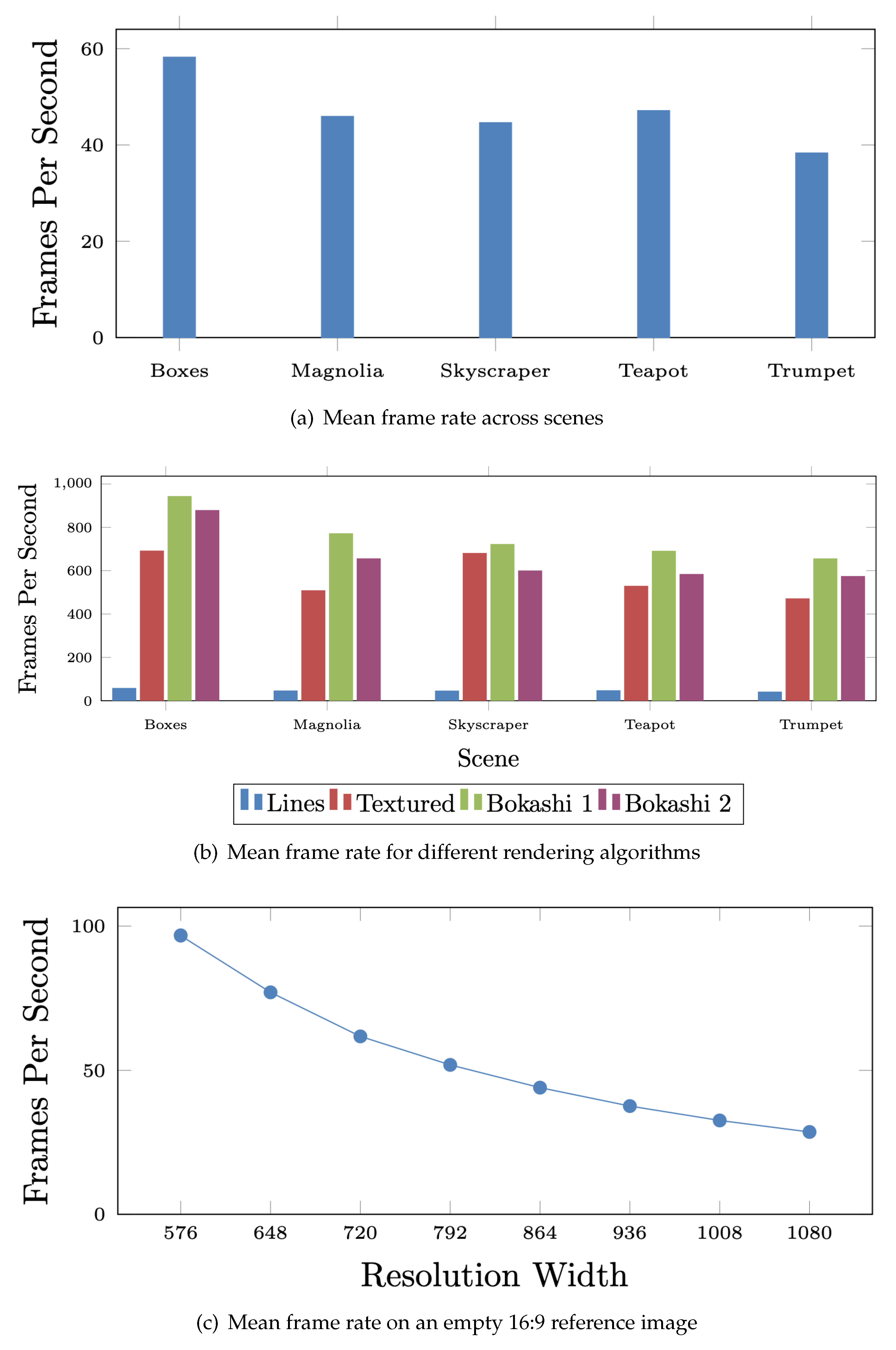
We firstly sought to gain a general insight into the performance of our algorithms by measuring the average frame rate of each of the example scenes. Figure 14a shows the results, ordered by the polygon count. In all instances an interactive frame rate above 30 fps was achieved. Interestingly, these results show that the polygon count does not appear to be the most influential factor when it comes to processing performance. For example, the teapot scene which has almost twice as many polygons as the tower/skyscraper was rendered at a higher frame rate.
To investigate the effect on performance of each individual algorithm, the average frame rate of each scene was measured again when rendered with only one of the algorithms. Each scene was rendered once for lines, textures, and each of the bokashi algorithms. For example, to measure performance of the first bokashi algorithm on a scene, each object in the scene was shaded with that algorithm and none of the other rendering strategies were applied (such as the line rendering algorithm). This isolates each algorithm and gives an indication of the individual effect on performance. Figure 14b shows the results of this experiment. Each of the shading and colour rendering strategies easily achieve interactive frame rates. Furthermore, the burden of colour rendering algorithms scales linearly with the number of polygons as expected from their design. The line rendering frame rates measured in this experiment using just the line algorithm are almost identical to the frame rates in the initial experiment results displayed in Figure 14a which shows that the line rendering algorithm is a performance bottleneck.
The colour rendering techniques allow high data parallelism which permits them to be almost entirely implemented to run on the GPU. While rendering, the reference image and the final strokes in the line rendering algorithm can exploit the GPU to accelerate rendering, the analysis of the reference image and building of the polylines takes place on the CPU and the cost of this is the limiting factor in performance of the ukiyo-e rendering process. The cost of the reference image analysis is not primarily based on the number of polygons in the scene. The analysis evaluates the 2D image described by the reference image so ultimately it is the resolution of the image dictates the cost. Tracing edges in the reference image increases in cost as the resolution increases. The initial iteration through the image to find visible colours also increases with resolution. Polygon count is still a factor as more linking must be done if there are more separate lines on screen. However, the associated computational burden increase is not as significant as that of increasing resolution. This is why the first set of results we presented resulted in similar frame rates across scenes despite large differences in polygon count.
To demonstrate the base cost of the analysis based on the resolution, an empty scene was rendered at various 16:9 resolutions. Despite the scene being empty, the line rendering algorithm still iterates through the pixels in the reference image to check which colours are visible. Only once it has checked every pixel does it conclude that there are no visible lines. Figure 14c shows the average frame rate of rendering an empty scene from resolutions from 576p up to 1080p. Before any edge tracing or stroke rendering takes place, the frame rate has already been limited by this initial analysis. At a resolution of 576p, the frame rate is limited to just under 100 fps, while at 1080p the frame rate is just under 30 fps before any additional analysis takes place. Fortunately, the initial pass does reduce the complexity of the subsequent analysis. Without it, each non-visible important edge would need to be fully traced to confirm it was not there which would become extremely costly in more complicated scenes. However, the subsequent analysis still has a cost which is why in the original experiment results some of the scenes exhibited a frame rate considerably lower than the initial 60 fps limit for 720p.
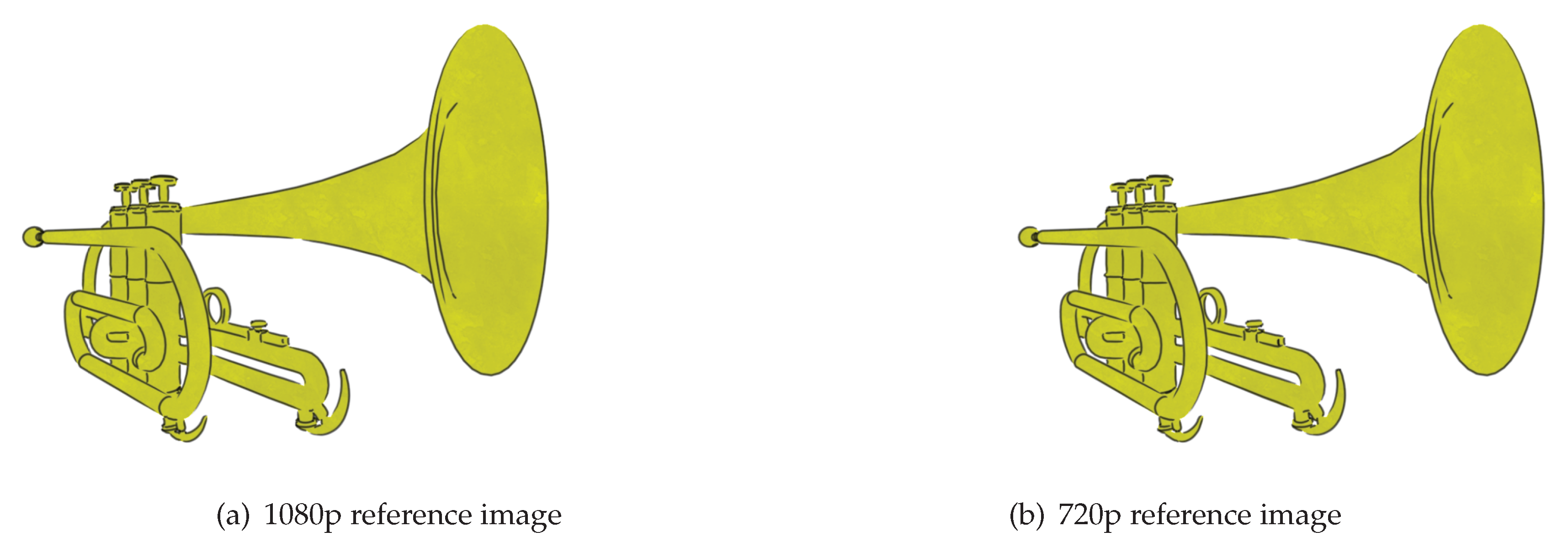
The computational cost of the analysis step can make it difficult to achieve interactive frame rates at high definition resolutions. As discussed previously, the resolution of the reference image can be altered independently of the final image to reduce the overall cost of analysis. The reference image does not need as much detail as the final image. Therefore, resolution of the reference image can be reduced independently of the final image to reduce the cost of analysis. Figure 15 compares a 1080p image of a trumpet with different reference image resolutions. The images look almost identical with similar lines in each. The scene depicted in Figure 15b achieves 40 frames per second by using a 720p reference image compared to 22 frames per second achieved in Figure 15a which uses a 1080p reference image. Adjusting the link depth parameter at different depths can ensure the same strokes are formed. However, if the resolution of the reference image is reduced too much then some finer details in the image can be lost regardless of parameters. Increased link depth does come with some cost but it is insignificant compared to the resolution of the reference image.
Increasing the search width when tracing edges also increases the cost of the analysis. However, a search width of 1 or 2 is almost always sufficient, especially when the line width in the reference image is increased. Using a small search width usually does not create a significant change in performance but can improve stroke quality.
3.3. Temporal Coherence and Image Quality
For the scene to be interactive, the output of a rendering algorithm needs to appear (i.e., perceptually be) coherent between frames. The performance of our algorithms in this regard is discussed in the present section, with highlights on their strengths as well as weaknesses. Factors affecting the quality of created images are considered herein too.
3.3.1. Linear Features
As an object becomes more distant, fewer directly connected edges are visible in the reference image. When only linking directly to connected edges, this can cause strokes to break up the further away they are creating poor temporal coherence as depth varies. Fortunately, the link depth parameter can help to improve linking important edges of more distant objects. Figure 16 compares a distant object with different depths used for searching the edge graph to link edges. Figure 16a shows lines rendered with link depth one so only directly connected edges in the edge graph are considered for linking. This results in fragmented lines as links cannot be found due to the lower detail that the object is rendered with in the reference image at this distance. Figure 16b improves the image by using a link depth of 3. By searching deeper into the edge graph, more links are found, creating smooth linking of lines. The increased link depth comes at marginal computational cost owing to our algorithm only following important edges in the mesh graph. A good choice of link depth allows lines to be linked consistently as an object’s distance from the view varies, maintaining temporal perceptual coherence. Lower reference image resolution can have a similar effect on edge linking so an increased link depth also effects an improvement in this regard.
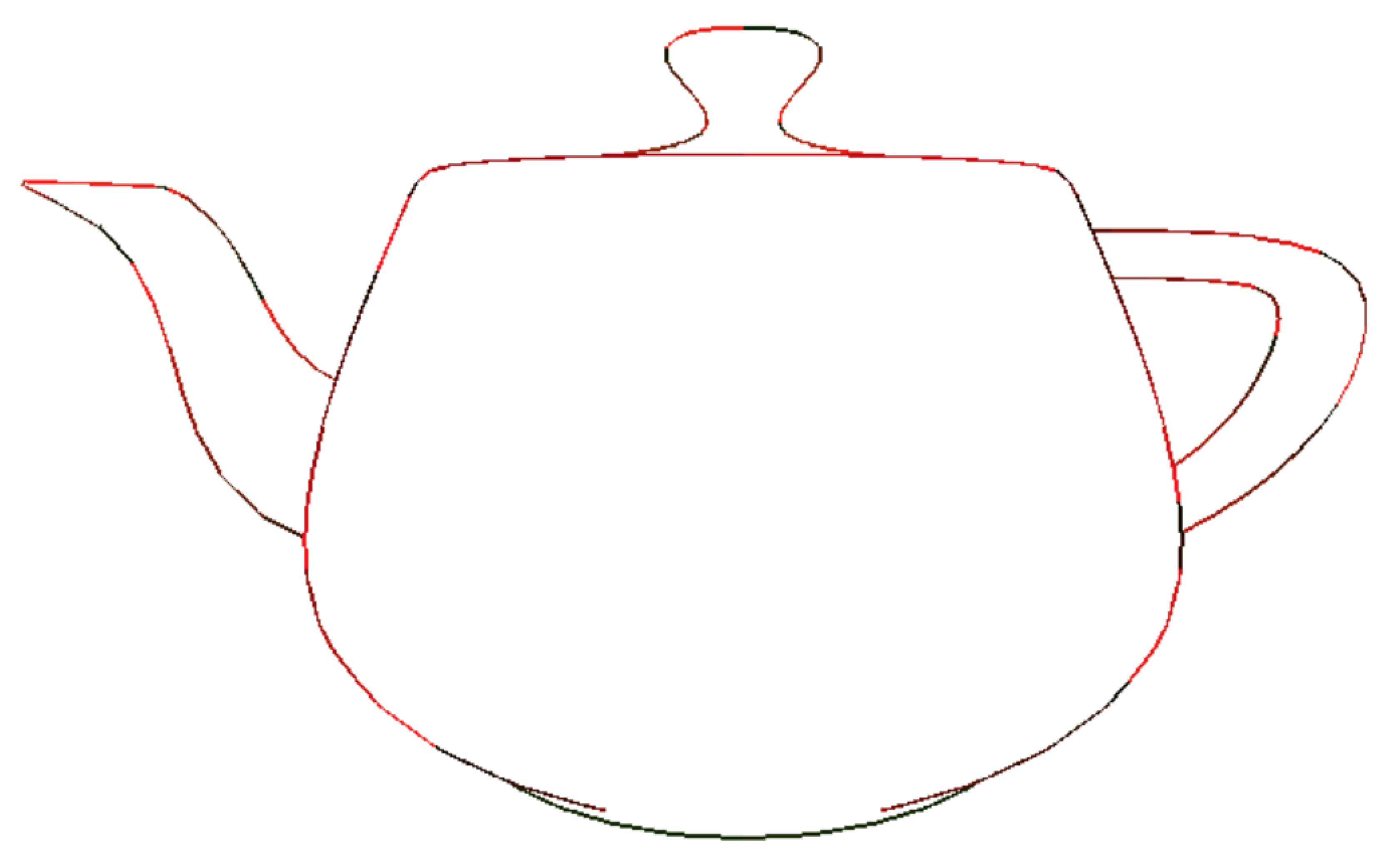
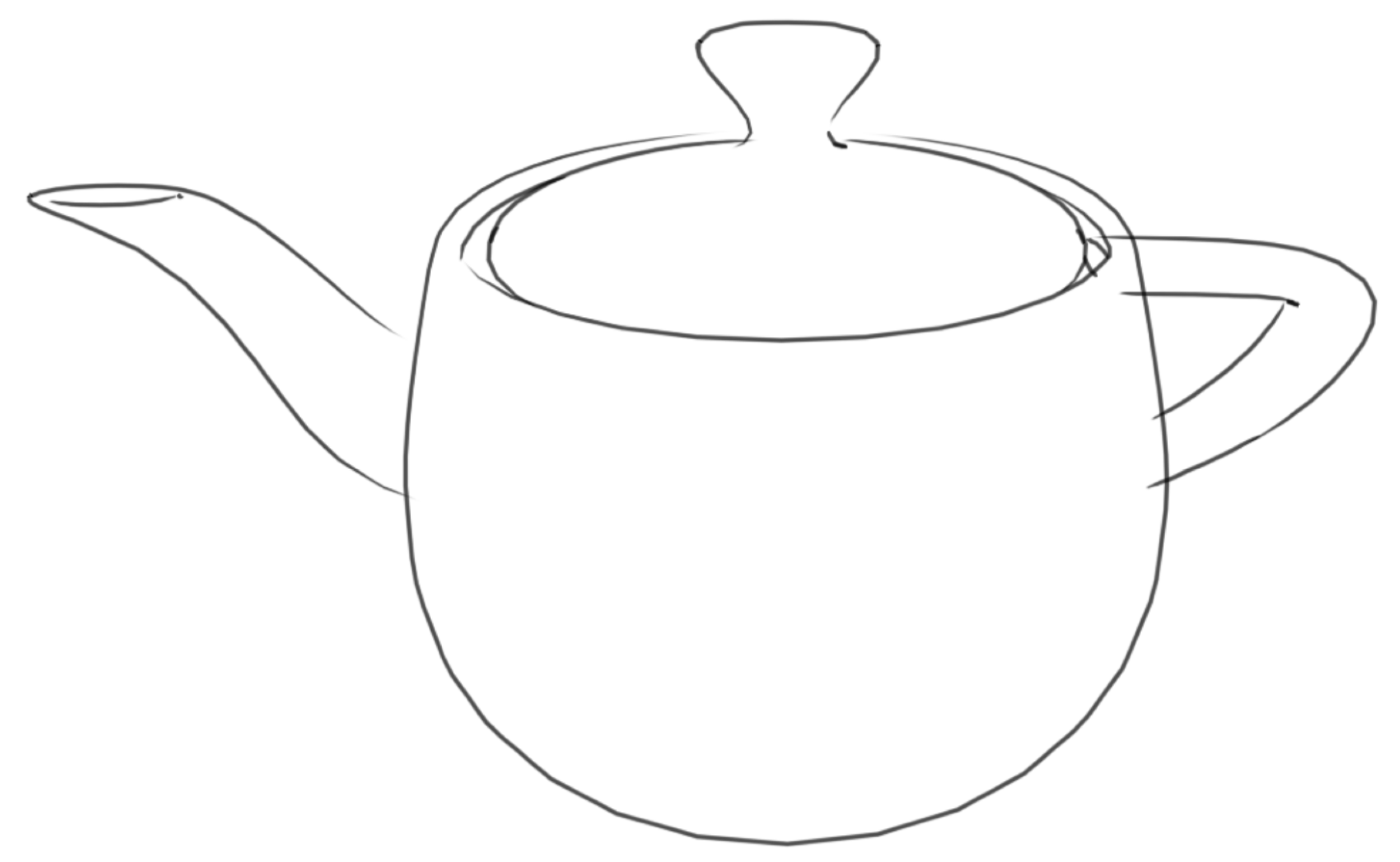
The parameters determining how edges are traced to find segments can also affect image quality. In particular, if the number of maximum misses permitted when tracing segments is too high then parts of obscured edges can end up being rendered (which is clearly an unwanted behaviour). This is a result of the tracing being too lenient in a manner of speaking. Figure 17 demonstrates rendering errors that can arise if the number of misses allowed is too high (the example shows allows thirty misses). It is particularly clear at the teapot handle where some lines should be obscured but are not due to the leniency of the tracing. This creates poor temporal coherence as the segments in lines are coarser and less precise compared to the reference image. Therefore, for the best results, the maximum misses values must be chosen which accounts for imperfections in line tracing but is not too large that it creates segments for obscured parts of edges. The resolution must also be considered as at larger resolutions more misses could be acceptable to create better quality edge segments. In our experiments, up to two misses in a row was found to be an effective value at 720p and similar resolutions, as can be observed in the shown test scenes.
3.3.2. Textures
Due to the 2D nature of the rendering strategy for noise and pattern textures, it was difficult to maintain temporal coherence in all scenarios. The algorithm was designed to deal with change in depth and have the texture follow the object as it moves around the screen. While it accounts for the translation of the object, it does not account for rotation of the object. This was partially by design as the pattern should be “printed” in 2D with the same orientation in each frame to mimic the flat designs in ukiyo-e prints. Furthermore, the texture cannot just be rotated with the object as there are fewer axes of rotation for the 2D texture than in the 3D plane the object exists in. The lack of rotation is less noticeable when the axis of rotation is perpendicular to the vector from the view. However, The lack of rotation is quite noticeable when rotating around the vector from the viewing position to the object as the texture stays static while the object rotates around it. The inconsistency is less obvious with something like a faint noise texture in the background but is more concerning when using a detailed pattern texture. Therefore, while the algorithm can move and scale the texture to approximate 3D translation while maintaining a 2D appearance, it is less appropriate when a large amount of 3D rotation is required along axes with similar direction to the view vector.
3.3.3. Bokashi Algorithm 1
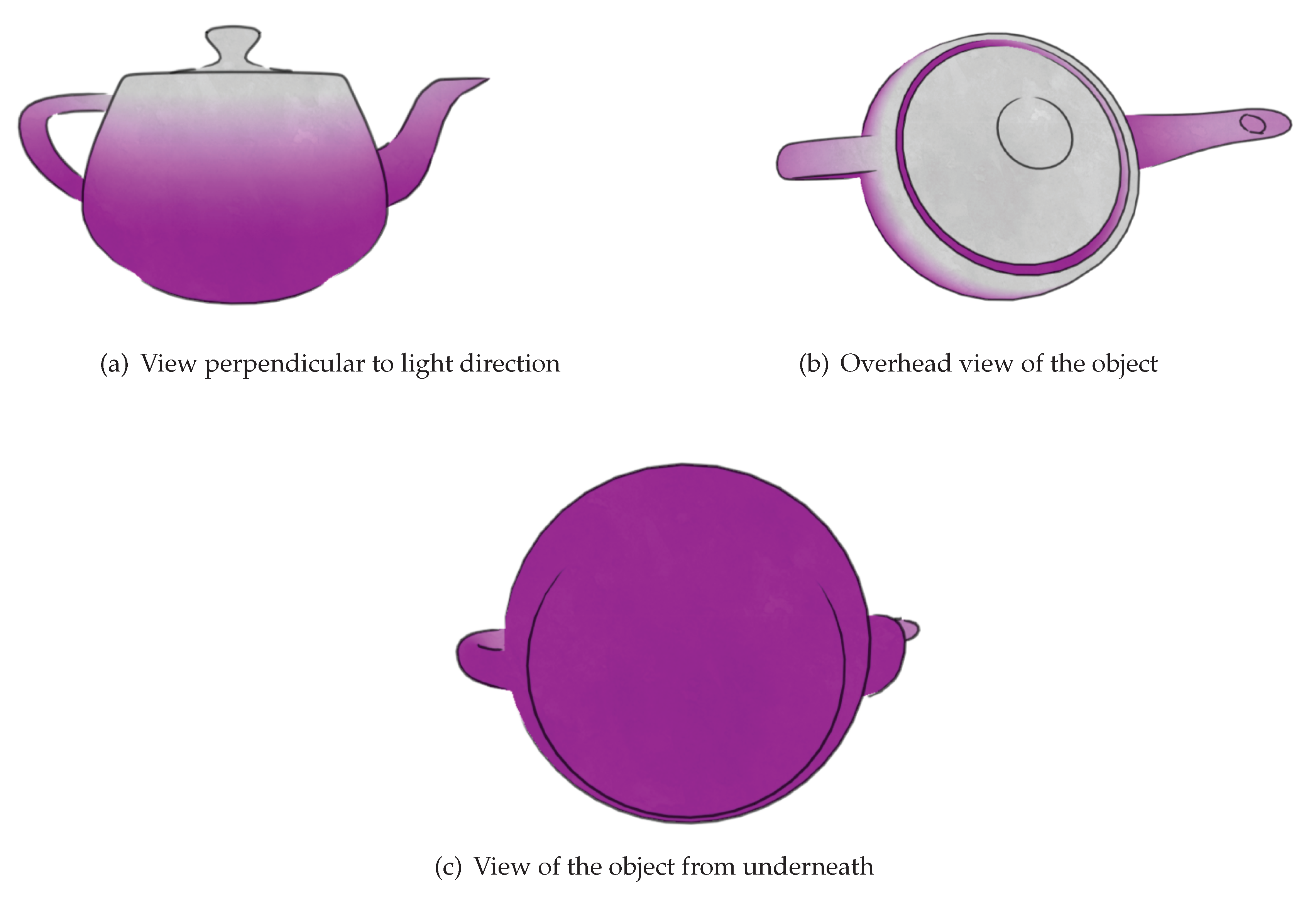
Similar to the texture algorithms, the first bokashi algorithm renders gradation based on a centre point and scales the gradation with depth to maintain temporal coherence as the object is translated in 3D. Furthermore, the view modifier used moves the point of gradation to make the object appear more or less illuminated based on the view position relative to the light. Figure 18 demonstrates how an object appears more or less illuminated based on the viewing position. If the gradation boundary is still within the object when the view position is close to the light ray to the object and then moves across the light ray, the gradation appears to flip to the other side of the object. However, most of the time the gradation smoothly rotates to indicate the direction of light. For the best results, the view modifier and centre position must be set for each object such that they are fully illuminated or unilluminated when the view vector is almost parallel to the light ray to avoid instant flipping of gradation. The problem could also be avoided by only using this algorithm when it is known that the view will not cross or rarely cross the light ray.
A limitation of this algorithm is that the gradation is always linear along a straight line and more complex gradations such as following a curved shape can- not be created. This was by design to mimic the imprecise nature of bokashi but also means that the shape of gradation cannot represent inconsistencies in the printing process. This also means that the algorithms cannot accurately represent multiple light sources as the gradation is only in one direction. Furthermore, the effect created with the same parameters at different resolutions varies as the algorithm is based on screen space operations and parameters based on pixel count. This can be impractical for use with an application targeted for use with multiple resolutions.
3.3.4. Bokashi Algorithm 2
Unlike most of the previous algorithms discussed, this algorithm is not primarily based off 2D calculations in screen space and therefore is not closely bound to the resolution of the image. It does not depend on the viewing position or angle either so is consistent as the view moves about the scene. Instead, all the normals and light vector to use are calculated in world space. This means that like the traditional shading techniques it is based on, it exhibits excellent temporal coherence. This makes this algorithm very practical for use in most 3D scenes which would otherwise use a more standard shading strategy. Furthermore, this rendering strategy works well with multiple light sources so can scale up easily to more complicated scenes while still creating gradation effects that approximate the shape of the object. Figure 19 shows how an object is shaded with this algorithm as the view position changes, a smooth gradation is created which only very approximately follows the shape of the object like in ukiyo-e prints. As this algorithm does still approximate the 3D shape of an object it might appear less like a flat print compared to the first bokashi algorithm. Therefore, which bokashi algorithm is best for a scenario depends on if temporal coherence or a flat, print like appearance is more important.
4. Conclusions and Future Work
In this paper we introduced what to the best of our knowledge are the first algorithms for rendering of 3D objects in ukiyo-e style, suitable for real-time manipulation. We first introduced line rendering algorithms aimed at mimicking the artistic strokes of ukiyo-e prints, with important additional features for the improvement of computational performance and perceptual quality (such as line linking as a means of tracing the shape of objects and maintaining temporal coherence). Next, we proposed colour rendering algorithms which employ a number of strategies for simulating the effects created by physical ukiyo-e printing processes. Most importantly in this context, we describe two algorithms for emulating the bokashi effect, suitable to 3D scenes. A rendering environment was implemented to demonstrate the algorithms on a variety of conventional 3D models. We demonstrated that the algorithms can be implemented using an industry standard graphics API (OpenGL) while performing well in real-time.
Our contributions open a breadth of avenues for future work. For example, as regards the use of perspective as a means of conveying artistic impression, our use of conventional perspective projection makes the end renderings most similar to the relatively short lived uki-e movement in which artists used ukiyo-e printing techniques to create prints with a perspective style inspired by western paintings.
Author Contributions
I.B. contributed to the conception of the work, its implementation, and manuscript preparation. O.A. contributed to the conception of the work, its supervision and overall technical direction, and manuscript preparation. All authors have read and agreed to the published version of the manuscript.
Funding
This research received no external funding.
Conflicts of Interest
The authors declare no conflict of interest.
References
- Bresenham, J.E. Algorithm for computer control of a digital plotter. IBM Syst. J. 1965, 4, 25–30. [Google Scholar] [CrossRef]
- Lake, A.; Marshall, C.; Harris, M.; Blackstein, M. Stylized rendering techniques for scalable real-time 3D animation. In Proceedings of the International Symposium on Non-Photorealistic Animation and Rendering, Annecy, France, 5–7 June 2000; pp. 13–20. [Google Scholar]
- Gooch, B.; Sloan, P.P.J.; Gooch, A.; Shirley, P.; Riesenfeld, R. Interactive technical illustration. In Proceedings of the Symposium on Interactive 3D Graphics, Atlanta, GA, USA, 26 April–2 May 1999; pp. 31–38. [Google Scholar]
- Harris, F. Ukiyo-e: The Art of the Japanese Print; Tuttle Publishing: Clarendon, VT, USA, 2012. [Google Scholar]
- Markosian, L.; Kowalski, M.A.; Goldstein, D.; Trychin, S.J.; Hughes, J.F.; Bourdev, L.D. Real-time nonphotorealistic rendering. In Proceedings of the Annual Conference on Computer Graphics and Interactive Techniques, Los Angeles, CA, USA, 3–8 August 1997; pp. 415–420. [Google Scholar]
- Woo, M.; Neider, J.; Davis, T.; Shreiner, D. OpenGL Programming Guide: The Official Guide to Learning OpenGL, Version 1.2; Addison-Wesley Longman Publishing Co., Inc.: Boston, MA, USA, 1999. [Google Scholar]
- Setthawong, P. Potential Z-Fighting Conflict Detection System in 3D Level Design Tools. In Information Science and Applications; Springer: Berlin/Heidelberg, Germany, 2015; pp. 279–285. [Google Scholar]
- Northrup, J.; Markosian, L. Artistic silhouettes: A hybrid approach. In Proceedings of the International Symposium on Non-Photorealistic Animation and Rendering, Annecy, France, 5–7 June 2000; pp. 31–37. [Google Scholar]
- Everitt, C.; Rege, A.; Cebenoyan, C. Hardware shadow mapping. White Paper nVIDIA, 2001; 2. Available online: https://www-inst.cs.berkeley.edu/~cs283/fa10/lectures/shadow_mapping.pdf(accessed on 10 May 2020).
- Gouraud, H. Continuous shading of curved surfaces. IEEE Trans. Comput. 1971, 100, 623–629. [Google Scholar] [CrossRef]
- Phong, B.T. Illumination for computer generated pictures. Commun. ACM 1975, 18, 311–317. [Google Scholar] [CrossRef] [Green Version]
Figure 1.
Seba by Utagawa Hiroshige.
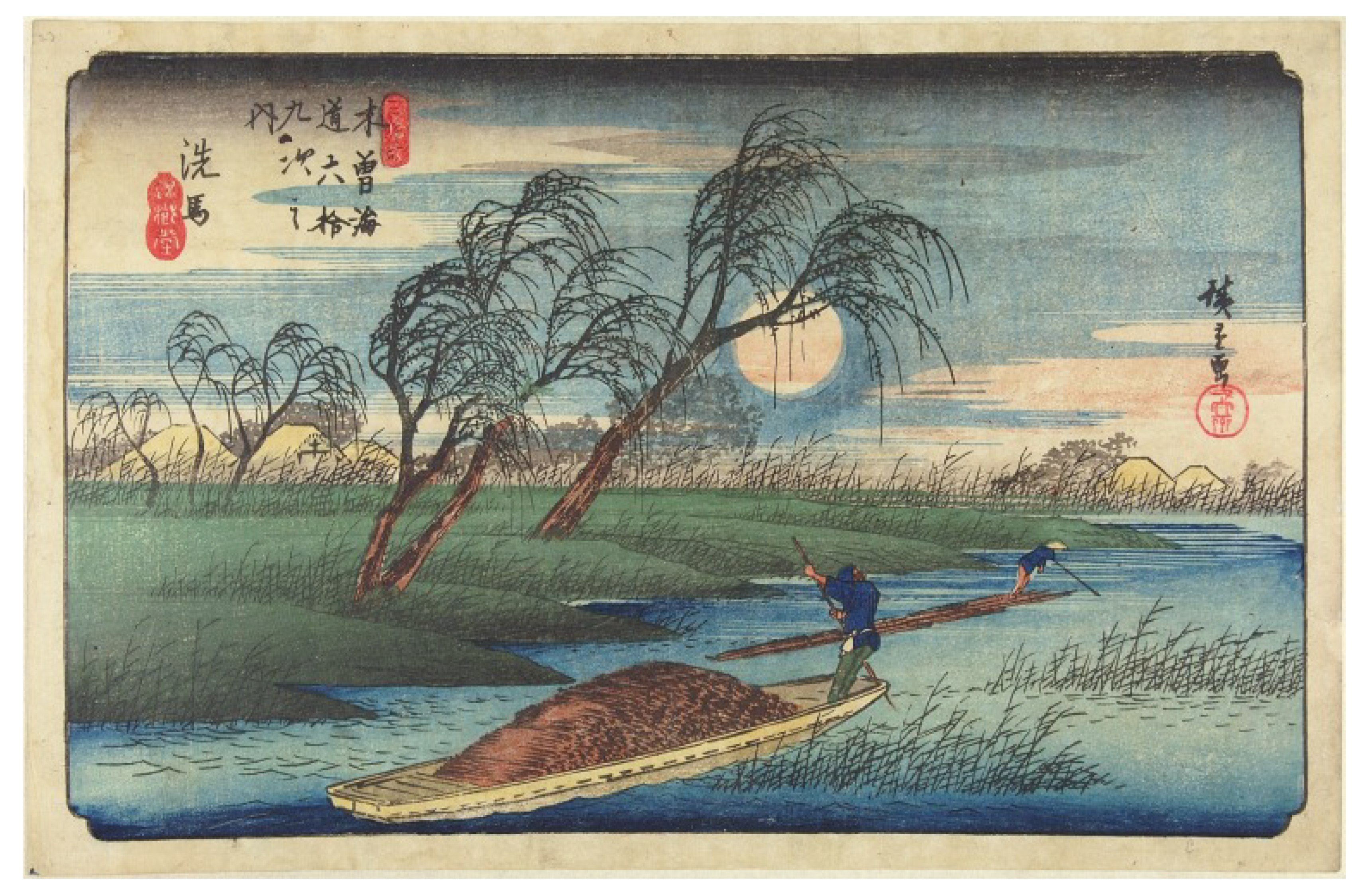
Figure 2.
Initial design for Chunagon Kanesuke by K. Hokusai.
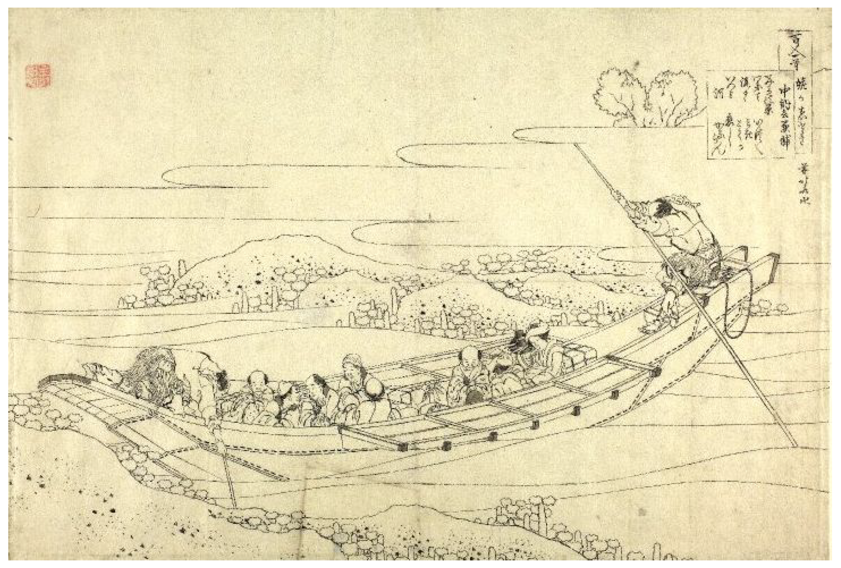
Figure 3.
Our stroke rendering pipeline.

Figure 4.
Synthesised reference image example.

Figure 5.
Examples of different edge segment classification cases.
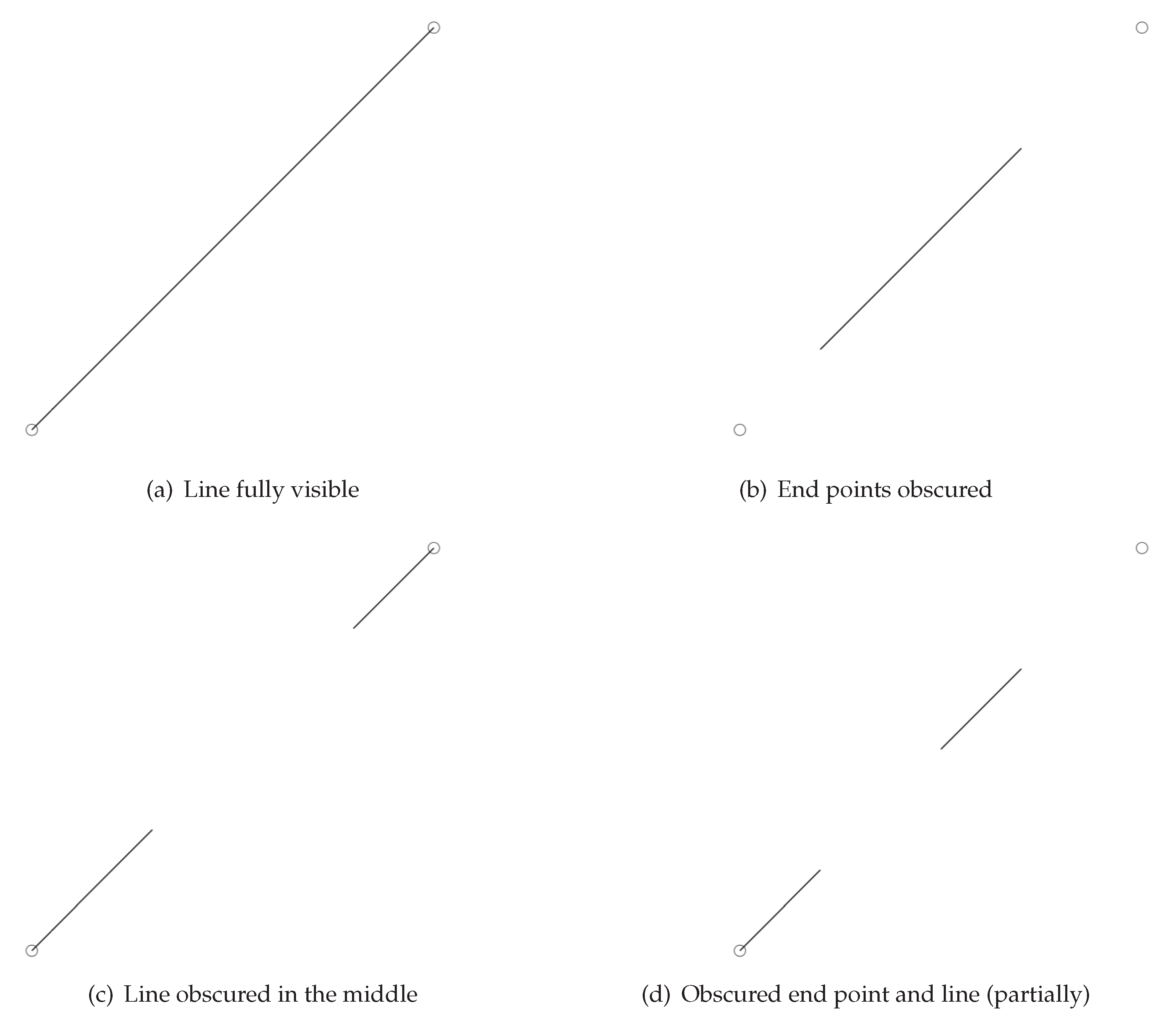
Figure 6.
Example of a typical result produced by our complete line rendering process.

Figure 7.
Example of the application of pseudo-uniform colour with a noise texture.
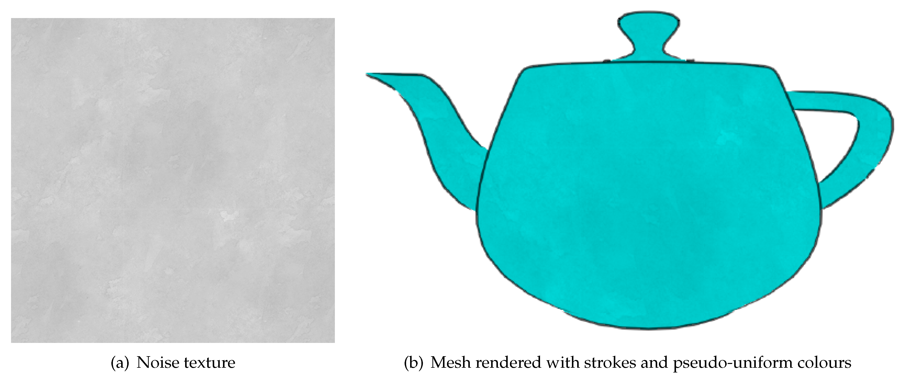
Figure 8.
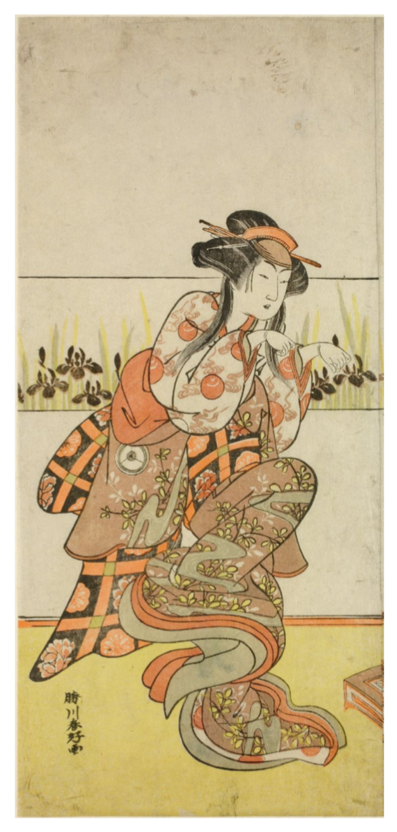
Iwai Hanshiro IV by Katsukawa Shunko.

Figure 9.
An illustration of the application of textured patterns.

Figure 10.
Example of rendering using our first bokashi mimicking algorithm.

Figure 11.
Conceptual illustration of our method for computing sphere normals and the light vector.

Figure 12.
Example of rendering using our second bokashi mimicking algorithm.

Figure 13.
Examples of objects rendered using the proposed framework under different settings.
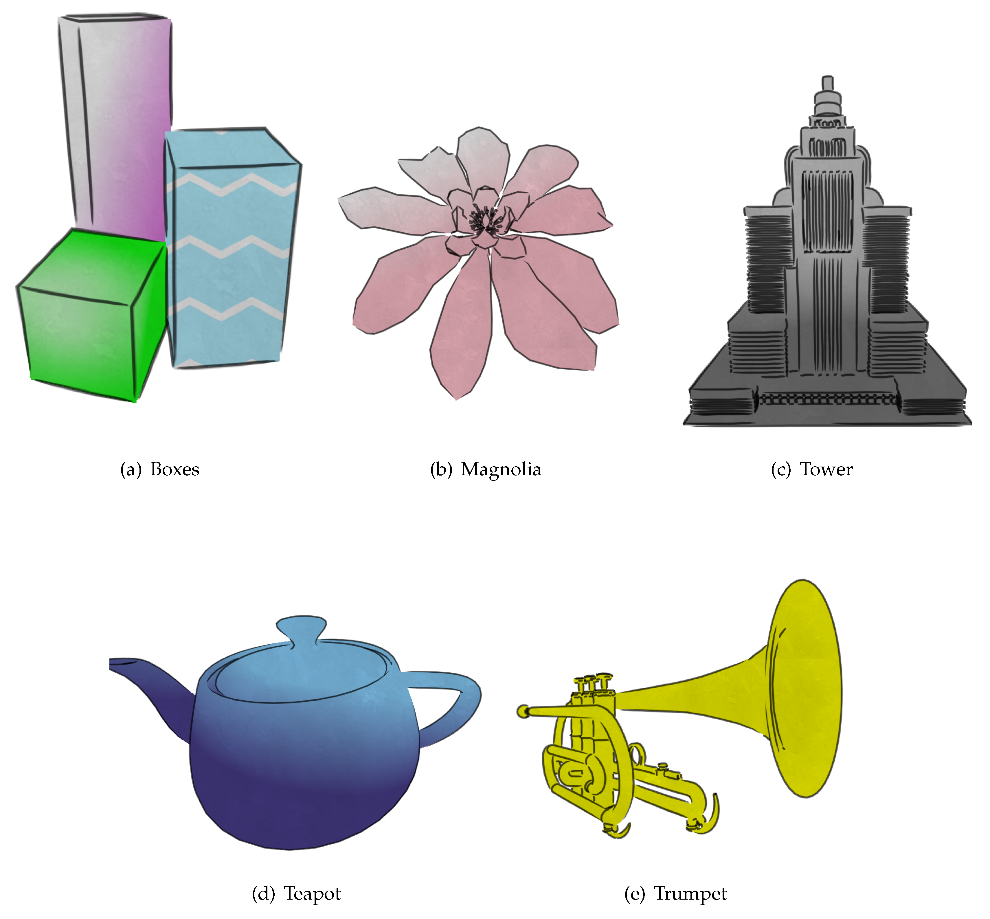
Figure 14.
Summary of frame rate analysis.

Figure 15.
Comparison of rendering a 1080p image with different reference image resolutions.

Figure 16.
Comparison of linear renderings of a distant teapot using different link depths.
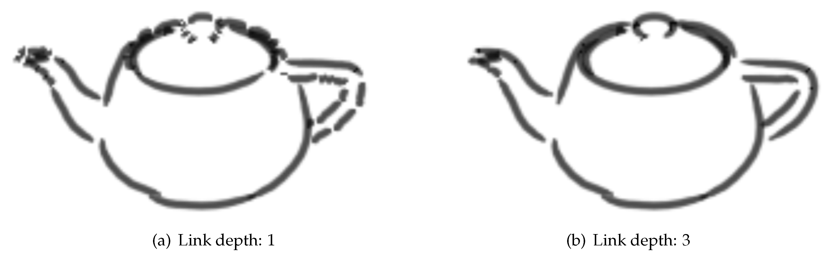
Figure 17.
Example of line rendering errors arising from a high number of allowed misses when tracing edges. Especially observe the region were the teapot handle attaches to the main vessel body.
Figure 17.
Example of line rendering errors arising from a high number of allowed misses when tracing edges. Especially observe the region were the teapot handle attaches to the main vessel body.

Figure 18.
Illustration of colour gradation produced by our first bokashi algorithm, with the object viewed from different directions. Compare with Figure 19.
Figure 18.
Illustration of colour gradation produced by our first bokashi algorithm, with the object viewed from different directions. Compare with Figure 19.
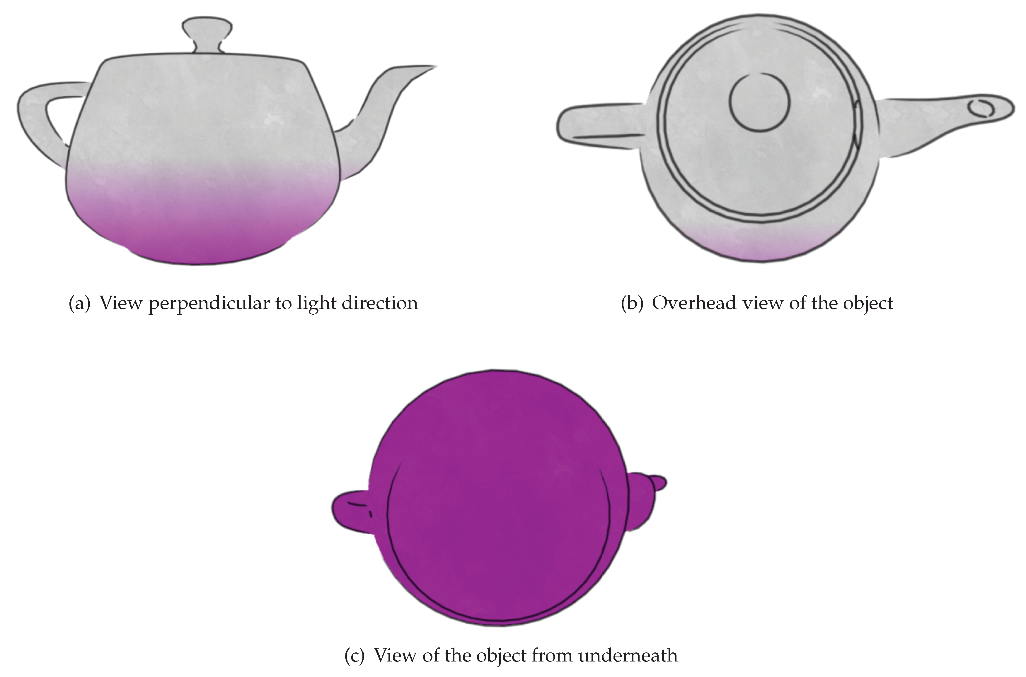
Figure 19.
Illustration of colour gradation produced by our second bokashi algorithm, with the object viewed from different directions. Compare with Figure 18.
Figure 19.
Illustration of colour gradation produced by our second bokashi algorithm, with the object viewed from different directions. Compare with Figure 18.


Table 1.
Polygonal/geometric complexity of rendered object examples.
| Scene | Boxes | Magnolia | Tower | Teapot | Trumpet |
|---|---|---|---|---|---|
| Polygon count | 36 | 1372 | 3676 | 6320 | 23,255 |
© 2020 by the authors. Licensee MDPI, Basel, Switzerland. This article is an open access article distributed under the terms and conditions of the Creative Commons Attribution (CC BY) license (http://creativecommons.org/licenses/by/4.0/).
Share and Cite
MDPI and ACS Style
Brown, I.; Arandjelović, O. Making Japenese Ukiyo-e Art 3D in Real-Time. Sci 2020, 2, 32. https://doi.org/10.3390/sci2020032
AMA Style
Brown I, Arandjelović O. Making Japenese Ukiyo-e Art 3D in Real-Time. Sci. 2020; 2(2):32. https://doi.org/10.3390/sci2020032
Chicago/Turabian StyleBrown, Innes, and Ognjen Arandjelović. 2020. "Making Japenese Ukiyo-e Art 3D in Real-Time" Sci 2, no. 2: 32. https://doi.org/10.3390/sci2020032