Sustainable Design of Pavements: Predicting Pavement Service Life

Abstract

Pavement service life is an important factor that affects both the whole life cost and carbon footprint of a pavement. The service life of a pavement is affected by several different parameters which can be broadly classified into climate conditions, binder and mixture properties, pavement design, workmanship, and maintenance strategies. The current practice for determining service life of pavements involves the use of pavement design tools, which are used while constructing a new pavement or performing a reconstruction/resurfacing or pavement maintenance. In addition, field measurements using ground penetration radar, falling weight deflectometer, traffic speed deflectometer, and other techniques are also used to assess the condition of an existing pavement. The information from these measurements is then combined with pavement design software to predict potential pavement service life. The accuracy of the predicted pavement service life is affected by the associated uncertainties in the parameters that affect pavement life. The following paper presents various approaches that could be potentially used to determine the associated uncertainties in the estimation of pavement service life. The various uncertainty quantification techniques have been applied to a specific design, and the outcomes are discussed in this paper. The Monte Carlo simulation method, a system-level uncertainty quantification technique, can estimate a probabilistic pavement service life. The other uncertainty quantification schemes are software specific and provide probabilistic life factors by assumed statistical distributions. Hence, the Monte Carlo simulation technique could be one potential method that can be used for estimating a generalized pavement service utilizing predictions from various design software.

1. Introduction

The purpose of this paper is to propose a framework for estimating service life of a pavement. The service life of a pavement is a key input for developing LCA models for pavements. The proposed framework has been applied to a standard case wherein a penetration grade binder has been compared to a polymer modified bitumen. This approach can then be applied to various other binder materials and pavement designs, with the aim of understanding sustainability benefits associated with a specific approach.

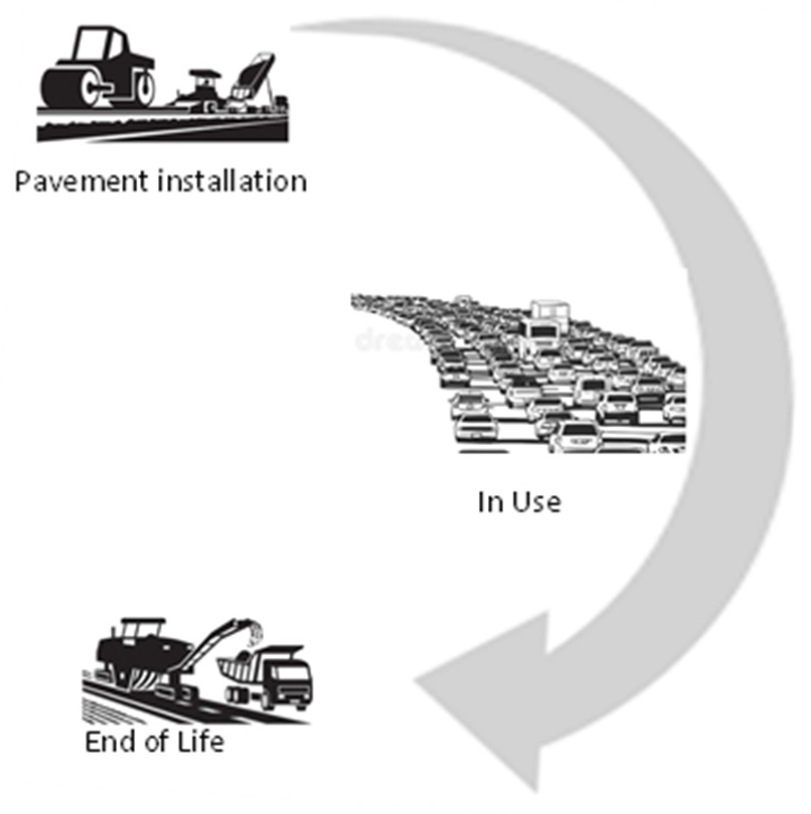
The life cycle of a pavement can be considered as three stages, as described in Figure 1. The whole life energy use and emissions associated with an asphalt pavement is significantly influenced by the service life of the pavement. Pavement construction results in emissions primarily associated with use of materials and energy arising from the extraction of raw materials, making asphalt, transport, and other supply chain-related emissions. Once the pavement is laid, there are emissions associated with periodic maintenance of the pavement and, finally, at the end of the pavement service life, the pavement is removed and then typically reused as recycled asphalt pavement (RAP). It is important to understand the service life of a pavement since that determines the frequency and type of maintenance required; hence, the overall emissions associated with a pavement in a cradle-to-grave, or cradle-to-cradle, approach for life cycle assessments. The design of pavements with an increased service life is one of the key levers from a sustainability perspective and also aligns with the sustainable development goals proposed by the United Nations [1], in particular goals 9 (Industry, innovation and infrastructure), 12 (Responsible consumption and production), and 13 (Climate action), as well as long service life being a key pillar of circular economy thinking and improving resource and materials efficiency by using less materials over a period of time to perform the same function.

The service life of a pavement is affected by various factors such as the design of the pavement, climate conditions, type of binders and asphalt mixtures used, traffic and traffic growth rates, workmanship, and applied loads [2]. There are general design guidelines that are prescribed by various highway agencies in Europe that guide the design of pavements considering these factors [3]. Hence, pavement design tools can then help in determining specific pavement thickness aligning with such specifications. One of the primary ways in which pavement life is determined is supported by measurements of the rutting and fatigue behavior of asphalt mixtures in the laboratory [4]. A further approach that has been adopted is to test cores from the field and fine tune pavement failure models (specifically, rutting and fatigue models) to estimate service life of pavements [5,6].

1.1. Approach to Pavement Design and Quantification of Uncertainty

The current industrial practice for pavement design is to use pavement design software, and there are several different design tools that are currently being used in the market, as shown in

Table 1. Various design tools used for predicting pavement service life.

Software Name	Strain Estimation	Mathematical Procedure	Performance Prediction
BISAR/BANDS	Elastic layered theory	Finite differences	Empirical models laboratory based
AASHTOWARE		Mechanistic empirical pavement design	Field tested empirical models
KENPAVE/KENLAYER		Mechanistic empirical pavement design	Empirical models that account for viscoelasticity
PAVXPRESS		Mechanistic empirical pavement design	Empirical models
CIRCLY		Multi-layer linear elastic theory
IIT PAVE		Mechanistic empirical pavement design
FARFIELD		3D finite element method
EVERSTRESS FE		3D finite element method

.

Most of these tools are mechanistic–empirical design tools where the stress and strain distribution in a pavement is determined by the elastic layer theory and the strain response is then further converted into pavement performance by empirical models. In addition, there are specific empirical models that are used for thermal cracking-type failure and also to determine the elastic modulus of the pavement at different temperatures. The measured dynamic modulus of an asphalt specimen is used as an input for these design tools. The preferred approach today for pavement design is to use a 2D finite element approach for strain prediction and use empirical models for pavement performance. Improving the accuracy of predicted strain, however, generally does not result in improved life prediction as discussed below.

The equation for fatigue (for example in the AASHTOware tool) is as follows

$$\mathrm{N}\mathrm{f}=0.00432\ast \mathrm{C}\ast \mathrm{B}\mathrm{f}1\mathrm{k}1\ast {\left({\displaystyle \frac{1}{\mathsf{\epsilon }}}\right)}^{\mathrm{k}2\mathsf{\beta }\mathrm{f}2}{\left({\displaystyle \frac{1}{\mathrm{E}}}\right)}^{\mathrm{k}3\mathsf{\beta }\mathrm{f}3}$$

(1)

If a partial differential of this equation with respect to strain is performed, then the equation will be as below.

$${\displaystyle \frac{\partial \mathrm{N}\mathrm{f}}{\partial \mathsf{\epsilon }}}=\mathrm{k}2\mathsf{\beta }\mathrm{f}2({\displaystyle \frac{1}{\mathsf{\epsilon }2}})$$

(2)

Nf—number of cycles, E—bulk modulus of the specimen (MPa) C, $\mathrm{k}2\mathsf{\beta }\mathrm{f}2$, $\mathrm{k}3\mathsf{\beta }\mathrm{f}3$—constants, ε—strain in the specimen.

A similar type of correlation, as given in Equation (1), will also apply to the pavement modulus. The results of a sensitivity analysis of equation 1 using partial differential method, indicates that the predicted life is more sensitive to fitting parameters rather than to strain and modulus (see

Table 2. Model sensitivity of AASHTOware fatigue models to various parameters.

Parameter	Sensitivity of the Model (%)
Incremental change in fitting parameters (10%)	22
Incremental change in strain levels (10%)	17
Incremental change in modulus (10%)	17
Incremental change in number of cycles	6

). Since the model is multiplicative in nature, the overall change in the predicted number of cycles for a 10% incremental change in strain and modulus is only 6%. This indicates that improving strain prediction accuracy may not result in an increase in the accuracy of predicted pavement life. It can also be seen in Table 2 that although the model is more sensitive to constants, the degree of change is of the same order. This is achieved since the model has been tuned to field data; laboratory-based models may have a much higher dependency on fitting parameters. Even in the case of field models, the accuracy of the prediction when compared to observations on the field is limited (between 50% and 70%) and also has limited sensitivity, as indicated in the Mechanistic Empirical Pavement Design Guide (MEPDG), published in 2008.

In summary, predicted pavement service life is affected by many factors and, hence, is prone to inaccuracies such as the following.

(1)

The reliability of the empirical models used for predicting pavement life depends on the nature and the quality of data used for tuning model coefficients. Empirical models that are tuned using data from the testing of field cores result in a prediction of pavement life which is lower than what is observed in the laboratory. AASHTOware uses data generated by testing cores from the field for tuning model coefficients.

(2)

The assumption of the elastic layered theory for stress dissipation across the layers results in variations in the predicted strains [7]

(3)

Performance assessment of field cores requires the use of a falling weight deflectometer (FWD), traffic speed deflectometer (TSD)-type data which, when compared to laboratory techniques to determine asphalt mixture modulus, have very different accuracy levels resulting in differences in predicted pavement life.

(4)

Growth rate assumptions for traffic and loads, plus the uncertainty in accounting for environmental events like high/low temperatures, amount of rainfall etc., may also result in inaccuracies in the predicted pavement life.

As indicated above, the pavement life determined from laboratory data and as observed in the field can differ significantly due to many reasons; hence, it is it is advisable to develop a method for uncertainty quantification associated with pavement life prediction so that a probabilistic pavement service life can then be used in life cycle estimates for pavements.

1.2. Proposed Methods for Uncertainty Quantification

One of the ways that uncertainty quantification has been proposed for pavements is to use a statistical distribution for service life prediction; in this case, a Poisson’s distribution [7]. Poisson’s distribution is a common method to estimate probability of occurrence of an event basis of a set of discreet independent occurrences or data points. The mathematical form of Poisson’s distribution is

$$\mathrm{P}(\mathrm{k}){\displaystyle \frac{{\mathsf{\alpha }}^{\mathrm{k}}{\mathrm{e}}^{-\mathsf{\alpha }}}{\mathrm{k}!}}$$

(3)

α—number of events that have occurred

k—a specific event

P(k)—the probability of occurrence of the k th event.

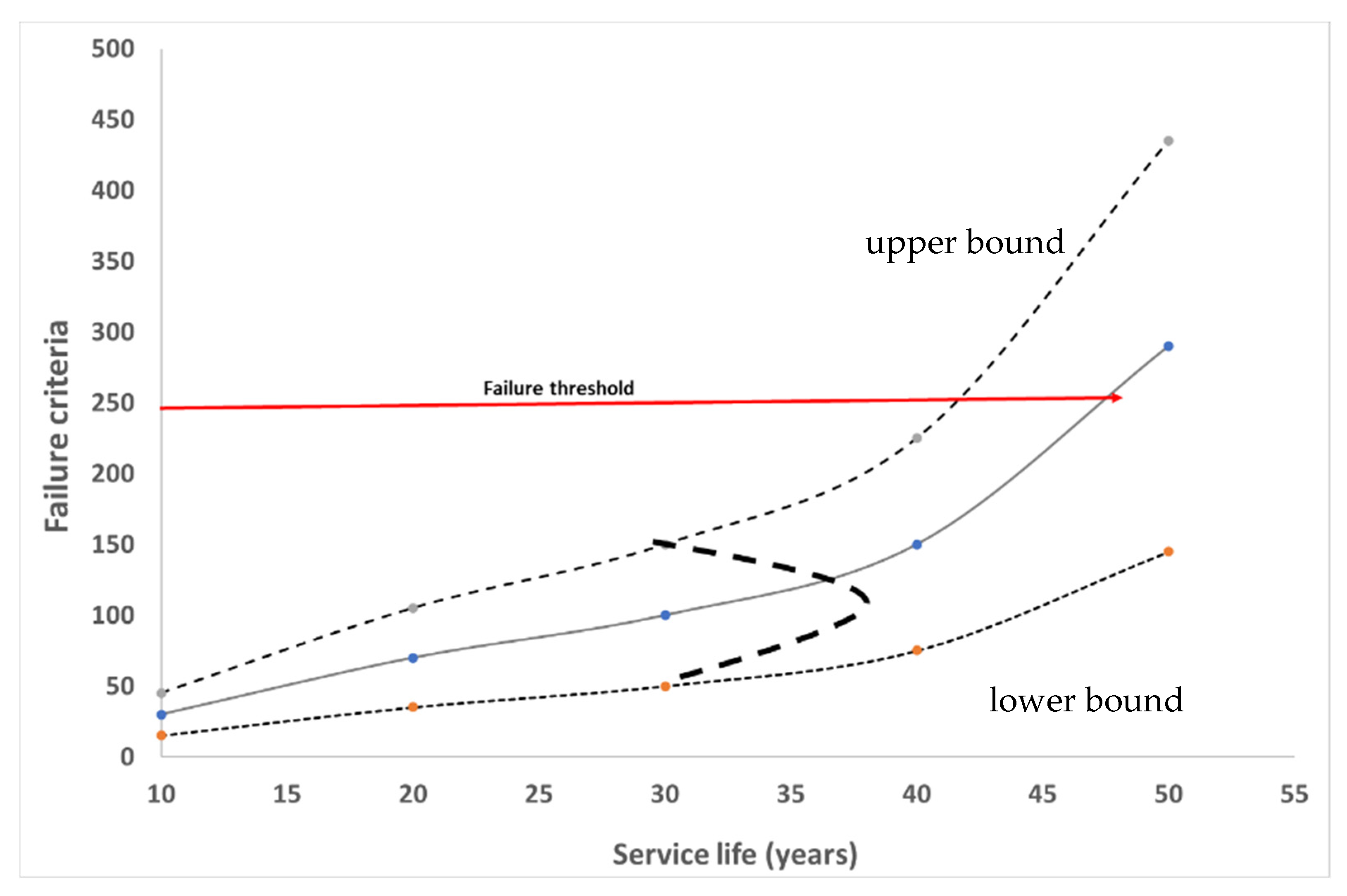
This procedure involves estimation of the pavement performance parameters at three different time points. Once this is completed, the performance parameters are then fitted to the Poisson’s distribution (See Figure 2). The use of Poisson’s distribution then enables the determination of the standard deviation associated with a specific performance criterion. This also enables the determination of a probabilistic pavement service life (at 90% confidence level) for a specific pavement design methodology. This approach can be applied to any pavement design tool where the standard deviations associated with a performance prediction using an empirical model is not established. The reliability of a specific pavement performance model does not account for the accuracy of the model. A very high model reliability is not indicative of high accuracy, specifically where accuracy is defined by how close the predicted numbers are with respect to field observations; hence, a statistical uncertainty quantification technique is required and applied [7]. In this study, the following approach has been used with the AASHTOware design tool.

Since a number of different pavement design tools are used for making service life predictions, a system-level uncertainty quantification technique, such as Monte Carlo simulation, has also been used [8].

The Monte Carlo simulation technique has been widely used in the area of pavement design. The primary application has been in the life cycle cost estimation analysis for pavements wherein the pavement life is already known [9]. Several studies have applied the Monte Carlo simulation technique to determine the impact of variation in factors like traffic and frequency of loading, on pavement thickness from a perpetual pavement design perspective [10,11,12,13].

The current study applies the Monte Carlo simulation technique for estimating a reference pavement life, wherein the pavement life is determined using various pavement design tool. Since the pavement life is estimated using three different software systems which utilize different types of empirical performance models, this method of uncertainty quantification is considered to be a system-level approach.

The Monte Carlo simulation technique assumes discrete probabilities of occurrences of events and, hence, is not biased by assumptions of specific probability density functions. There are several factors in the pavement design process which can be considered as random in nature such as workmanship or the occurrence of extreme weather events. Completely random events cannot be modelled by continuous probability density functions and, hence, the Monte Carlo simulation technique becomes useful for making probabilistic estimates of service lives. In the case of the Monte Carlo technique, discrete probabilities of occurrence are converted to cumulative probability distributions, which are then evaluated with various random numbers generated between chosen thresholds [9]. This scenario is described in Figure 3.

Three different pavement design tools are considered in this paper. These three tools are representative of the approaches that are generally used in practice for making service life estimates (as shown in Table 1). These also represent three different scenarios with regard to prediction of pavement service life as shown in

Table 3. Design tools used in this study for estimating pavement service life.

Design Tool	Comments	Life Prediction Scenario
AASHTOware	Validated with field data	Pessimistic
Shell pavement design method (SPDM)	Based on laboratory data	Optimistic
Kenpave	Accounts for viscoelasticity of asphalt pavements and is partially laboratory data based	Neutral

.

Empirical models used for prediction of pavement life in AASHTOware are validated using field data. In addition, since the models are empirical and tuning of the models is carried out using regression techniques, the models themselves have a specific accuracy (with an R² between 70% and 90%) [5,6,7]. Hence, there is further reduction of the predicted service life beyond what is observed in practice. From a scenario analysis perspective, this has been considered to be pessimistic.

The shell pavement design method (SPDM) is based on laboratory data wherein all parameters affecting pavement performance can be controlled. Pavement service lives predicted using laboratory data are higher than observed in the field; hence, prediction of service life using the SPDM method has been considered to be optimistic.

There are several studies that have indicated that when SPDM is used, the thickness of a pavement for a given service life is overestimated; hence, for a specified thickness the fatigue life will be a overestimated [14,15,16]. The SPDM method is based on the initial binder properties of the material only since the models are not tuned to field data; hence, does not account for ageing of the binder, resulting in overestimation of pavement life [14,16].

The equation used for determining pavement life using SPDM is as below.

$$\mathrm{N}=4.91\times {10}^{-13}{(0.86\mathrm{V}\mathrm{b}+1.08)}^5{({\displaystyle \frac{1}{\mathsf{\epsilon }}})}^5{\left({\displaystyle \frac{1}{\mathrm{S}\mathrm{m}\mathrm{i}\mathrm{x}}}\right)}^{1.8}$$

(4)

$$\mathrm{N}=\mathrm{k}{\mathsf{\epsilon }}^{\mathrm{n}}$$

(5)

N—number of load cycles to failure

Vb—volume of asphalt in the mixture (%) (13% assumed for the case discussed in the paper)

ε—maximum tensile asphalt concrete strain (micrometer/micrometer) (250 microstrains)

S_mix—dynamic modulus of the asphalt mixture (MPa).

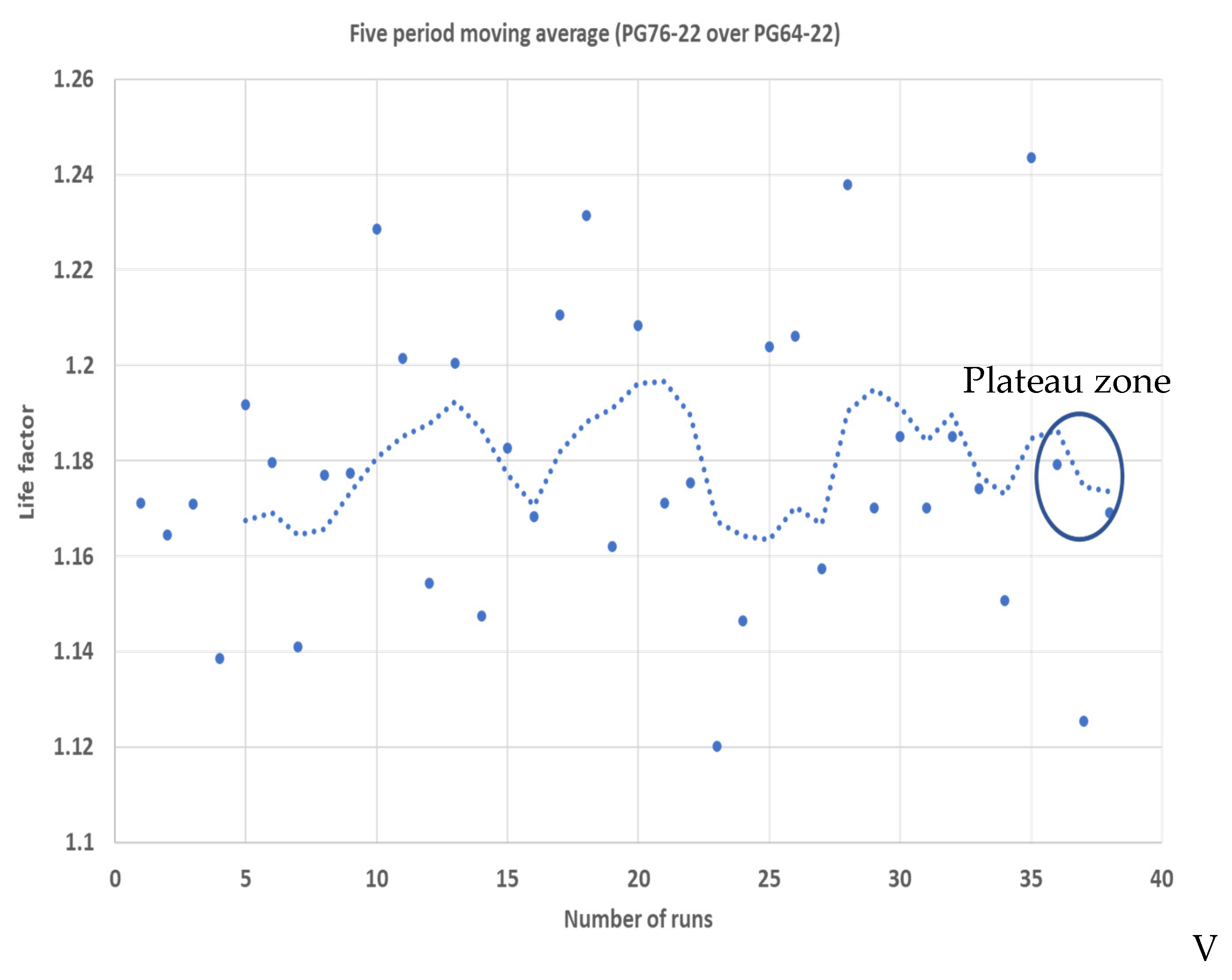
In addition to the above model, the fatigue life of an asphalt specimen was determined as as per the pavement design and gradation in

Table 4. Base boundary conditions used for simulating pavement life using AASHTOware.

Layer Details	Comments
Surface course (thickness)	50 mm with a PG76-22
Binder course (thickness)	130 mm with a PG64-22
Subbase (thickness)	180 mm with a resilient modulus of 80 MPa
Subgrade (thickness)	150 mm gravel subgrade
Air void content (%)	6%
Binder content (w/w)	4.80%
Mean annual air temperature (Celsius)	22.9
Mean annual precipitation (mm)	1106
Freezing index (number of subzero days)	3
Average annual number of freeze thaw cycles	1
Number of wet days	210
Highest air temperature (Celsius)	37

and

Table 5. Aggregate gradation used in this study.

Sieves Size SI (mm)	Gradation, Percent Passing
25	100
19	99
12.5	70
9.5	64
4.75	36
2.36	24
1.18	19
0.6	16
0.3	11
0.15	8
0.075	5

respectively, and the parameters k and n were determined for both PG64-22 and PG76-22. A design ESAL of 1000/day was used in the SPDM model. The Kenpave simulation was performed using the same inputs as used in the SPDM with a difference that a viscoelastic interface was selected while calculating the strain levels in the specimen.

Kenpave is a design tool that is partially based on laboratory data and partially based on published field testing data since it uses generic equations proposed by the Asphalt Institute, which are field tested but not calibrated to the extend as performed for AASHTOware. In addition, Kenpave assumes a viscoelastic interface between pavement layers and, hence, accounts for field behavior and simulates the rheological nature of the asphalt layers more closely; hence, it is considered to be a neutral scenario in terms of service life prediction [17].

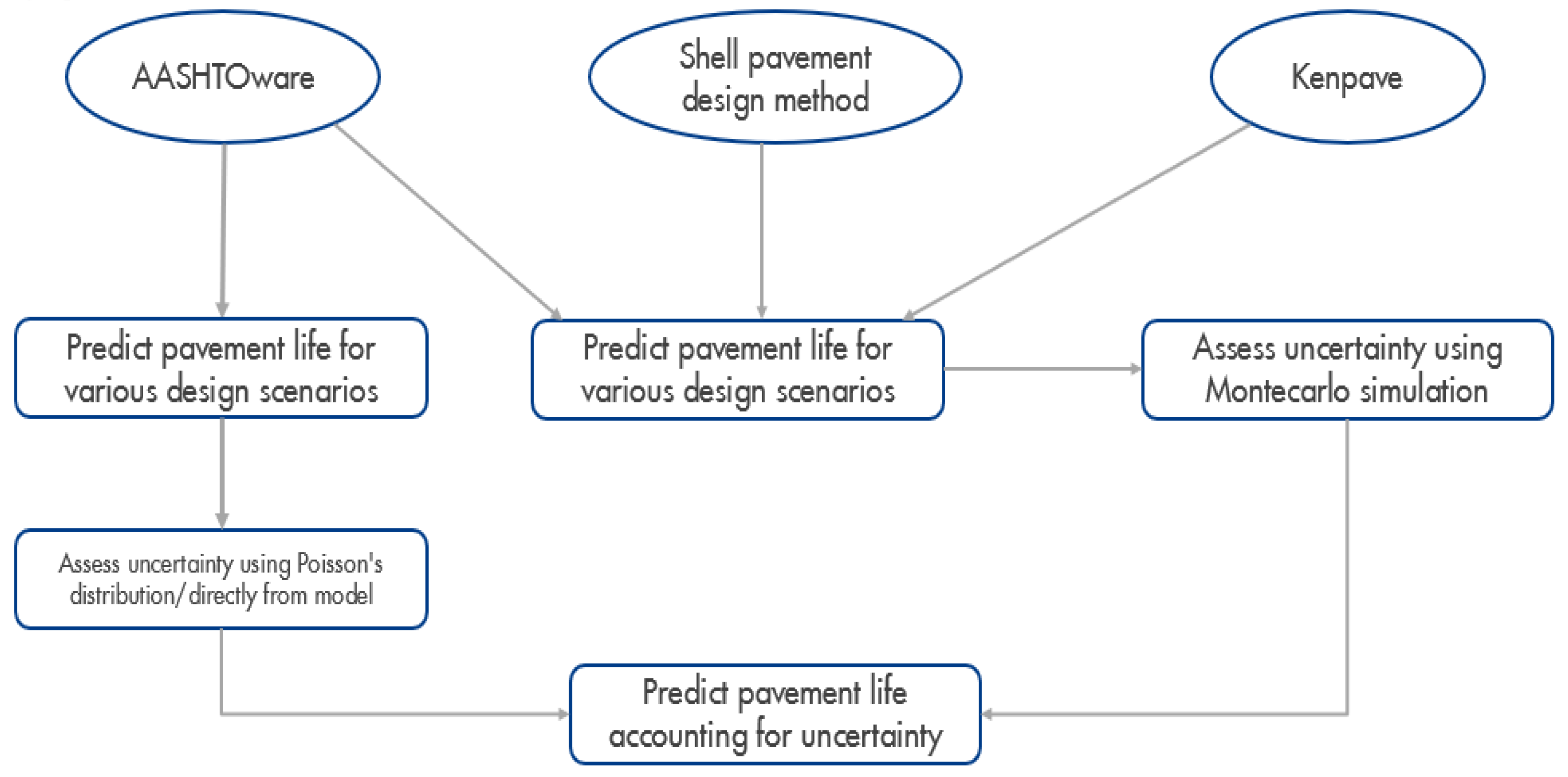
Some of the empirical performance models used in the AASHTOware approach have reported standard deviations, which can then be used for estimating uncertainty of predictions for point estimates. Hence, this method of uncertainty quantification can also be used for making probabilistic estimates, but this information is limited to very few tools and also to very few types of performance parameters; hence, is not a procedure that can always be used for quantifying uncertainty. In addition, even if this information is available for all the design tools and performance parameters, each predicted probabilistic service life will then require application of Monte Carlo simulations to estimate system-level uncertainties and also a unique pavement service life for a specific design. Hence, in this paper, only two different techniques have been evaluated. The methodology adopted in prediction of pavement service life accounting for uncertainty is shown in Figure 4.

2. Results and Discussions

For a test case using the following three methods of uncertainty, quantification of a pavement design is investigated, which considers a PG76-22-based surface course (Styrene-Butadiene-Styrene modified bitumen) over a binder course made using PG64-22 (unmodified bitumen). The base case used in this scenario has both layers made using unmodified PG64-22-based mixtures and is shown in Figure 5. The binder content and air void contents of the two cases are identical. In the case of AASHTOware, a level 3 input for binder properties and asphalt properties has been applied.

The pavement in this case is a four-layer standard construction with a surface course, binder course, subbase, and subgrade layer. A perfect bonding between the asphalt layers has been assumed for estimating the pavement life and a dense mixture gradation as per Superpave MS2-1 has been used, as shown in Table 5. The thickness and various layer properties are summarized in Table 4. The design presented in this paper considers an average quality of subbase and subgrade. This design has been chosen so that the pavement life is dependent on the properties of the asphalt layers. The estimated pavement life using the three design tools is shown in

Table 6. Base boundary conditions used for simulating pavement life using SPDM.

Layer Details	Comments
Surface course (thickness)	50 mm with a PG76-22
Binder course (thickness)	130 mm with a PG64-22
Subbase (thickness)	180 mm with a resilient modulus of 80 MPa
Subgrade (thickness)	150 mm gravel subgrade
Air void content (%)	6%
Binder content (w/w)	4.80%
Mean annual air temperature (Celsius)	22.9
ITSM (MPa) at 20 °C for PG76-22	2852
ITSM (MPa) at 20 °C for PG64-22	3210
Penetration (PG76-22) (dmm)	45
Softening point (°C) (dmm)	83.5
Penetration (PG64-22) (dmm)	63
Softening point (°C) (dmm)	48.6
Poisson’s ratio	0.35
Log k (PG 64-22)	32
Power index (PG64-22)	−3.6
Log k (PG 76-22)	35.5
Power index (PG 76-22)	−2.2
Strain level (micrometer)	250
ESAL/day	1000

. A similar four-layer pavement design has been used while determining pavement life using SPDM and Kenpave. The input parameters used with SPDM is summarized in Table 6.

Kenpave uses the same information as for SPDM in terms of layer thickness, the difference being the pavement performance equations used are as developed by the Asphalt Institute [18]. Also in this simulation, a viscoelastic interface has been chosen in the layer properties, specifically when a PG76-22 binder is used. The creep compliance data that has been used to model viscoelastic materials using Kenpave is shown in

Table 7. Creep compliance data for Kenpave where viscoelastic option is chosen.

Loading Time (Seconds)	−20 °C (1/GPa)	−10 °C (1/GPa)	0 °C (1/GPa)
1	0.0679	0.1	0.145
2	0.073	0.116	0.171
5	0.0824	0.14	0.226
10	0.089	0.161	0.282
20	0.097	0.186	0.352
50	0.109	0.224	0.472
100	0.118	0.263	0.589

.

The predicted pavement life using the different design tools shows a very big range, with service life varying between 20 and 32 years for the base case and between 40 and 60 years for the case of the PG76-22 surface course, as shown in

Table 8. Predicted pavement life with the three different design tools.

	Pavement Life (Years)
Design tool used	PG 64-22 binder course and PG 64-22 surface course	PG 76-22 surface course over PG 64-22
AASHTOware [19]	20	40
SPDM [20]	32	60
KENPAVE [21]	24	51

. As expected, there is a wide variation in the predicted service life of a pavement, the application of an uncertainty quantification technique can then enable estimating an average pavement service life for the presented case. The predicted life in this case is a deterministic estimate of a pavement life.

Table 9. Application of Poisson’s distribution for pavement life prediction.

Pavement Life (Years)	Pavement Type	Description	Standard Deviation
	Overlay (50 mm)	PG6422 over PG6422
10	127.4	AC thermal cracking (m/km)
20	295.3
5	91.8
9	122.5	188.5	66
		PG7622 over PG6422
20	133.9	AC thermal cracking (m/km)
30	225.8
10	88.1
12.5	97.3	188.30	91.0
Normalized life factor with reference to base case		1.4

summarizes the outcomes for the two cases where the uncertainty quantification is completed by applying Poisson’s distribution. The application of Poisson’s distribution is made by estimating pavement performance parameters at three different service lifes and two different reliability levels (50% and 90%). It is then assumed that the reliability levels indicate a probability of 50% and 90% on the Poisson’s distribution. The primary mechanism of pavement failure in this case is thermal cracking of the asphalt layer and has a set design cutoff criteria of 189 m/km. The thermal cracking parameter is then fitted to a Poisson’s distribution to estimate a pavement life at 90% reliability level. It can be seen from Table 9 that accounting for uncertainty by the Poisson’s distribution technique results in a pavement life of 9 years for the base case (PG64-22 overlay over a PG64-22 binder course) and a pavement life of 12.5 years for the case of pavement with a PG76-22 surface course overlaid over a PG64-22 binder course. Hence, the life factor with respect to the base case is 1.4. This is obtained by dividing the pavement life for the 2 scenarios (12.5/9).

The estimation of pavement life was also carried out using the Monte Carlo simulation technique utilizing the procedure and the weighting factors described previously in Figure 4. The pavement life was determined for each of the scenarios as per the weighting scheme. Once the life factor was estimated for each scenario, an average life factor was determined. The life factor as per Monte Carlo simulation was determined using a five-period moving average technique. The moving average stabilizes to a plateau as the number of simulations within the prescribed limit increases. The random numbers are generated using a random number generator. The simulation is terminated when the change in the five-period moving average is less than 10% and the service life for the pavement is determined.

The Monte Carlo simulation technique, if required, can be applied to a bigger sample set as well as where the service life of the pavement is estimated using more pavement design tools. The only change in such a scenario would be that the weighting factor schemes would change accordingly to account for higher number of input service life. It can be seen from Figure 6 and Figure 7 that the life factor for the above two cases are 1.17 and 1.30, respectively. The effect of applying the Monte Carlo simulation technique on predicted pavement service life is summarized in Table 8, where it can be seen that without application of uncertainty, the life factor, with respect to the base case, is 2. After application of the Monte Carlo simulation technique, the life factor comes down to a value of 1.5, as shown in Table 10. The life factor calculations are as below.

Base life of the pavement with a PG76-22 binder = 20 years

Life as per Monte Carlo simulation = 1.15 * 20 = 23 years

Incremental life factor if PG76-22 is used in place of PG64-22 = 23/13.2 = 1.5

Figure 6. Monte Carlo simulation results for a PG76-22 overlay on a PG64-22.

Figure 6. Monte Carlo simulation results for a PG76-22 overlay on a PG64-22.

Figure 7. Life factor estimation using Monte Carlo simulation technique.

Figure 7. Life factor estimation using Monte Carlo simulation technique.

Table 10. Life factor estimates using Monte Carlo simulation technique.

AASHTOware	SPDM	KENPAVE	Weighted Life Factor PG6422 over PG6422	Weighted Life Factor PG7622 over PG6422
0.3333	0.3333	0.3333	1.27	1.26
0.5	0.25	0.25	1.20	1.19
0.25	0.25	0.5	1.25	1.26
0.25	0.5	0.25	1.35	1.32
0.75	0.125	0.125	1.10	1.10
0.125	0.75	0.125	1.48	1.41
0.125	0.125	0.75	1.23	1.27
Average factor			1.27	1.26
Base life			10.00	20.00
Estimated life			12.67	25.17
Monte Carlo estimate (50 runs)			1.32	1.15
Estimated life			13.20	23.00
Normalized life factor wrt base case				1.50

Table 10. Life factor estimates using Monte Carlo simulation technique.

AASHTOware	SPDM	KENPAVE	Weighted Life Factor PG6422 over PG6422	Weighted Life Factor PG7622 over PG6422
0.3333	0.3333	0.3333	1.27	1.26
0.5	0.25	0.25	1.20	1.19
0.25	0.25	0.5	1.25	1.26
0.25	0.5	0.25	1.35	1.32
0.75	0.125	0.125	1.10	1.10
0.125	0.75	0.125	1.48	1.41
0.125	0.125	0.75	1.23	1.27
Average factor			1.27	1.26
Base life			10.00	20.00
Estimated life			12.67	25.17
Monte Carlo estimate (50 runs)			1.32	1.15
Estimated life			13.20	23.00
Normalized life factor wrt base case				1.50

The effect of uncertainty quantification on the service life of a pavement is shown in

Table 11. Summary of life factors determined by the two uncertainty quantification technique.

Description	Incremental Life Factor wrt Base Case (10-Year Design Life)
Monte Carlo approach	5 years
Poisson’s distribution approach	4.5 years
Without uncertainty	12+ years

. The incremental service life of a pavement as compared to the base case is more than 12 years in absence of any uncertainty quantification, and it reduces to 4.5 to 5 years with the uncertainty quantification technique.

The CO₂ eq benefit for using a pavement containing polymer modified bitumen is shown in

Table 12. CO₂ eq benefits of using a polymer modified bitumen.

CO2 Footprint of Unmodified Binder (PG64-22)	132.2	kgCO2eq/t Asphalt
CO2 footprint of PMB (PG76-22)	135.41	kgCO2eq/t asphalt
Emissions per km of road (3.5 m wide) unmodified binder	56	tCO2eq/km
Emissions per km of road (3.5 m wide) PMB	57	tCO2eq/km
Overall pavement service life	100	years
Unmodified binder pavement life (before maintenance) (years)	10	years
PMB-based pavement life (before maintenance) (years)	15	years
No of overlays (unmodified binder)	10	NA
No of overlays (PMB)	7	NA
Avoided emissions	181	tCO2eq/km

. It can be seen from the table that although the initial footprint for a PMB binder is higher than a unmodified binder, since the life of the pavement is higher with a PMB, there is a benefit from an avoided emissions perspective. The emissions associated with the CO₂ eq footprint of binders and asphalt is as per internal reports. A separate paper covering a detailed LCA analysis corroborating the numbers mentioned will be published in due course. This has not been discussed in this paper since the aim of the paper is to propose a method for predicting pavement life.

The numbers mentioned in Table 11 are from cradle-to-pavement laying only.

3. Conclusions

Two different methods of uncertainty quantification for predicting service life of pavements have been described in this paper. As discussed in the paper, there are various reasons that result in uncertainty in estimating the pavement life. The quantification of this uncertainty in predicting service life of pavements is essential to perform whole life cycle cost and carbon assessments on pavements. In addition, the determination of service life of pavements can also help in comparing different binders and/or materials that are used for making asphalt.

Monte Carlo simulation technique is proposed as a method for uncertainty quantification since it is a system-level uncertainty quantification technique. In addition, it can model cases where the input parameters themselves are probabilistic instead of being deterministic. Several different pavement design scenarios like asphalt mixtures which contain recycled asphalt pavement (RAP) for surface and binder courses, use of polymer modified bitumen with different levels of polymer modifications, and the effect of various maintenance strategies on pavement service life can be determined using this technique. This will then help in developing pavement design strategies with an aim of increasing the service life of a pavement. The results in this study indicate that a PG76-22 binder can provide an incremental pavement life of 5 years as compared to a PG64-22 when used in the surface course using a dense mixture design, wherein a PG76-22 type binder is considered to be a polymer modified bitumen and PG64-22 is considered to be an unmodified binder. The cumulative avoided emissions benefit if a PMB-based pavement is used in an overlay scenario over a pavement use life of 100 years is 181 t CO₂eq/km.

References

1. Komen, K. Framework for Green Economy Transition: Towards a Low Carbon, Climate Resilient and Resource Efficient City; City of Tshwane: Tshwane, South Africa, 2013. [Google Scholar]
2. Lavin, P. Asphalt Pavements: A Practical Guide to Design, Production, and Maintenance for Engineers and Architects; Taylor, and Francis: Oxford, NY, USA, 2013. [Google Scholar]
3. Design Manual for Roads and Bridges, CD226: Design for New Pavement Construction; Highways England: Birmingham, UK, 2016.
4. Mogawer, W.; Austerman, A.; Daniel, J.; Zhou, F.; Bennert, T. Evaluation of the effects of hot mix asphalt density on mixture fatigue performance, rutting performance and MEPDG distress predictions. Int. J. Pavement Eng. 2011, 12, 161–175. [Google Scholar] [CrossRef]
5. Gao, Y.; Geng, D.; Huang, X.; Cao, R. Prediction of Remaining Service Life of Asphalt Pavement Using Dissipated Energy Method. J. Transp. Eng. Part B Pavements 2018, 144, 04018011. [Google Scholar] [CrossRef]
6. Billigiri, K.; Said, S. Prediction of remaining fatigue life of flexible pavements using laboratory and field correlations. J. Mater. Civ. Eng. 2015, 27, 04014201. [Google Scholar] [CrossRef]
7. Das, A.; Shukla, P. A revisit to the development of fatigue and rutting equations used for Asphalt pavement design. Int. J. Pavement Eng. 2008, 9, 355–364. [Google Scholar]
8. Sin, G.; Espuna, A. Applications of Monte Carlo Method in Chemical, Biochemical and Environmental Engineering. Front. Energy Res. 2020, 8, 68. [Google Scholar] [CrossRef]
9. Herbold, K. Using Montecarlo simulation for pavement cost analysis. Public Roads 2000, 64, 2–6. [Google Scholar]
10. HazariJafari, H.; Yahia, A.; Amor, B. Assessing the individual and combined effects of uncertainty and variability sources in comparative LCA of pavements. Int. J. Life Cycle Assesment 2018, 23, 1888–1902. [Google Scholar] [CrossRef]
11. Dilip, D.; Ravi, P.; Babu, G.L. System reliability analysis of flexible pavements. J. Transp. Eng. 2013, 139, 1001–1009. [Google Scholar] [CrossRef]
12. Lemer, A.C.; Moavenzadeh, F. Reliability of highway pavements. In Transportation Research Record; Highway Research Board: Washington, DC, USA, 1971. [Google Scholar]
13. Swei, O.; Gregory, J.; Kirchan, R. Probabilistic life cycle costs of pavements: Characterization and application of parameter input variation for scenarios. In Transportation Research Record; Highway Research Board: Washington, DC, USA, 2016. [Google Scholar]
14. Pereira, P.; Pais, J. Main flexible pavement and mix design methods in Europe and challenges for the development of an European method. J. Traffic Transp. Eng. 2017, 4, 316–346. [Google Scholar] [CrossRef]
15. Saleh, M. Calibration and Validation of the Shell Fatigue Model Using AC10 And AC14 Dense Graded Hot Mix Asphalt Fatigue Laboratory Data. Eng. J. 2012, 16, 127–136. [Google Scholar] [CrossRef]
16. Classen, A.; Edwards, J.; Sommer, P. Asphalt pavement design: The Shell method. In Proceedings of the Transportation Research Board International Conference on Structural Design of Asphalt Pavements, Ann Arbor, Michigan, 22–26 August 1977. [Google Scholar]
17. Ahmed, A.; Erlingsson, S. Viscoelastic response modelling of a pavement under moving load. Transp. Res. Procedia 2016, 14, 748–757. [Google Scholar] [CrossRef]
18. MEPDG (Mechanistic Empirical Pavement Design Guide), 3rd ed.; AASHTO: Washington, DC, USA, 2020.
19. AASHToware, Version 2.6. Pavement Design Software. Available online: https://www.aashtoware.org/ (accessed on 3 May 2024).
20. SPDM (Shell Pavement Design Method), Version 2.0. Available online: https://trid.trb.org/View/683379 (accessed on 3 May 2024).
21. Kenpave 1.0. Available online: https://kenpave.software.informer.com/1.0/ (accessed on 3 May 2024).
Figure 1. The pavement life cycle.
Infrastructures 09 00165 g001
Figure 2. Application of Poisson’s distribution to estimate uncertainty in pavement service life.
Infrastructures 09 00165 g002
Figure 3. Monte Carlo simulation technique used for predicting pavement life.
Infrastructures 09 00165 g003
Figure 4. Methodology used for predicting pavement life.
Infrastructures 09 00165 g004
Figure 5. The four-layer pavement design used for assessing the effect of the various uncertainty quantification techniques.
Infrastructures 09 00165 g005