Impact of Rail Irregularities on Longitudinal Level Deterioration Based on Deconvoluted Data

Abstract

When a wheel passes over a rail surface irregularity, the resulting vehicle excitations lead to the application of additional system forces to both the track and the vehicle. These forces contribute to an accelerated track geometry deterioration, which in turn results in increased costs. In a recent paper, a clear correlation between the presence of rail irregularities and poor track geometry quality was demonstrated. Rail surface irregularities thereby were quantified by raw data of a chord-based optical measurement system mounted on the regular track recording vehicle in Austria. This paper deals with deconvolution of the recorded data in order to guarantee irregularity quantification without any distortion. Two different deconvolution approaches are developed and validated by additional measurements. Using the deconvoluted data, previously published evaluations were repeated, and the impact of using deconvoluted data instead of chord values was analysed. The correlation between short-wave effects and track geometry quality can not only be confirmed; it is even stronger than predicted by the chord data. The results of the analysis demonstrate that irregularities with amplitudes exceeding 0.08 mm contribute to an accelerated deterioration in track geometry. Amplitudes of a greater severity result in track geometry levels that are up to 120% inferior to the average.

1. Introduction

The parameters most frequently utilised for condition monitoring of railway tracks are track geometry and indices derived from track geometry. This is due to the significance of track geometry in terms of safety and maintenance costs. Regulations specify the assessment of track geometry in great detail [1]. Given the significance of comprehending the behaviour of track geometry, one major focus of railway research is to develop a meaningful interpretation of track geometry measurements. Numerous publications are available on this subject in relation to plain track [2,3,4] and turnouts [5,6]. Current research focusses on prediction models in order to enable predictive maintenance regimes [7]. This usually involves the observation of track geometry evolution based on time sequences and the usage of descriptive models or simulations to forecast future quality levels and maintenance demands [8,9]. Poor tracks deteriorate faster than good tracks and therefore require more ballast-related maintenance. The optimal timing for maintenance actions is another focus of current research [10].

Although the outlined research areas are of considerable importance, they still reflect a focus on the management of consequences rather than addressing the underlying causes. In accepting high levels of deterioration and awaiting the intervention threshold to be reached, a substantial potential for optimisation is being overlooked. In addition to forecasting deterioration rates, efforts should therefore also be made to reduce deterioration. From a scientific standpoint, it is imperative to investigate the underlying causes of the observed behaviour in track geometry. While high-track geometry deterioration rates indicate poor system behaviour, stabilising maintenance actions are only sustainable if they deal with the root cause responsible for deterioration. Typical root causes for rapid track geometry deterioration include poor subsoil conditions, poor drainage capabilities, worn superstructure components, and the tuning of system stiffnesses [11,12,13,14]. This paper focusses on another cause: short-wave effects.

The definition for the term “short-wave effect” varies across different publications. In this paper, the term encompasses rail surface irregularities characterised by wavelengths of less than 1 m. This includes a range of issues such as corrugations, squats, welded joints, insulated joints, and switch components. They all have in common that they lead to vehicle excitations and thus to the induction of additional dynamic loads into the system. These dynamic loads in turn lead to increased component wear and have a negative impact on system behaviour, for example expressed by an accelerated deterioration of track geometry [15,16,17,18,19].

This paper is an update of a previously published paper [20]. In the original paper, the correlation between longitudinal level quality and rail surface irregularities clearly indicated the negative impact short-wave effects have on the deterioration of track geometry. Short-wave effects were evaluated using a measuring system installed on the track recording car of ÖBB-Infrastruktur AG since 2005. The system is based on a chord measurement method, whereby the amplitudes of the measurement data are distorted depending on the measured wavelengths. For the original paper, chord values were taken as such in the evaluation, with reference to possible influences of the distorted signal. This paper deals with the correction of signal amplitudes and the impact of the correction on the results.

Chord measurements are known to the railway industry primarily from track geometry measurements. These were historically measured as chord values in all countries and, in some cases, still are today [21]. Local standards are in some cases adapted to this measurement method, whereby the signal distortion is defined by the arrangement of the measurement points. Two chord measurement methods with different arrangements are therefore not directly comparable. To a large extent, regulations refer to the space curve, which makes it necessary to back-calculate chord values. For this reason, the issue of deconvolution was addressed by several researchers [22,23].

Within the attachment in EN 13848-1 [1], it is clearly stated that deconvolution of chord values is required to fulfil the requirements of the standard. No specification for the practical application of deconvolution is included, but four references are provided [24,25,26,27]. None of this literature is accessible to the authors of this paper; however, Wolter also describes his method within his PhD thesis [28]. A similar approach to Wolter is described in [29]. The challenge for applying one of these methods is to transfer the mostly theoretical principles based on track geometry measurements into usable data processing flows for the rail surface signal.

In this paper, two deconvolution methods are applied. The first approach is based on [28,29] and describes the mathematical recalculation to the real rail surface by applying the inverted transfer function to the measurement signal. The second approach incorporates the transfer function of the measurement system provider into signal processing methods. The final aim of the research is to repeat the evaluations described in the original published paper and to compare the results based on chord values with the results based on deconvolved data.

2. Methodology

2.1. Data Sources Utilised for the Evaluation

The main data source of the evaluations is the track recording vehicle of ÖBB-Infrastruktur AG. Several measurement systems are installed on the vehicle. The evaluation uses track geometry data (longitudinal level—3…25 m) and rail surface signal measurements (20…1000 mm). For further details regarding the definition and measurement principles of longitudinal levels, please refer to EN 13848-1. The rail surface measurement system is based on three optical triangulation sensors, each of which measures the distance between the measurement frame and the rail surface at the centre of the rail head. The measurement principle corresponds to a chord measurement method. Readings from the front and rear lasers are used to form a virtual chord. The final signal output is the vertical distance between the virtual chord and the reading from the centre laser.

Figure 1 illustrates the basic arrangement of the laser sensors.

The variables y1…y3 correspond to the distances measured by the lasers. Measurements are taken at the centre of the rail head. This is accomplished by connecting the system to the half-track gauge. An actuator aligns the laterally movable measuring device. The advantage of a chord measurement is its independence from vehicle movements. While each individual measured value is influenced by vertical movements, the measured chord value does not change as a result of this movement. Pitching movements lead to linearly correlated but opposing displacements of the first and last lasers. These also do not influence the output of the chord value. In addition to the corresponding advantages of chord measurements, there is the disadvantage of a more complicated data interpretation. Chord systems have the property of distorting the amplitudes of the measured variable depending on the wavelength of the variable. This relationship is defined by the system’s transfer function, which depends solely on the geometric arrangement of the lasers. The chord values can be recalculated either within the system or, as in this case, subsequently. An asymmetrical chord division assures that the transfer function of the system has no zero crossings, and the space curve can be completely back-calculated from the measured chord values. The system described can be mounted on vehicles travelling at speeds of up to 250 km/h and still provides a data point every 5 mm. Recorded wavelengths range between 0.02 and 1 m. Since the device is mounted between two bogie axles, the measurement corresponds to a loaded measurement. However, since the distance between the axles is 2.5 m, it is not expected that the rail bending curve affects the measurements. The combination of a sampling rate of 5 mm and the high frequency spectrum of the system opens up possibilities for application not provided by other systems used in Austria.

2.2. Outcomes of the Orifinal Paper

In the original paper, the chord values of the signal were used for a correlation analysis, that intended to provide evidence of the negative impact of short-wave effects on track geometry deterioration. The previously published result is shown in Figure 2.

The results show a clear correlation between the presence of rail surface irregularities of a certain severity and the quality of track geometry. The greater the severity of short-wave effects, the greater the negative impact on track geometry deterioration. In the original paper, we argued that a critical value for short-wave effects of about 0.15 mm was appropriate because the track geometry is affected by short-wave effects that have a higher amplitude than this. Below-average track geometry is therefore described in Figure 2 by values above 100%. As the results based on chord values were very conclusive, they were published. A possible change in absolute values was pointed out in the outlook, as the amplitudes of the rail surface signal are distorted due to the chord principle. In order to be able to determine the influence of this distortion, two practical processes for data deconvolution were developed.

2.3. Deconvolution of the Rail Surface Signal—Mathematical Approach

The methodology applied here is based on [28,29] and has been adapted for short-wave rail surface geometries. A measurement using a travelling chord can be described by the transfer function. The aim is to recalculate the measurement signal to the space curve by inverting the transfer function. At some explicit points, however, no inverse can be formed for the transfer function of the measurement method. This concerns wavelengths at which the magnitude of the transfer function becomes zero. One option to avoid these circumstances is briefly described here.

The crucial variables for defining the transfer function and the related back calculation of the signal are the distances of the front and rear measuring points to the centre measuring point, denoted as a and b. The signal m(x) can be calculated using the distances y1, y2, and y3 measured by the lasers and the following formula:

$$m\left(x\right)=y_3-{\displaystyle \frac{a}{a+b}}·y_1-{\displaystyle \frac{b}{a+b}}·y_2$$

(1)

Since the measurement of the rail surface signal is available as discrete values, it can be considered as a discrete linear time-invariant (LTI) system and thus leads to a z-transformation [30]. This results in the following form for the discrete impulse response h_d[i]:

$$h_d\left[i\right]=\delta \left[i\right]-{\displaystyle \frac{a}{a+b}}·\delta \left[i-b\right]-{\displaystyle \frac{b}{a+b}}·\delta \left[i+b\right]$$

(2)

δ[i] is the unit impulse response at the position i. The procedure of the chord measurement and the back calculation is shown in Figure 3.

After applying the z-transformation, the transfer function H_d[z] can be determined and written as a quotient of two polynomials using algebraic transformations.

$$H_d\left[z\right]={\displaystyle \frac{\left(a+b\right)-a·z^{-b}-b·z^a}{a+b}}={\displaystyle \frac{Z\left(z\right)}{N\left(z\right)}}$$

(3)

The position of the zeros in the complex z-plane in Figure 4 shows the essential properties of H_d[z].

The difficulty here is that the division specified by the measuring system results in zeros on the unit circle, and the magnitude of the transfer function H_c[z] would therefore tend towards infinity. This condition can be avoided with a simple mathematical manipulation by moving the zeros to the centre of the unit circle.

The result is a stable polynomial, and the filter coefficients for the transfer function H_c[z] can be calculated.

$$H_c\left[z\right]={\displaystyle \frac{b_1+b_2·z^{-1}+b_3·z^{-2}+b_4·z^{-3}+\dots +b_{n+1}·z^{-n}}{a_1+a_2·z^{-1}+b_3·z^{-2}+a_4·z^{-3}+\dots +b_{m+1}·z^{-m}}}$$

(4)

The resulting transfer function is inverted and applied to the measured rail surface signal to obtain the space curve of the rail surface. The resulting signal is referred to as “Method 1” in the data comparison performed in Section 2.5.

2.4. Deconvolution of the Rail Surface Signal—Signal Processing Approach

The second approach of deconvolution uses the transfer function of the system provider to scale the amplitudes of the chord values. In signal processing, the use of a transfer function to transform a signal characteristic back to its original form is called convolution. Convolution is computationally expensive and therefore not applicable to the amount of data used in this research. To significantly reduce the computational effort, it is possible to transfer the calculation from the time domain (which is usually represented as the space domain in the railway sector) to the frequency domain. Convolution operations in the time domain are transformed into a simple multiplication in the frequency domain.

Figure 5 gives a schematic overview of the approach.

In a first step, the measured chord values are converted to the frequency domain using a fast Fourier transformation (FFT). Calculated signal frequencies are to be equated with wavelengths commonly used in the railway industry. A conversion is easily possible by inversion and must actually be carried out since the transfer function of the manufacturer is represented over wavelengths. The transfer function must then be converted to its inverse, as it represents the extent to which the amplitudes are distorted, and the aim of deconvolution is to reverse this effect. To reverse the distortion of the measurement, the chord values displayed in the frequency domain are multiplied by the inverse transfer function. The result is a deconvolved signal in the frequency domain. This presentation of data may prove useful for some analytical purposes. However, in order to evaluate individual short-wave effects, data must be converted back to the distance representation. This can be achieved by the usage of the inverse FTT function. The phase shift of the data is not treated by this process but is not relevant to the research goals (as a link with other signals can only be made with an accuracy of +25 cm anyway due to the sampling rate of 25 cm). Figure 6 shows the original chord values and the deconvolved signal using approach 2.

The signals represent the rail surface geometry of an insulated rail joint. Welded joints cause the first and last peak; the insulated spot is responsible for the middle peak. Comparing the original chord data (grey) and the deconvoluted data (black) reveals changes in the signal characteristic: Very short-wave bumps before and after an effect are converted into a more harmonious curve by deconvolution. Upward deflections right before the indentation are a typical effect of chord measurements and do not reflect reality. The geometry after recalculation, on the other hand, is in line with the literature. Also, some of the amplitudes are affected by deconvolution. This is evident for both of the welded joints. The extent of amplitude change depends on the wavelength of the effect and is therefore not comparable between effects of different lengths.

2.5. Validation of the Deconvolution Approaches

In order to validate the process, the results of the two methods are compared with each other and contrasted with additional data. To this end, a measurement campaign was performed using a laser-based, handheld measurement system (Railstraight measurement). Welded joints and 4 insulated rail joints were measured during the campaign. Like the rail surface measurement system, the hand device measures the longitudinal profile at the centre of the rail head, with the difference that wavelengths up to 2 m can be recorded. The result of the measurement corresponds to the space curve and guarantees sufficient accuracy. Figure 7 shows the comparison of the rail surface chord values, the rail surface space curves, and the results of the handheld measurements for two welded joints.

The welded joint in the left-hand figure shows that the handheld measurement (black) and the rail surface signals after recalculation using Method 1 (yellow) and Method 2 (red) produce practically the same signal characteristics. The chord values shown in light grey do not match this signal characteristic. The welded joint of the right figure shows that wavelengths above 1 metre contribute to the signal curve of the handheld measurement (black dashed line). In order to make the data comparable, the signal is therefore filtered down to 1 metre (solid black lines). This filtering, like all filtering, is not perfect, which in this case results in slight differences in amplitude between the filtered handheld measurement and the deconvoluted data. Nevertheless, the deconvolution results in a very similar signal characteristic. Two manual measurements with a slight longitudinal offset were taken for this welded joint. The curves are congruent in the central area but differ at the right edge. This is to show how a reference system offset affects the edge areas, which means that these areas are not comparable with the rail surface signal.

It can be summarised that deconvolution significantly modifies the signal characteristics of the rail surface data and is therefore necessary for detailed analysis. The two methods developed lead to practically identical results, which match the data obtained from the handheld system with sufficient accuracy. Both deconvolution methods are therefore considered to be validated. Both methods are similarly efficient and, according to an extrapolation, would require several hours of computing time for the entire Austrian network using a standard PC. Therefore, computing time is not a limitation for either of the algorithms.

2.6. Limitation of Deconvolution and Sleeper Frequency

Analysis of the deconvolved signal reveals two aspects worth mentioning: The first aspect relates to spots of signal dropouts. As the rail surface measurement system measures the vertical distance to the rail head, interruptions in the rail cause the system to drop out. This is, for example, the case with fixed crossings. Also, as the horizontal position of the system is controlled by half-gauge measurements, interruptions in the half-gauge measurement (such as those caused by switch rails) also lead to system dropouts. In addition, occasional dropouts occur without a clear explanation. All these system dropouts are limited in their spatial extent, as the system provides regular readings immediately after passing through a disturbance zone. However, the deconvolution process has to deal with this issue. Figure 8 shows original chord values, including a system dropout and the deconvolved data of the same section.

The section shown is about 12 m long; the area without feasible chord values (grey line) is about 1 m long and is clearly distinguishable from the actual measurement data. Examining the signal characteristics of the deconvoluted signal (black line), it becomes evident that the relatively short data loss leads to a destabilisation of the process. After a stabilisation period, the process is stable again, but the affected signal length has increased from 1 m to about 8 m. The actually unstable length is highly dependent on the characteristics of the original chord values. Working with deconvolved track surface data requires an awareness of these ‘false’ signal characteristics. For future more automated applications, replacing signal dropouts, which are currently represented by very high values, with realistic signal characteristics can stabilise deconvolution.

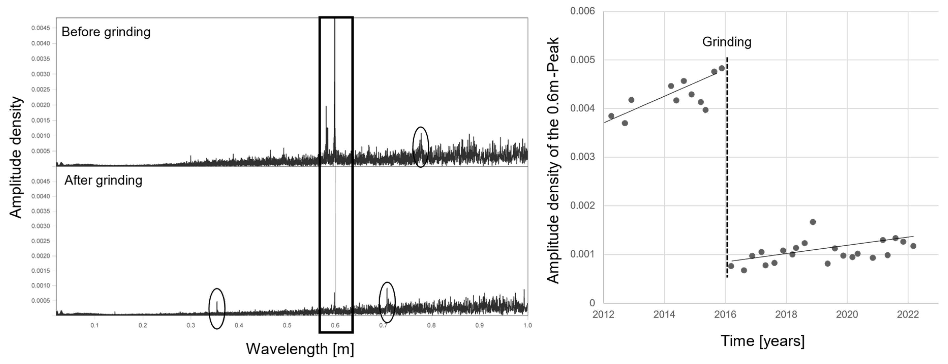
The second aspect relates to the data characteristics of the deconvolved data. The analysis of the surface data in the frequency domain clearly shows a dominant peak in the frequency corresponding to a wavelength of 0.6 m (left part of Figure 9).

A distance of 0.6 m corresponds to the sleeper spacing in Austria. The variety of stiffness between the areas directly above a sleeper and the areas between the sleepers appears to result in wave-like wear of the rail surface. The dominant peak is visible before and after an executed grinding operation, however the severity of the peak differs, as it is significantly reduced by grinding. A further significant smaller peak at 0.78 m before the grinding cannot yet be assigned to an effect. After grinding, two additional peaks (0.35 and 0.71 m) are visible in the frequency spectrum. The 0.71-peak is twice as high as the 0.35-peak, but this is most likely due to the effect that longer wavelengths naturally go hand in hand with a higher amplitude density (which is also clearly shown by the spectral values increasing to the right). Since these peaks occur directly after the grinding, a connection with the grinding process itself is suspected, but a final explanation cannot yet be given. Further analysis was carried out to ensure that the effect was genuinely caused by the rail surface geometry and not by excitations of the track recording vehicle. For this, the magnitude of the 0.6 m peak is used as a quality index and presented over time. The result of the evaluation is shown on the right-hand side of Figure 9. It can be seen that the height of the peak increases linearly from 2012 to 2016, followed by a significant reduction in the peak after grinding. After that further linear growth of the index can be observed. Two conclusions can be deduced from this behaviour. (1) It seems actually be the case, that varying degrees of wear between spots above sleepers and spots between sleepers lead to corrugation like waves in the rails surface. (2) Grinding leads to a significant reduction of these waves. It should be noted that this is not a typical case of corrugation, as the amplitudes of the effects are very small and would not be classified as corrugation by infrastructure mangers. Rather, it is a fundamental oscillation within the rail surface geometry that can be seen anywhere in the network. Further research into the influence of this fundamental oscillation on the wheel–rail contact could prove interesting in terms of energy consumption and noise generation.

2.7. Correlation of Rail Surface Irregularities with Longitudinal Level

After the successful deconvolution of the chord values, the evaluation described in detail in [20] can be repeated using signals without any distortion. Evaluations are performed for four sections with different boundary conditions. Section 1 is a typical mixed traffic line, operated by both passenger and freight traffic, with a maximum permissible speed of 160 km/h (passenger). The second section is mainly used by freight trains and only partly by passenger trains (maximum speed of 130 km/h). The third section represents a mountain line heavily used by long-distance passenger services, local passenger services, and freight services. The maximum speed is 60 km/h (sometimes 80 km/h) due to the tight curves. The fourth section is used by high-speed trains with a maximum speed of 200 km/h and 220 km/h, respectively. As these sections are subject to stricter maintenance guidelines, short-wave effects with high amplitudes are rarely detectable, requiring a correspondingly large data base for reliable results. With the data available, this was only possible by combining sections from different parts of the network, including tunnel sections. The four sections have a total length of approximately 148 km, providing a sufficiently large population. Figure 10 shows the correlation between rail surface irregularities and track geometry quality, based on chord values (original article) and deconvoluted data.

The x-axis presents the minimum amplitude of rail surface irregularities considered in the evaluation. The y-axis shows track geometry quality of spots with rail surface irregularities in percentage to the average quality of the respective section. The quality of the track geometry is described by the standard deviation of the longitudinal level (3–25 m) with a window size of 20 m. The 20 m window size represents a good compromise between the mathematical correctness of the standard deviation calculation and the possibility of describing spot effects. Percentages are obtained by setting the standard deviation value of the longitudinal level at a specific point (spots with rail surface irregularities) in relation to the mean standard deviation value of the respective line. The average quality does not represent the entire network but rather the respective line section (in this case one of four). The value of 100% refers to average quality of the respective section; 200% refers to the standard deviation values, which are twice as high as the respective average. The dashed lines represent the results based on chord values; the solid lines represent the results based on deconvoluted data. It is evident from the upward trend of the curves, that the correlation between the presence of short-wave effects and the track geometry can be confirmed using deconvoluted data. However, in some cases, the course of the lines has changed. When analysing the section with a permissible speed level of 160 km/h, the horizontal fraction up to 0.15 mm visible in the chord-based correlation (dashed blue line) disappears after deconvolution (solid blue line). This is confirmed by the change in the correlation lines of the other sections, especially for the high-speed section (green lines). For the high-speed section, the maximum negative effects on the track geometry are also more pronounced based on the deconvoluted data. Here track geometry exhibits values up to 220% if short-wave effects of high severity are present. The higher the speed level, the greater the negative effect of short-wave effects. This is due to two mechanisms. (1) A higher permissible speed requires a higher quality level of track geometry. As the shown lines represent the ratio between track geometry quality directly under short-wave effects and the average track geometry quality of the analysed section, stricter quality levels lead to higher ratios. (2) Higher permitted speeds lead to higher dynamic force inputs and therefore higher negative effects on track geometry. This is also true for the lower speed levels (60–160 km/h), but their ratios are at a similar level. This allows averaging the results of these three tracks.

3. Results

This paper results in comparing the impact of short-wave effects on longitudinal level based on original chord values and on deconvoluted data. Figure 11 thereby averages the correlation lines for sections with permitted speeds of 60 to 160 km/h. Comparing both lines, the general conclusion of the original paper stays valid by using deconvoluted data. Short-wave effects have a significant impact on track geometry deterioration. However, the detailed course of the correlation lines differs. While using chord-based data for short-wave effects shows a negative impact of short-wave effects with amplitudes bigger than 0.15 mm, using deconvoluted data shifts the critical amplitude down to 0.08 mm (intersection of the quality curve with the horizontal 100% line). The impact of short-wave effects is even more severe than indicated when using chord values, especially in the 0.08…0.3 m range. While the pre-proposed chord-based approach results in the same general conclusion, for detailed evaluations, the deconvolution process is mandatory.

4. Discussion and Outlook

Deconvolution of the rail surface signal leads to slightly adapted results than shown in the original paper; however, it confirms the impact of short-wave effects on track geometry deterioration. While the results of the original paper were not directly transferable to other countries, this is possible now, as deconvoluted data can be compared with geometry measurements of other measurement systems. However, some further research is necessary for final conclusions, as several influencing factors are not dealt with. By correlating the data of a single measurement run, track quality at the time of the measurement run is evaluated. The link between severity of short-wave effects and track geometry quality at a certain point in time is, to some extent, random. For example, a grinding action directly before the measurement reduce/remove short-wave effects, while the consequence of the effects, poor track geometry, is still present. Tamping, on the other hand, reduces poor track geometry while short-wave effects are still remaining. By using a sufficiently big dataset, random effects are tackled; however, future research should be based on time series incorporating deterioration rates and executed maintenance. At the same time, further system properties and boundary conditions impact the relationship between rail surface irregularities and the deterioration of track geometry. Different vehicles (axle load and unsprung mass) with different speeds lead to varying dynamic forces and therefore impact track response. The same is true for different track components. The design of a track and the quality of its components influence the resistance against dynamic loads. Further research should consider these factors by calculating forces caused by a given rail surface irregularity and a given vehicle and correlating these forces with deterioration rates of track geometry.

5. Summary

This paper can be seen as an update of a previously published paper and deals with the impact of rail surface irregularities on the deterioration of track geometry. The assessment of short-wave effects is based on data from an existing measurement system mounted on ÖBB’s measurement car. The system is chord-based, delivering distorted amplitudes depending on the wavelength of the effect. In the original paper, these chord values were used unchanged for a correlation analysis with track geometry, resulting in a clear correlation between short-wave effects and track geometry quality. This paper presents two approaches to negate the signal distortion (deconvolution). Not only do the mathematical and signal processing approaches produce virtually the same results, but the results also agree very well with additional stationary measurements. Repeating the evaluation of the original paper using deconvolved data confirms and even strengthens the correlation between short-wave effects and track geometry quality but leads to partially different conclusions. While the use of chord-based data for short-wave effects shows a negative impact of short-wave effects with amplitudes greater than 0.15 mm, the use of deconvoluted data shifts the critical amplitude down to 0.08 mm. It can be seen that the impact of short-wave effects is even more severe than indicated using chord values straight away. Severe short-wave effects with amplitudes greater than 0.3 mm lead to 50% worse than average track geometry for speeds up to 160 km/h and up to 120% worse for speeds above 200 km/h.