Service Life Evaluation of Curved Intercity Rail Bridges Based on Fatigue Failure

Abstract

There are curved bridge structures in the intercity rail line. During the operation of bridges, they are subjected to train loads, resulting in stress amplitudes of the construction materials; during operation, when the train interval is short, the fatigue performance of the bridge should be emphasized. Unlike straight bridges, when a train travels on a curved bridge, it tends to move in the original direction, which undoubtedly causes the train to deviate from the track. Therefore, it is necessary to set the track deflection to limit this movement trend, which will also impart radial forces on the track structure, and the reaction force of this force is called centripetal force. Under the action of centripetal force, the train generates a virtual force called centrifugal force. The material stress amplitude caused by centrifugal force and the vertical force both need to be considered. Therefore, a curved train–bridge coupled system was established to simulate the dynamic stress of the train passing through a curved bridge, and the stress amplitude and cycle number of the dynamic stress time–history curve were analyzed based on the rain-flow method. The cumulative damage of the bridge under different curve radii, different train speeds, different lengths of span, and different operation interval times was analyzed, and the fatigue life was calculated. The results show that the influence of centrifugal force at a small curve radius cannot be ignored. In addition, the cumulative damage and service life are greatly affected by the train speed and bridge span; especially when the train speed is close to the resonance speed, the service life is significantly reduced. Finally, the recommended values for the train passing speed for curved bridges with different spans are given. It was suggested that the design speed of a curved bridge with a span of 25 m, 30 m, and 35 m should be set in the range of 70 to 106 km/h, 78 to 86 km/h, and about 75 km/h, respectively.

1. Introduction

Intercity rail transit has become an important infrastructure in modern rail transit, with the use of bridges in addition to underground tunnels. Rail bridges have the characteristics of excellent track smoothness, high stiffness, and relatively low cost.

When trains pass through bridges, the bridges will have dynamic responses. Although the amplitude is small, the operating time of the line is long and the frequency of trains passing by is high, which means that there are high requirements for the fatigue resistance of bridges. Therefore, it is usually necessary to focus on the material stress amplitude of the bridges in the design.

The fatigue problem of railway bridges is of interest to many scholars. For example, Song et al. [1] conducted experimental research on the fatigue performance of reinforced concrete slab beams. A corrosion fatigue life assessment method for railway RC girders under combined carbonization and train loads was proposed. They took an existing heavy-duty railway bridge with an 8 m span RC plate beam as an example, and the effects of the annual freight volume, axle weight, and carbonization environment level on its corrosion fatigue life were analyzed. Zhao et al. [2] conducted a 1/4 scale test on a prestressed simply supported concrete box girder of the CRTS-II ballastless track. A series of fatigue tests were conducted on the structural system, and the cumulative fatigue damage results showed that the box beam suffered the greatest damage, followed by the CA mortar, bottom plate, and track plate. The expected remaining lives were 73.67%, 92.90%, and 99.99% of the total fatigue life, respectively. Therefore, in the maintenance and repair of high-speed railway track bridges, the fatigue damage of the box girders should be given specific attention.

In order to detect the stiffness degradation caused by fatigue crack initiation and propagation, Rageh et al. [3] proposed an automatic damage detection framework, which was based on orthogonal decomposition and artificial neural networks, to identify the damage location and strength under non-stationary unknown train loads. The bridge calculation model was used to simulate damage scenarios and train artificial neural networks. The results indicated that the degree of model uncertainty has a significant impact on the efficiency and accuracy of damage detection methods.

With the increase in freight volume and speed on heavy-duty railways, the impact of train loads on orthotropic steel bridge surfaces significantly increases, resulting in fatigue damage to bridges. Therefore, Feng et al. [4] conducted dynamic response and fatigue assessments of the orthotropic steel deck on heavy-duty railway bridges based on train track–bridge coupling analysis and hot spot stress methods. Horas et al. [5] proposed a comprehensive fatigue analysis method for existing metal railway bridges, gradually implementing fatigue assessment methods from the global to local scale, with each requiring varying degrees of computational detail. The former was mainly used to screen fatigue critical connections using single bond curves based on nominal stress, which often oversimplifies the characteristics of load transfer mechanisms and relies on high safety factors. On the other hand, the latter method has been innovatively proposed to refine the fatigue assessment of connections with unsatisfactory residual fatigue life based on overall evaluation.

In the planning of the line, there may be curved bridge forms, as shown in Figure 1. When a train passes through a curved bridge, the train will attempt to continue moving along the tangent direction of the curve (i.e., the direction the train is traveling), so it is necessary to set a track superelevation to form a deflection angle, forcing the train to move along the curve and thereby forming a centripetal force on the train from the track structure. The force exerted by the track on the train will form a reaction force acting on the track. Therefore, when a train crosses a bridge, the bridge not only needs to withstand the vertical load of the train but also needs to withstand the centrifugal reaction force; specifically, under the action of centrifugal reaction force, the bridge will be impacted and even resonate [6,7,8,9], and the combination of these two factors places higher requirements on the fatigue resistance characteristics of the bridge.

In previous engineering applications and research, the fatigue performance of curved bridges has not been given sufficient attention. In order to investigate the fatigue problem of curved bridges under train action, this paper will elaborate and analyze the following aspects: firstly, a curved train–bridge coupled system model was established, and the effectiveness of the model was verified through on-site vibration measurements of the train; secondly, according to the dynamic response of the bridge, the stress state of the material was derived, and the stress amplitude and number of cycles of the bridge material under train dynamic action were derived using the rain-flow counting method; thirdly, taking an actual bridge as the background, the vibration characteristics and resonance speed were calculated to provide a theoretical basis for subsequent analysis; fourthly, key indicators such as the time history response, stress amplitude, and cumulative damage of the bridge under train loads were analyzed; finally, the bridge life was evaluated at various speeds and train intervals. The relevant conclusions can provide assistance for engineering design.

2. Dynamic Stress Calculation of Bridges

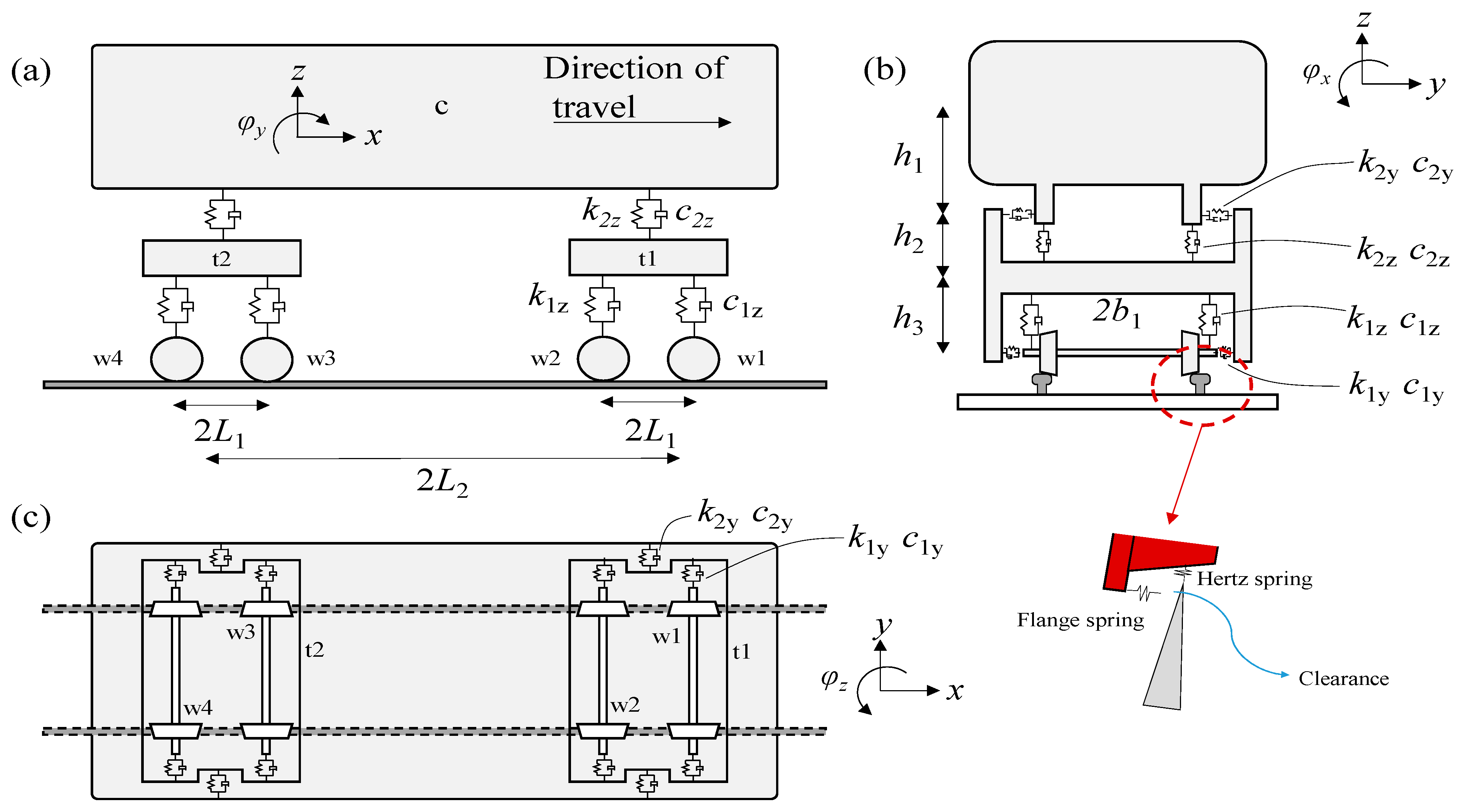
2.1. Curved Train–Bridge Coupled System

When a train passes through a bridge, it will interact with the track–bridge system, resulting in train–bridge coupled vibration. For a straight bridge, the train track–bridge system is symmetrical, including symmetrical trains, symmetrical tracks, symmetrical bridges, and symmetrical loads. For curved track bridges, when a train passes through a curved bridge, it will attempt to move forward in the original direction, which is the tangent direction of the curve. This will undoubtedly cause the train to leave the track, and the track needs to be deflected to resist the train’s departure from the track. Under the action of the centripetal force generated by the track deflection, the train will experience a virtual force called centrifugal force, which is used to balance the centripetal force, and this is an inertial force that can be applied to the center of mass position of the car bodies, bogies, and wheelsets in numerical models.

To more accurately describe the dynamic response of curved bridges under train load, a curved train–bridge coupled system model (CTBCSM) was established based on a symmetrical system. The train was simulated using a mass spring damping model [10,11], as shown in Figure 2, where c denotes the car-body; t₁ and t₂ denote the front and rear bogies; w₁, w₂, w₃, and w₄ denote the first, second, third, and fourth wheelsets, respectively; k denotes the stiffness, and its first subscript y or z denotes the lateral and vertical direction, while its second subscript 2 or 1 denotes the secondary or primary suspension; L₁ denotes the half distance between two wheelsets; L₂ denotes the half distance between two bogies; h₁, h₂, and h₃ denote the vertical distance between the center of the car-body and secondary suspension, between the secondary suspension and the center of the bogie, and between the center of the bogie and the wheelset. The train body, bogie, and wheelset were considered rigid bodies, and the suspension was considered spring damping. Based on the principle of constant elastic potential energy, the dynamic equation of the train can be obtained as follows:

$$M^V{\ddot{X}}^V+C^V{\dot{X}}^V+K^V{X}^V=F^V,$$

(1)

where M^V is the mass matrix of the train, and it can be written as follows,

$$M^V=\mathrm{diag}[M^{V1} M^{V2}\cdots M^{Vn}]$$

(2)

with

$$M^{Vi}=\mathrm{diag}[M^c M^{t1} M^{t2} M^{w1} M^{w2} M^{w3} M^{w4}],$$

(3)

$$M^c=\mathrm{diag}[m_c m_c J_{cx} J_{cy} J_{cz}]$$

(4)

$$M^{ti}=diag[m_t m_t J_{tx} J_{ty} J_{tz}]$$

(5)

$$M^{wi}=\mathrm{diag}[m_w m_w J_{wx} J_{wy} J_{wz}],$$

(6)

where m and J denote the mass and moment of inertia, respectively, and the subscripts c, t, and w denote car-body, bogie, and wheelset, respectively.

K^V is the stiffness matrix of the train, and it can be written as follows,

$$K^V=diag[K_{v1} K_{v2}\cdots K_{vn}],$$

(7)

$$K^{Vi}=\left[\begin{array}{ccccccc}{K}_c& & & & & & symm.\\ K_{ct1}& K_{t1t1}& & & & & \\ K_{ct2}& 0& K_{t2t2}& & & & \\ 0& K_{t1w1}& 0& K_{w1w1}& & & \\ 0& K_{t1w2}& 0& 0& K_{w2w2}& & \\ 0& 0& K_{t2w3}& 0& 0& K_{w3w3}& \\ 0& 0& K_{t2w4}& 0& 0& 0& K_{w4w4}\end{array}\right]$$

(8)

$$K_c=\left[\begin{array}{ccccc}4k_{y2}& & & & symm.\\ 0& 4k_{z2}& & & \\ 4h_1{k}_{y2}& 0& 4{h_1}^2{k}_{y2}+4{b_2}^2{k}_{z2}& & \\ 0& 0& 0& 4{d_2}^2{k}_{z2}+4{h_1}^2{k}_{x2}& \\ 0& 0& 0& 0& 4{d_2}^2{k}_{y2}+4{b_2}^2{k}_{x2}\end{array}\right]$$

(9)

$$K_{ct1}=\left[\begin{array}{ccccc}-2k_{y2}& 0& -2h_1{k}_{y2}& 0& -2d_2{k}_{y2}\\ 0& -2k_{z2}& 0& 2d_2{k}_{z2}& 0\\ 2h_2{k}_{y2}& 0& d& 0& 2h_2{d}_2{k}_{y2}\\ 0& 0& 0& 2h_1{h}_2{k}_{x2}& 0\\ 0& 0& 0& 0& -2{b_2}^2{k}_{x2}\end{array}\right]$$

(10)

$$K_{ct2}=\left[\begin{array}{ccccc}-2k_{y2}& 0& -2h_1{k}_{y2}& 0& -2d_2{k}_{y2}\\ 0& -2k_{z2}& 0& -2d_2{k}_{z2}& 0\\ 2h_2{k}_{y2}& 0& d& 0& -2h_2{d}_2{k}_{y2}\\ 0& 0& 0& 2h_1{h}_2{k}_{x2}& 0\\ 0& 0& 0& 0& -2{b_2}^2{k}_{x2}\end{array}\right]$$

(11)

$$K_{t1t1}=K_{t2t2}=\left[\begin{array}{ccccc}2k_{y2}+4k_{y1}& & & & symm.\\ 0& 2k_{z2}+4k_{z1}& & & \\ 4h_3{k}_{y1}-4k_{y1}& 0& a& & \\ 0& 0& 0& b& \\ 0& 0& 0& 0& c\end{array}\right]$$

(12)

$$a=2{b_2}^2{k}_{z2}+2{h_2}^2{k}_{y2}+4{b_1}^2{k}_{z1}+4{h_3}^2{k}_{y1}$$

(13)

$$b=2{h_2}^2{k}_{x2}+4{d_1}^2{k}_{z1}+4{h_3}^2{k}_{x1}$$

(14)

$$c=4{b_1}^2{k}_{x1}+4{d_1}^2{k}_{y1}+2{b_2}^2{k}_{x2}$$

(15)

$$K_{t1w1}=K_{t2w3}=\left[\begin{array}{ccccc}-2k_{y1}& 0& -2h_3{k}_{y1}& 0& 2d_1{k}_{y1}\\ 0& -2k_{z1}& 0& -2d_1{k}_{z1}& 0\\ 0& 0& -2{b_1}^2{k}_{z1}& 0& 0\\ 0& 0& 0& 0& -2{b_1}^2{k}_{x1}\end{array}\right]$$

(16)

$$K_{w1w1}=K_{w2w2}=K_{w3w3}=K_{w4w4}=\left[\begin{array}{cccc}2k_{y1}& 0& 0& 0\\ 0& 2k_{z1}& 0& 0\\ 0& 0& 2{b_1}^2{k}_{z1}& 0\\ 0& 0& 0& 2{b_1}^2{k}_{x1}\end{array}\right]$$

(17)

C^V is the damping matrix of the train, and it can be obtained by replacing k or K in the K^V matrix with c or C.

F^V is the load vector of the train, and it includes the wheel–rail contact force and self-load. In addition, in the numerical model, in order to simulate the force generated by the train passing through a curved bridge that deviates from the track trend, the above is called centrifugal force, which is applied to the center of mass position of the car-body, bogie, and wheelset, in the radial direction. This can be stated using Equation (18).

$$F_c={\displaystyle \frac{m_i{v}^2}{R}},$$

(18)

where v is the train’s running (rotational) speed; m_i is the mass of the car-body, bogie, or wheelset; and R is the bridge’s curve radius. The curved bridge will be subject to the reaction force of the train’s centrifugal force, which will result in the corresponding transverse load [12].

The rail and bridge were coupled using the CTBCSM, and the knife-edge wheel rail contact model simplifies the contact into vertical and transverse springs [13,14,15,16]. The Hertz spring’s compression amount can also be calculated by comparing the relative vertical and horizontal displacement of the side wheels [17].

The mass matrix ($M^B$) and stiffness matrix ($K^B$) of the bridge in the global system can be obtained after modeling the bridge using the finite element approach. The bridge, piers, and steel rails were all simulated using Euler beam elements. The fasteners between the steel rails and the bridge were simulated using a spring-damping system. The bearings between the girders and piers were also simulated using spring-damping systems, and the bottom of the piers was consolidated with the ground. The S-N curve was used to estimate the fatigue performance of bridges, which is a semi-theoretical and semi-empirical method that ignores the influence caused by stiffness degradation, and this estimation method was also used by other researchers [1,18].

By assembling the local matrices of stiffness and mass through self-coding, the overall stiffness and mass matrices could be obtained. It was assumed that each order’s damping ratio is 0.03 and that the damping was Rayleigh damping [17]. Equation (2) is the bridge’s dynamic equation.

$$M^B{\ddot{X}}^B+C^B{\dot{X}}^B+K^B{X}^B=F^B,$$

(19)

The dynamic equation of the system can be obtained by combining Equations (1) and (19). The mass, stiffness, and damping of the train and bridge are coupled to each other through the wheel–rail relationship. The system model was completed by autonomous programming, and the dynamic response of each time was calculated by an unconditional explicit integration algorithm [19]. Our previous work [20] can be reviewed for comprehensive details on the process and technique. Due to the fact that this paper mainly focused on the fatigue resistance performance of structures, and the material fatigue performance of structures was mainly related to the magnitude of the stress amplitude and the number of cycles, the material stress caused by the self-weight of bridges could be ignored.

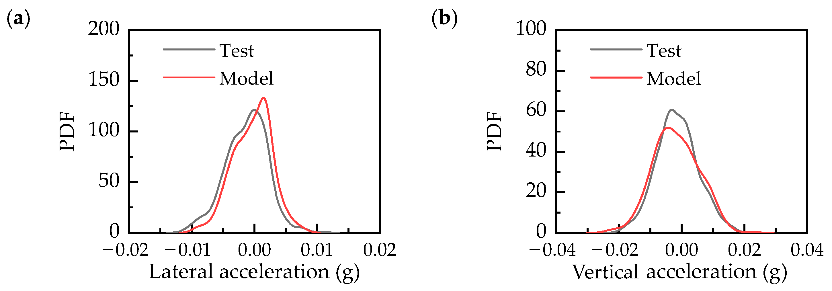
2.2. Validation of CTBCSM

To verify the accuracy of the CTBCSM, on-site testing was conducted on a train to collect the lateral and vertical accelerations of the train car-body. This train was a CRH train, running from Fuzhou to Gutian North in China. The collection device was a wireless acceleration collector provided by WIT company, which can be connected to the terminal through Bluetooth, with a sampling frequency of 100 Hz and an acceleration sampling accuracy of 0.001 g. The acceleration time histories of the front, middle, and rear ends of a carriage of the train were collected. During the collection process, the train speed was not constant, and the speed was about 200 km/h. Due to the testing process passing through the roadbed section, tunnel, and bridge sections, the acceleration responses of the curved bridge section were taken for verification.

The test results and calculation results are shown in Figure 3. For the vertical acceleration time history of the train car-body, it can be seen that it oscillates roughly around zero, with an acceleration range of −0.02 g to 0.02 g; the lateral acceleration of the train car-body was within the range of −0.01 g to 0.01 g. Due to the fact that track irregularity is a random process, the train acceleration is also a random process. Therefore, by comparing the probability density functions (PDFs) of the test results and simulation results, as shown in Figure 4, it can be seen that the simulated PDF curve is very close to the test results. Overall, the model calculation results are very close to the test results in both amplitude and trend, indicating that the CTBCSM can accurately obtain the response of the asymmetric train–bridge system.

2.3. Stress Calculation

The CTBCSM was utilized to calculate the bridge’s dynamic stress response, and the stress under load was typically used to assess the fatigue performance of the part or structure.

In this study, the life of a railway bridge can be predicted from a single calculation of the stress and dynamic response of the steel bars. In fact, this is just a quick evaluation method, and building an appropriate finite element model is required if accurate results are needed, but the computational efficiency is also much worse. Therefore, the slip between the steel bar and the concrete was ignored, and the two were bound together [1,18].

When the reinforced concrete beam is linear elastic, the strain of the steel bar can be estimated by the cross-section deformation of the concrete beam. Although in long-term deformation, the bridge material will be damaged, in short-term deformation under the action of the train load, the bridge still maintains the elastic state [21]; therefore, the strain can be estimated from the beam deformation in subsequent analyses. If both ends of the element are simply subjected to bending moment and shear force, the displacement–strain relationship can be predicted using FEM theory [18,19]. As a result, the strain–strain connection is as follows:

$$\epsilon =B\delta$$

(20)

where $\delta$ is the element node’s deformation, which can be represented as in Equation (21), and $\epsilon$ is the element’s strain.

$$\delta =\left[\begin{array}{cccc}{u}_i& {\theta }_i& u_j& {\theta }_j\end{array}\right]$$

(21)

where u and θ denote the node’s vertical and rotational deformation, respectively. B is the deformation–strain relationship matrix, which specifies the transformation relationship between the strain at any point in the element and the displacement of the node in the element, and it is equivalent to the formula,

$$B=-y{\displaystyle \frac{{\mathrm{d}}^{2}N}{\mathrm{d}{x}^2}}$$

(22)

where N is the form function and y is the distance (including sign) from the strain calculation point to the central axis. B can therefore be translated into the following formula:

$$B=\left[\begin{array}{cccc}{\phi }_1& {\phi }_2& {\phi }_3& {\phi }_4\end{array}\right]$$

(23)

with

$$\{\begin{array}{c}{\phi }_1={\displaystyle \frac{6y}{l^2}}\left(1-2{\displaystyle \frac{x}{l}}\right)\\ {\phi }_2=-{\displaystyle \frac{2y}{l^2}}\left(2-3{\displaystyle \frac{x}{l}}\right)\\ {\phi }_3=-{\displaystyle \frac{6y}{l^2}}\left(1-2{\displaystyle \frac{x}{l}}\right)\\ {\phi }_4=-{\displaystyle \frac{2y}{l^2}}\left(2-3{\displaystyle \frac{x}{l}}\right)\end{array}$$

(24)

where l denotes the length of the element and x denotes the distance between the calculated point and the left node of the element.

After obtaining the strain, the stress can be calculated by the following formula:

$$\sigma =D\epsilon$$

(25)

where D is the matrix of stress–strain relationships. If the material stress–strain relationship D in the long-term operation of the bridge is linear elasticity, D equals the elastic modulus E of the material. Thus, Equation (25) can be rewritten as the following equation,

$$\sigma =E\epsilon$$

(26)

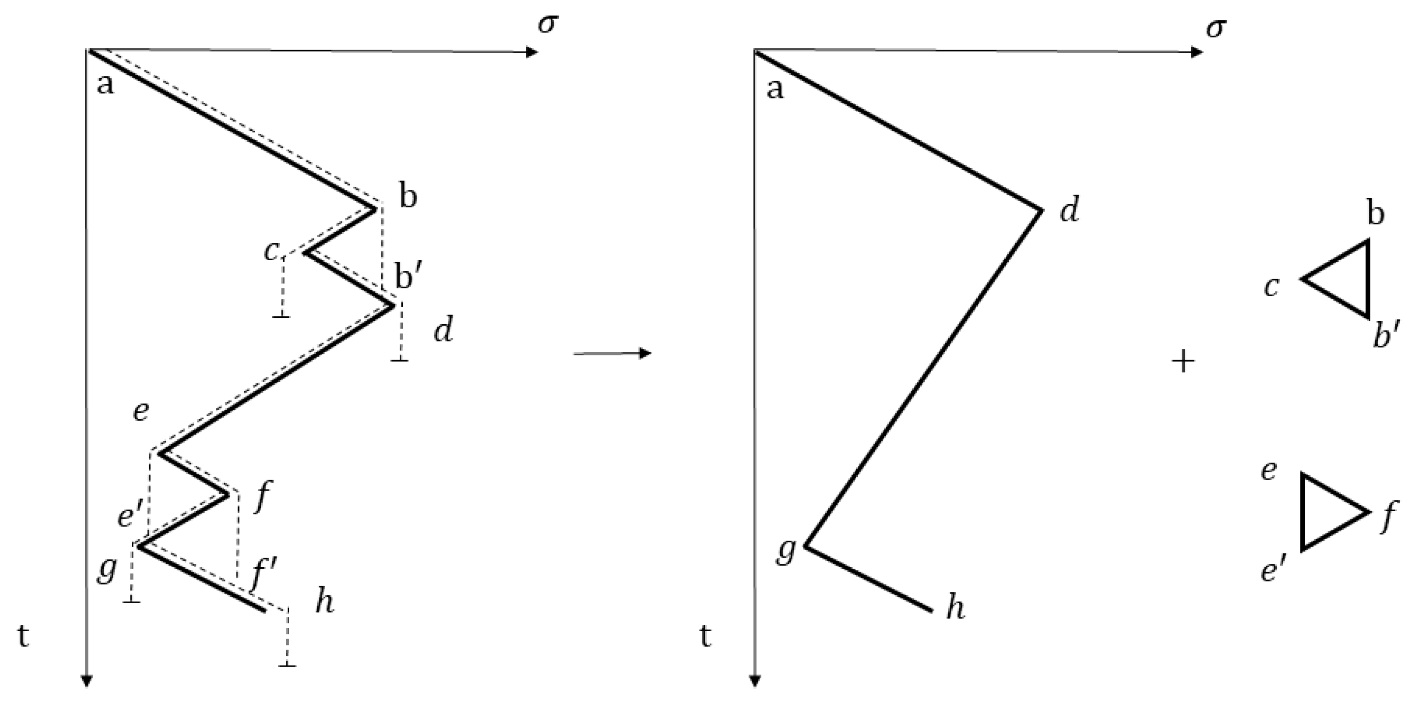
2.4. Stress Amplitude

The S–N curve of the steel rebar is as follows:

$$\lg N=\lg C-m\lg \Delta \sigma$$

(27)

where C and m are the coefficients for steel reinforcement, and according to Song et al. [22], they can be 1.4213 × 10¹⁰ and 1.7637, respectively; $\Delta \sigma$ represents the stress range of the steel reinforcement, and N is the total number of stress cycles.

It is crucial to determine the stress amplitude and cycle count following the creation of the stress time history curve using the CTBCSM. The application of the rain-flow method (Figure 5) can efficiently perform this task. Stress flows like rainwater, first from point a to point b, and then from point b to point c and b′. Subsequently, rainwater flows from point b′ to point d and is directly left behind, while rainwater also flows out directly from point c. The rainwater at point b flows to e-e′-g and then flows directly out. Throughout the process, large stress amplitudes of a-d-g-h and small stress amplitudes of b-c-b′ and e-f-e′ were formed. In this way, the stress process can be decomposed into several stress amplitudes. Additional information regarding the rain-flow process can be found in Ref. [21].

Once stress amplitudes and their corresponding cycle times are obtained, the equivalent stress amplitude can be calculated using the following formula.

$$S_{re}\left(t\right)={\left({\displaystyle \sum \frac{n_i{\left(\Delta {\sigma }_i\left(t\right)\right)}^m}{{\displaystyle \sum n_i}}}\right)}^{1/m}$$

(28)

where n_i denotes the cycle number of the i-th stress amplitude.

Substituting Equation (11) into Equation (10), the number of cycles of equivalent stress amplitude during fatigue failure of steel bars can be obtained, and according to Miner [23], the fatigue damage D_s(t) to reinforcement resulting from a single train passing can be computed using the subsequent formula.

$$D_s\left(t\right)={\displaystyle \frac{S_{re}^m\left(t\right){\displaystyle \sum n_i}}{C}}$$

(29)

Over an extended period of operation, the cumulative fatigue damage to a bridge increases consistently with its service time. Following M years of operation, the formula below can be used to compute the cumulative fatigue damage (D_t) to the bridge.

$$D_t={\displaystyle \sum _{g=1}^M{D}_{s,j}\left(t\right)N_y}$$

(30)

where N_y represents the annual number of trains passing over the bridge.

3. Case Study

A curved concrete track bridge situated in Zhengzhou, China, was used as a case study for analysis. The bridge had a curve radius of 800 m and spanned 25 m. The concrete used had a strength grade of C60, and an elastic modulus of 3.45 × 10¹⁰ Pa, while the steel reinforcement bars were HRB400 grade. The bridge track had a box-shaped cross-section with a horizontal section moment of inertia Iy = 1.3514 m⁴ and a vertical section moment of inertia Iz = 9.1108 m⁴. The density of the track bridge was 2.85 × 10³ kg/m³, and its cross-sectional area was 3.6552 m². By solving the eigenvalues and eigenvectors of the stiffness matrix K and the mass matrix M, the corresponding natural frequency of the structure can be obtained.

Table 1. Natural vibration frequencies of bridge.

Order	Vertical	Lateral
1st	5.30 Hz	13.73 Hz
2nd	21.16 Hz	54.89 Hz
3rd	47.59 Hz	123 Hz

provides the natural vibration frequencies of the bridge, while

Table 2. Parameters of train.

Symbol	Meaning	Value
mc	Mass of car-body	21,920 kg
mt	Mass of bogie	2550 kg
mw	Mass of wheelset	1420 kg
2L1	Spacing of two wheelsets	2.2 m
2L2	Spacing of two bogies	12.5 m
Lv	Length of carriage	19 m

presents the train parameters. For simply supported girders, the maximum deformation occurs in the middle of the girder span, that is, the stress of the steel bar at the bottom of the beam span is the greatest; thus, in the subsequent analysis, the stress was the stress of the steel bar at the bottom of the girder span. In the calculation and analysis, four bridge spans of 600 m, 800 m, 1000 m, and 1200 m were considered. Since the intercity train was a low-speed train, the curve radius of 1200 m was large, and the bridge can be considered as a straight bridge.

To analyze the fatigue life of curved bridges more systematically, the analysis of curved bridges with spans of 20 m, 30 m, and 35 m was supplemented. Since the bridge will produce a resonance effect at a specific speed, according to Yang et al. [24], the train resonance speed $v_n^i$ of a railway bridge can be calculated by the following formula,

$$v_n^i=3.6{\displaystyle \frac{f_n^B{L}_v}{i}} \mathrm{km}/\mathrm{h}$$

(31)

where $f_n^B$ denotes the natural frequency of the bridge; L_v denotes the length of the carriage; i denotes the i-order resonance. After calculation, the first four order resonance speeds of bridges with different spans are shown in

Table 3. Resonance train speed.

Length of Span	i = 1	i = 2	i = 3	i = 4
20 m	566 km/h	283 km/h	189 km/h	141 km/h
	2261 km/h	1131 km/h	754 km/h	565 km/h
	5083 km/h	2541 km/h	1694 km/h	1271 km/h
25 m	363 km/h	181 km/h	121 km/h	91 km/h
	1447 km/h	724 km/h	482 km/h	362 km/h
	3255 km/h	1628 km/h	1085 km/h	814 km/h
30 m	252 km/h	126 km/h	84 km/h	63 km/h
	1005 km/h	503 km/h	335 km/h	251 km/h
	2261 km/h	1131 km/h	754 km/h	565 km/h
35 m	185 km/h	92 km/h	62 km/h	46 km/h
	739 km/h	369 km/h	246 km/h	185 km/h
	1661 km/h	831 km/h	554 km/h	415 km/h

.

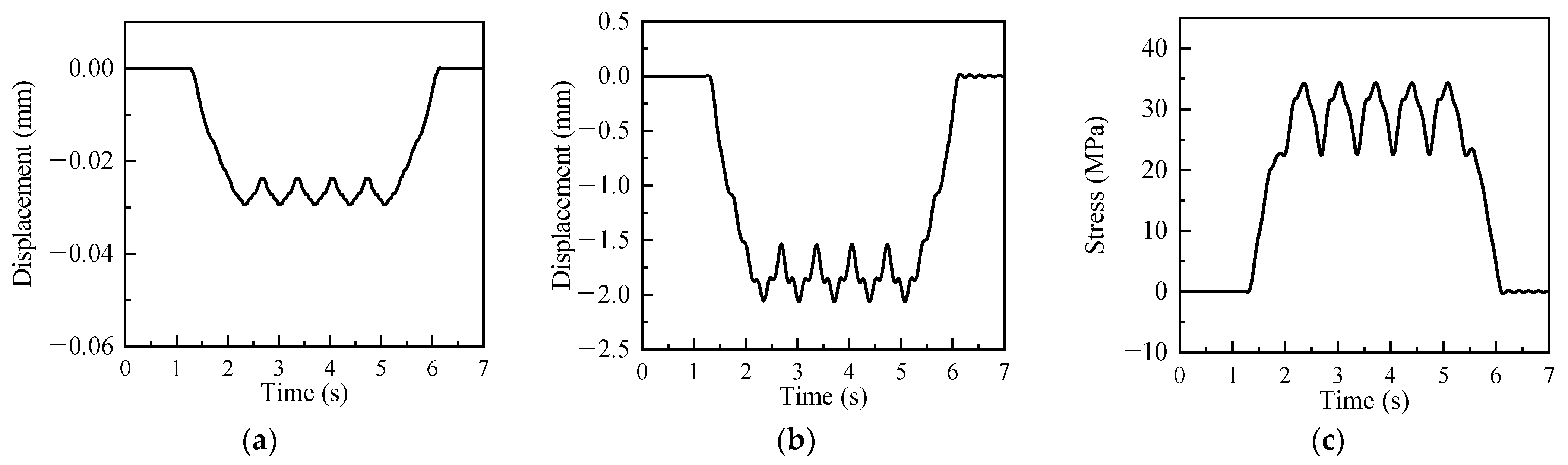
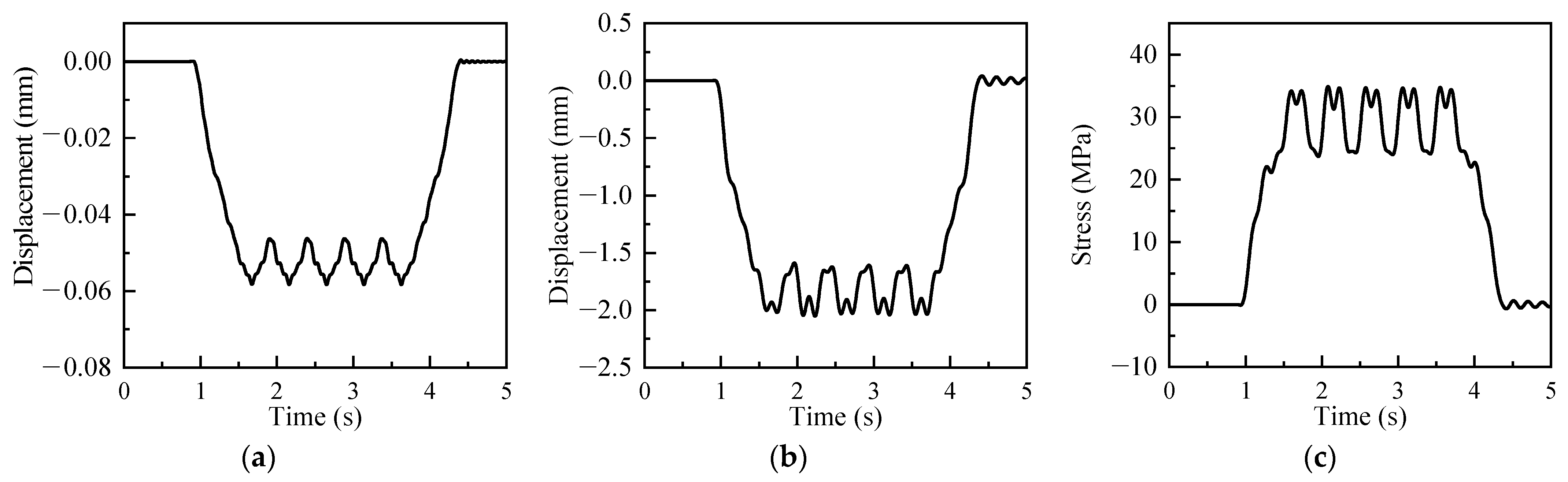
3.1. Time History Response

The dynamic time history curve of a bridge with a curve radius of 800 m and a train speed of 100 km/h is displayed in Figure 5. Five displacement peaks are visible in response to the bridge span’s lateral and vertical displacement in Figure 6a,b. This is because, although the train consists of a total of six carriages, including five sets of such concentrated loads, the four wheelsets of two adjacent bogies in the adjacent cars are more concentrated, akin to a set of concentrated loads. The maximum stress time history curve for bridge steel bars is displayed in Figure 6c. Due to only discussing the structural fatigue performance, the self weight of the bridge was neglected, and the initial stress value is zero. The displacement time history and the maximum stress value, which is around 35 MPa, exhibit a similar trend.

The dynamic time history curve of a bridge with a curve radius of 800 m and a train speed of 120 km/h is depicted in Figure 7. While the vertical displacement peak is not obvious, Figure 7a depicts the bridge midspan’s lateral reaction, which includes five displacement peaks. The bridge steel bars’ maximum stress time history curve is depicted in Figure 7c. When the train is running at a speed of 120 km/h, the stress time history curve is more asymmetrical than it is at 100 km/h.

Figure 8 displays the dynamic time history curve for a bridge with a train speed of 140 km/h and a curve radius of 800 m. The bridge span manifests five peaks in both the transverse response and vertical displacement, and the curve has a comparatively smooth trend. Figure 8c demonstrates the time history curve of maximum stress experienced by the bridge reinforcement, and it follows a similar trend to the vertical displacement.

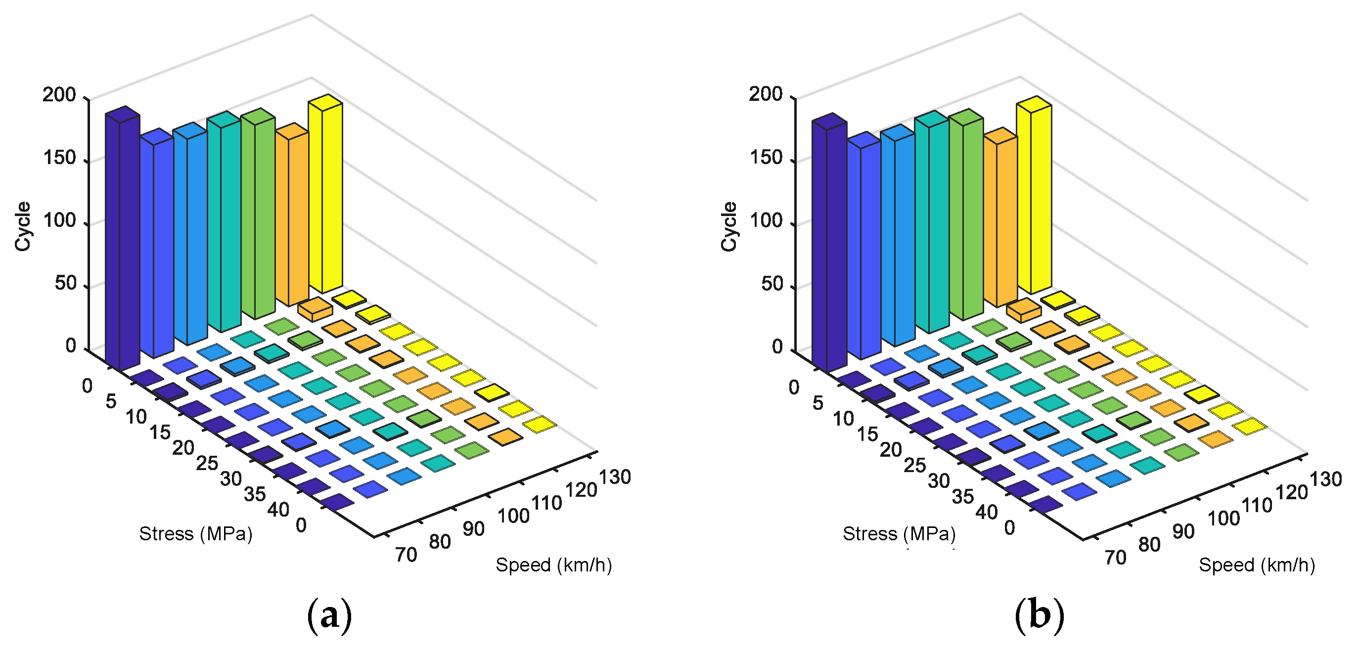
3.2. Stress Amplitude

Using the rain-flow approach, the stress amplitude of the steel bar and the associated cycle periods of the train going through the bridge were determined. The results when considering stress amplitudes with spans of 25 m, 30 m, and 35 m at various train speeds are displayed in Figure 9, Figure 10 and Figure 11.

Figure 9 illustrates how little the fatigue stress amplitude and cycle periods of the bridge change under various curve radii. Furthermore, the stress amplitude at varying speeds is primarily centered within 5 MPa, and as the speed increases, the stress amplitude below 5 MPa progressively diminishes. This is because the train’s passage through the bridge is comparable to a number of moving loads doing so. Even though there are several loads in motion, they are all moving relatively near to one another. There are more small stress amplitudes brought on by bridge vibration than huge stress amplitudes.

As demonstrated in Figure 10, the number of stress amplitudes within 5 MPa progressively reduces with an increase in train speed when the span is 30 m, comparable to the span of 25 m. There is no clear relationship between the change in speed and the change in stress amplitude when the span is 35 m.

It is evident from a comparison of Figure 9, Figure 10 and Figure 11 that the bridge span significantly affects the curved bridges’ stress amplitude. For instance, the stress amplitude of 5–10 MPa is not as great when the span is 25 m, but it is considerably higher when the span is 35 m.

Comparing different spans, it can be seen that the span has a great impact on the stress amplitude and the number of cycles; for example, when the curve radius is 1200 m, with an increase in the span, the number of cycles in the small stress range (0–5 MPa) is significantly reduced, and the number of cycles in the stress range of 5–30 MPa is significantly increased.

3.3. Cumulative Damage

The action of the train load will cause damage to the bridge; a single damaging event is not substantial, but cumulative damage over time will result in significant harm. The cumulative damage of curved bridges with train operation intervals of 4 min, 6 min, and 8 min (curve radius of 800 m) was calculated in order to discuss the cumulative damage of bridges with different spans and train speeds. The results are displayed in Figure 12, Figure 13 and Figure 14.

There is no discernible relationship between the cumulative damage and the bridge span, but the cumulative damage law of various train operation time intervals is similar. The cumulative damage also exhibits an exponential growth pattern with an increase in operation duration. For instance, the bridge’s 30 m span has the highest cumulative damage growth rate when the train travels at 80 km/h. Due to its proximity to the third resonance speed of 84 km/h of the bridge with a span of 30 m, the bridge with a span of 25 m has the smallest cumulative damage increase rate.

However, when the train speed is 100 km/h, the cumulative damage growth rate of the bridge with a span of 35 m is the largest, while the cumulative damage growth rate of the bridge with a span of 25 m is the smallest, because the train speed of 100 km/h is close to the second resonance speed of the bridge with a span of 35 m.

When the train speed is 120 km/h, the cumulative damage growth rate of the bridge with a span of 25 m is the largest, while the cumulative damage growth rate of the bridge with a span of 20 m is the smallest, because the train speed of 120 km/h is close to the third resonance speed of the bridge with a span of 25 m. This shows that the bridge span and train speed have a great influence on cumulative damage, mainly because the bridge span affects the natural vibration frequency of the bridge, and the train speed affects the excitation frequency of the train to the bridge.

In addition, as shown in Figure 13 and Figure 14, the cumulative damage to the bridge will be alleviated if the train operation interval is increased.

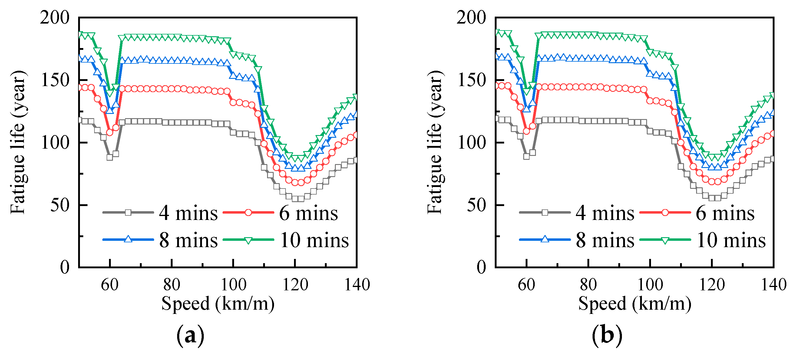
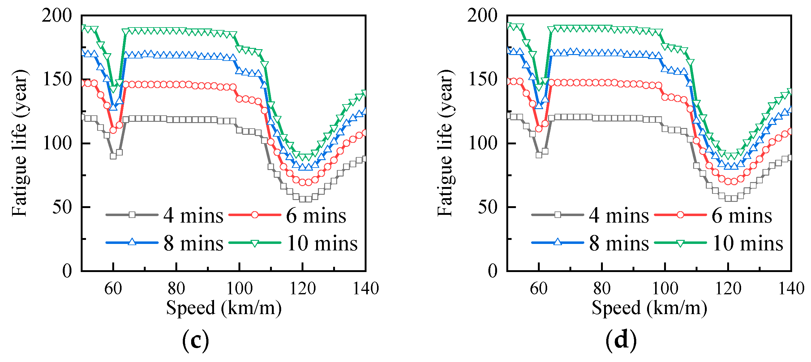
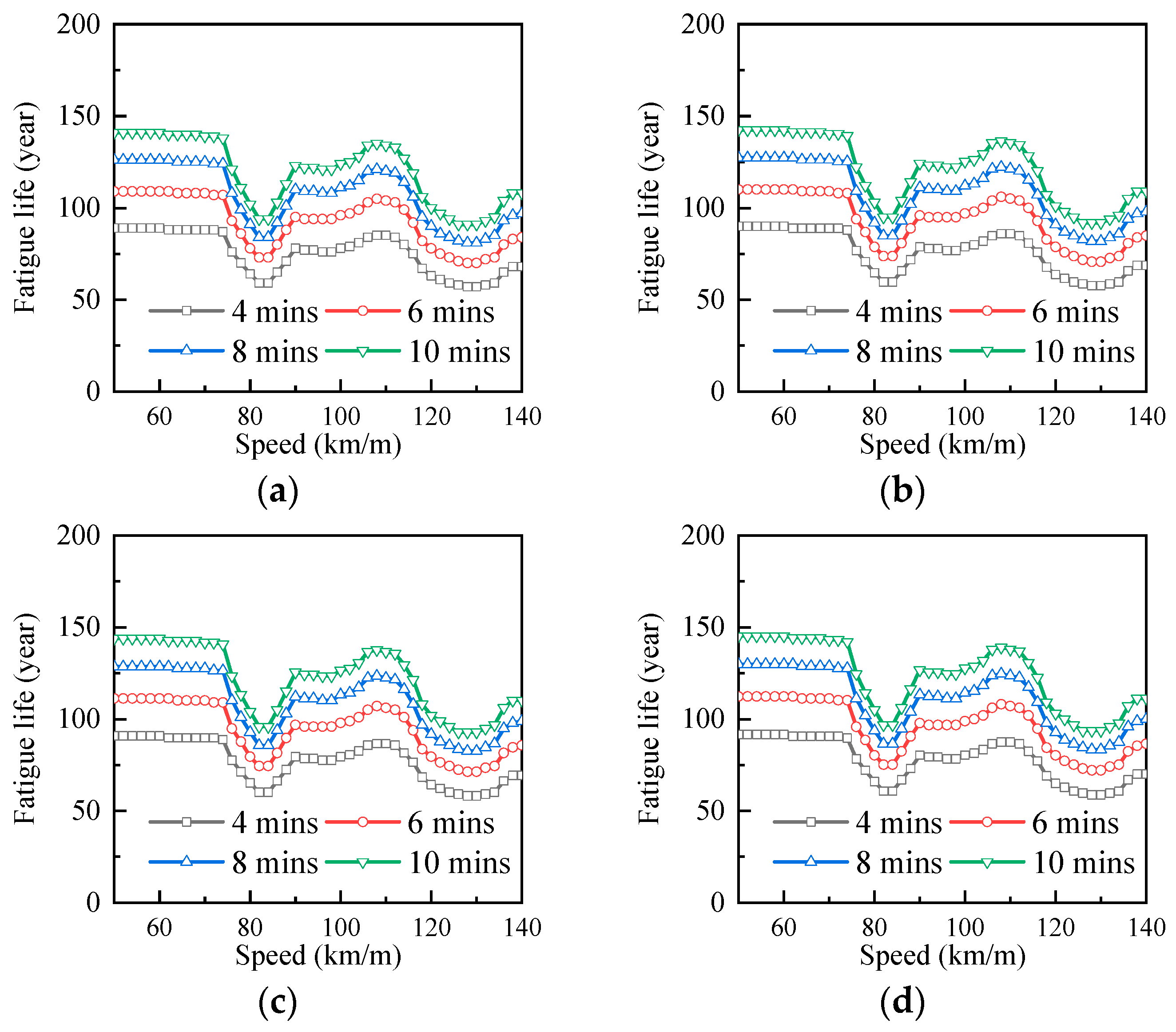
3.4. Evaluation of Lifetime

In order to better accurately depict the curved bridge’s fatigue performance, the fatigue life of the structure under various curve radii was computed. Figure 15 displays the fatigue life values for the 20 m span bridge. It is unclear how the train speed and curve radius affect the fatigue life. Furthermore, the fatigue life of the bridge can be efficiently increased by increasing the train interval time. In addition, different curve radii have almost no effect on the fatigue life because the fatigue life depends on the transverse and vertical deformation of the girder. While the curve radius has a greater effect on the transverse deformation, the transverse deformation is much smaller than the vertical deformation.

Figure 16 displays the bridge’s fatigue life results over a 25 m span. When the train is traveling between 50 and 60 km/h, the fatigue life generally falls as the train speed increases. The fatigue life increases as the speed rises when it is between 60 and 70 km/h. A fatigue life of 70 to 106 km/h is considered stable at such a pace.

The fatigue life initially falls at speeds higher than 100 km/h and then gradually increases as the speed rises, reaching a low point at 120 km/h. This is due to resonance effects caused by the speed of 120 km/h being near the bridge’s third resonance speed. Additionally, when the train interval times grow, the fatigue life of the bridge diminishes, and the fatigue life is slightly impacted by changes in the curve radius. It is advised that the design speed for curved bridges with a 25 m span be within the range of 70 to 106 km/h. Similarly, it can be seen that the curve radius has little effect on the fatigue life.

Figure 17 displays the fatigue life results for the 30 m span bridge. Generally speaking, the fatigue life is not affected much by the speed when it is between 50 and 74 km/h. However, when the speed surpasses 74 km/h, the fatigue life initially falls and then rises as the speed increases, with the low point appearing around 82 km/h. This is because the speed is getting close to the bridge’s third resonance speed, which is 84 km/h. The fatigue life gradually grows with speeds over 90 km/h and gradually diminishes with speeds above 110 km/h. It is advised that the operating speeds for curved bridges with a span of thirty meters stay outside of the range of 78 to 86 km/h. Similarly, it can be seen that the curve radius has little effect on the fatigue life.

Figure 18 displays the fatigue life results across a 35 m span. As can be observed, the fatigue life in the same example rises as the train operation interval does, corresponding with the real world. Generally speaking, as the train speed increases to between 50 and 62 km/h, the fatigue life declines. The fatigue life rises as the train speed increases to between 62 and 75 km/h. The speed of 62 km/h is the lowest of them all since it is the bridge’s third resonance speed, which generates the resonance effect.

The fatigue life diminishes when the train speed increases to between 75 and 88 km/h. The fatigue life rises with a train speed in the 88–140 km/h range; however, the increase is not significant. It is advised that the 35 m span curved bridge’s design speed be close to 75 km/h. Similarly, it can be seen that the curve radius has little effect on the fatigue life.

4. Conclusions

To fully grasp the anti-fatigue performance of intercity curved bridges, a curved train–bridge coupled system model was established, in which the train was simulated by a multi-rigid body, the track-bridge system was simulated by the finite element method, and the system influence caused by the curved line was simulated by applying centripetal and centrifugal forces. The dynamic stress amplitude of the bridge and the corresponding cycle number were obtained by the rain-flow method, and the stress dynamic time history response, stress amplitude, cumulative damage, and fatigue life of the reinforcement were analyzed. The results are as follows:

(1)

The stress amplitude of the reinforcing bars of the bridge was mainly concentrated within 10 MPa, which was mainly due to the control of vertical load. However, the influence of centrifugal force in the case of a small curve radius and large train speed could not be ignored.

(2)

The cumulative damage of a curved bridge presented an exponential growth trend with the increase in operation time, and the shorter the interval time was, the faster the growth rate. The cumulative damage was mainly affected by the bridge span and train speed, especially when the train speed was close to the resonance speed.

(3)

When the bridge span was 20 m, the train speed had little effect on the fatigue life, and the fatigue life increased with the increase in the train operation interval.

(4)

When the bridge span was 25 m, 30 m, and 35 m, the train speed had a great influence on the fatigue life, and at different speed stages, the fatigue life of the bridge changes differently from the train speed, mainly because the dynamic load of the train causes the bridge resonance at some speeds. It was suggested that the design speed of the curved bridge with a span of 25 m should be set in the range of 70 to 106 km/h; the speed of the curved bridge with a span of 30 m was avoided within the range of 78 to 86 km/h; the design speed of the curved bridge with a span of 35 m was set near 75 km/h.

References

1. Song, L.; Cui, C.; Liu, J.; Yu, Z.; Jiang, L. Corrosion-Fatigue Life Assessment of RC Plate Girder in Heavy-Haul Railway under Combined Carbonation and Train Loads. Int. J. Fatigue 2021, 151, 106368. [Google Scholar] [CrossRef]
2. Zhao, L.; Zhou, L.; Yu, Z.; Mahunon, A.D.; Peng, X.; Zhang, Y. Experimental Study on CRTS II Ballastless Track-Bridge Structural System Mechanical Fatigue Performance. Eng. Struct. 2021, 244, 112784. [Google Scholar] [CrossRef]
3. Rageh, A.; Eftekhar Azam, S.; Linzell, D.G. Steel Railway Bridge Fatigue Damage Detection Using Numerical Models and Machine Learning: Mitigating Influence of Modeling Uncertainty. Int. J. Fatigue 2020, 134, 105458. [Google Scholar] [CrossRef]
4. Feng, Q.; Zhu, Z.; Tong, Q.; Yu, Y.; Zheng, W. Dynamic Responses and Fatigue Assessment of OSD in Heavy-Haul Railway Bridges. J. Constr. Steel Res. 2023, 204, 107873. [Google Scholar] [CrossRef]
5. Horas, C.S.; De Jesus, A.M.P.; Calçada, R. Efficient Progressive Global-Local Fatigue Assessment Methodology for Existing Metallic Railway Bridges. J. Constr. Steel Res. 2022, 196, 107431. [Google Scholar] [CrossRef]
6. Zeng, Q.; Yang, Y.B.; Dimitrakopoulos, E.G. Dynamic Response of High Speed Vehicles and Sustaining Curved Bridges under Conditions of Resonance. Eng. Struct. 2016, 114, 61–74. [Google Scholar] [CrossRef]
7. Wang, J.; Cui, C.; Liu, X.; Wang, M. Dynamic Impact Factor and Resonance Analysis of Curved Intercity Railway Viaduct. Appl. Sci. 2022, 12, 2978. [Google Scholar] [CrossRef]
8. Briseghella, B.; Fa, G.; Aloisio, A.; Pasca, D.; He, L.; Fenu, L.; Gentile, C. Dynamic Characteristics of a Curved Steel–Concrete Composite Cable-Stayed Bridge and Effects of Different Design Choices. Structures 2021, 34, 4669–4681. [Google Scholar] [CrossRef]
9. Xin, L.; Mu, D.; Choi, D.; Li, X.; Wang, F. General conditions for the resonance and cancellation of railway bridges under moving train loads. Mech. Syst. Signal Process. 2023, 183, 109589. [Google Scholar] [CrossRef]
10. Li, W.; Ma, H.; Wei, M.; Xiang, P.; Tang, F.; Gao, B.; Zhou, Q. Dynamic Responses of Train-Symmetry-Bridge System Considering Concrete Creep and the Creep-Induced Track Irregularity. Symmetry 2023, 15, 1846. [Google Scholar] [CrossRef]
11. Wu, Z.; Li, C.; Liu, W.; Li, D.; Wang, W.; Zhu, B. Analysis of Vibration Responses Induced by Metro Operations Using a Probabilistic Method. Symmetry 2024, 16, 145. [Google Scholar] [CrossRef]
12. Dimitrakopoulos, E.G.; Zeng, Q. A Three-Dimensional Dynamic Analysis Scheme for the Interaction between Trains and Curved Railway Bridges. Comput. Struct. 2015, 149, 43–60. [Google Scholar] [CrossRef]
13. Liu, X.; Jiang, L.; Xiang, P.; Lai, Z.; Liu, L.; Cao, S.; Zhou, W. Probability Analysis of Train-Bridge Coupled System Considering Track Irregularities and Parameter Uncertainty. Mech. Based Des. Struct. Mach. 2021, 51, 2918–2935. [Google Scholar] [CrossRef]
14. Cheng, Y.-C.; Chen, C.-H.; Hsu, C.-T. Derailment and Dynamic Analysis of Tilting Railway Vehicles Moving Over Irregular Tracks Under Environment Forces. Int. J. Struct. Stab. Dyn. 2017, 17, 1750098. [Google Scholar] [CrossRef]
15. Muñoz, S.; Aceituno, J.F.; Urda, P.; Escalona, J.L. Multibody Model of Railway Vehicles with Weakly Coupled Vertical and Lateral Dynamics. Mech. Syst. Signal Process. 2019, 115, 570–592. [Google Scholar] [CrossRef]
16. Liu, X.; Jiang, L.; Xiang, P.; Lai, Z.; Feng, Y.; Cao, S. Dynamic Response Limit of High-Speed Railway Bridge under Earthquake Considering Running Safety Performance of Train. J. Cent. South Univ. 2021, 28, 968–980. [Google Scholar] [CrossRef]
17. Lai, Z.; Jiang, L.; Zhou, W.; Yu, J.; Zhang, Y.; Liu, X.; Zhou, W. Lateral Girder Displacement Effect on the Safety and Comfortability of the High-Speed Rail Train Operation. Veh. Syst. Dyn. 2021, 60, 3215–3239. [Google Scholar] [CrossRef]
18. Li, H.; Frangopol, D.M.; Soliman, M.; Xia, H. Fatigue Reliability Assessment of Railway Bridges Based on Probabilistic Dynamic Analysis of a Coupled Train-Bridge System. J. Struct. Eng. 2016, 142, 04015158. [Google Scholar] [CrossRef]
19. Li, C.; Jie, J.; Jiang, L.; Tang, T. Theory and Implementation of a Two-Step Unconditionally Stable Explicit Integration Algorithm for Vibration Analysis of Structures. Shock. Vib. 2016, 2831206. [Google Scholar] [CrossRef]
20. Liu, X.; Jiang, L.; Xiang, P.; Jiang, L.; Lai, Z. Safety and Comfort Assessment of a Train Passing over an Earthquake-Damaged Bridge Based on a Probability Model. Struct. Infrastruct. Eng. 2021, 19, 525–536. [Google Scholar] [CrossRef]
21. Wang, C.; Zhang, J.; Tu, Y.; Sabourova, N.; Grip, N.; Blanksvärd, T.; Elfgren, L. Fatigue Assessment of a Reinforced Concrete Railway Bridge Based on a Coupled Dynamic System. Struct. Infrastruct. Eng. 2020, 16, 861–879. [Google Scholar] [CrossRef]
22. Song, L.; Hou, J.; Yu, Z. Fatigue and post-fatigue monotonic behaviour of partially prestressed concrete beams. Mag. Concr. Res. 2016, 68, 109–117. [Google Scholar] [CrossRef]
23. Miner, M.A. Cumulative Damage in Fatigue. J. Appl. Mech. 1945, 12, A159–A164. [Google Scholar] [CrossRef]
24. Yang, Y.B.; Wu, Y.S.; Yao, Z.D. Vehicle-Bridge Interaction Dynamics: With Applications to High-Speed Railways; World Scientific: Singapore, 2004. [Google Scholar]
Figure 1. Intercity railway bridge.
Infrastructures 09 00139 g001
Figure 2. Symmetrical train model: (a) Side view; (b) Top view; (c) Front view.
Infrastructures 09 00139 g002
Figure 3. Result from testing and model calculation: (a) vertical acceleration of car-body; (b) lateral acceleration of car-body.
Infrastructures 09 00139 g003
Figure 4. PDF curves of acceleration results from calculation and measurement: (a) lateral acceleration; (b) vertical acceleration.
Infrastructures 09 00139 g004
Figure 5. Rain-flow method.
Infrastructures 09 00139 g005
Figure 6. Time history response of bridge with R = 800 m and v = 100 km/h: (a) Lateral displacement; (b) Vertical displacement; (c) Maximum tensile stress of steel rebar.
Infrastructures 09 00139 g006
Figure 7. Time history response of bridge with R = 800 m and v = 120 km/h: (a) Lateral displacement; (b) Vertical displacement; (c) Maximum tensile stress of steel rebar.
Infrastructures 09 00139 g007
Figure 8. Time history response of bridge with R = 800 m and v = 140 km/h: (a) Lateral displacement; (b) Vertical displacement; (c) Maximum tensile stress of steel rebar.
Infrastructures 09 00139 g008
Figure 9. Stress amplitude and cycle with 25 m span: (a) R = 600 m, L = 25 m; (b) R = 800 m, L = 25 m; (c) R = 1000 m, L = 25 m; (d) R = 1200 m, L = 25 m.
Infrastructures 09 00139 g009aInfrastructures 09 00139 g009b
Figure 10. Stress amplitude and cycle with 30 m span: (a) R = 600 m, L = 30 m; (b) R = 800 m, L = 30 m; (c) R = 1000 m, L = 30 m; (d) R = 1200 m, L = 30 m.
Infrastructures 09 00139 g010
Figure 11. Stress amplitude and frequency with 35 m span: (a) R = 600 m, L = 30 m; (b) R = 800 m, L = 30 m; (c) R = 1000 m, L = 35 m; (d) R = 1200 m, L = 35 m.
Infrastructures 09 00139 g011
Figure 12. Cumulative damage of bridge at an interval of four minutes: (a) R = 800 m, v = 80 km/h; (b) R = 800 m, v = 100 km/h; (c) R = 800 m, v = 120 km/h.
Infrastructures 09 00139 g012
Figure 13. Cumulative damage of bridge at an interval of six minutes: (a) R = 800 m, v = 80 km/h; (b) R = 800 m, v = 100 km/h; (c) R = 800 m, v = 120 km/h.
Infrastructures 09 00139 g013
Figure 14. Cumulative damage of bridge at an interval of eight minutes: (a) R = 800 m, v = 80 km/h; (b) R = 800 m, v = 100 km/h. (c) R = 800 m, v = 120 km/h.
Infrastructures 09 00139 g014
Figure 15. Fatigue life of bridge with L = 20 m: (a) R = 600 m; (b) R = 800 m; (c) R = 1000 m; (d) R = 1200 m.
Infrastructures 09 00139 g015
Figure 16. Fatigue life of bridge with L = 25 m: (a) R = 600 m; (b) R = 800 m; (c) R = 1000 m; (d) R = 1200 m.
Infrastructures 09 00139 g016aInfrastructures 09 00139 g016b
Figure 17. Fatigue life of bridge with L = 30 m: (a) R = 600 m; (b) R = 800 m; (c) R = 1000 m; (d) R = 1200 m.
Infrastructures 09 00139 g017
Figure 18. Fatigue life of bridge with L = 35 m: (a) R = 600 m; (b) R = 800 m; (c) R = 1000 m; (d) R = 1200 m.
Infrastructures 09 00139 g018