Article

Using Multiple Machine Learning Models to Predict the Strength of UHPC Mixes with Various FA Percentages

1
Civil Engineering Department, American University of Sharjah, Sharjah 26666, United Arab Emirates
2
Industrial Engineering Department, American University of Sharjah, Sharjah 26666, United Arab Emirates
*
Author to whom correspondence should be addressed.
Infrastructures 2024, 9(6), 92; https://doi.org/10.3390/infrastructures9060092
Submission received: 8 April 2024 / Revised: 2 May 2024 / Accepted: 21 May 2024 / Published: 28 May 2024

Abstract

:
Ultra High-Performance Concrete (UHPC) has shown extraordinary performance in terms of strength and durability. However, having a cost-effective and sustainable UHPC mix design is a challenge in the construction sector. This study aims on building a predictable model that can help in determining the compressive strength of UHPC. The research focuses on applying multiple machine learning (ML) models and evaluating their performance in predicting the strength prediction of UHPC. Two reliable metrics are used to evaluate the performance of the model which are the coefficient of determination ( R 2 ) and mean squared error (MSE). The parameters that are affecting the compressive strength of UHPC are fly ash percentage levels (FA%), superplasticizer content, water to binder ratio (w/b), and curing period. A total of 54 ML models were used, consisting of Linear Regression, Support Vector Machines (SVM), Neural Networks, and Random forests algorithms. Among these models, Random Forest proved to be the most effective in capturing the relationships in UHPC’s behaviour with an R squared score of 0.8857. The Random Forest ML model is also used in this paper to conduct a parametric study that will help in obtaining the compressive strength of UHPC with higher content of FA%, which is not sufficiently studied in the literature.

1. Introduction

Ultra high-performance concrete, or UHPC, is a new type of concrete developed on four principles: (i) improvement of microstructure; (ii) decrease in porosity; (iii) toughness enhancement; and (iv) homogeneity increase [1]. As established by studies by Habel et al. and Park et al. [2,3], UHPC has an extraordinarily high strength (more than 150 MPa), improved durability, and toughness. In order to create lightweight, strong, flexible, and visually appealing structures, UHPC may be used as a prefabricated structural component in bridges and other industrial goods [4,5]. UHPC’s superior properties are achieved through a low water-to-cement ratio, higher cement content, fine powders (silica fume, quartz), high-range water-reducing admixtures, and well-graded aggregates, resulting in low porosity, good consolidation and flow, and increased particle packing density [6]. The mechanical properties of UHPC with various mix designs and additives have been the focus of numerous recent investigations. Researchers have shown interest in using eco-friendly supplementary cementitious materials (SCMs) such as ground granulated blast slag furnaces (GGBFS) and fly ash (FA) in concrete [7,8,9,10,11,12]. This is due to the fact that cement is a major contributor to CO2 emissions, accounting for about 8% of global CO2 emissions [13]. Using SCMs like GGBFS and FA can significantly reduce the cement content in concrete mixtures, thereby lowering the carbon footprint associated with cement production. FA is produced during coal combustion in power plants. Utilizing such materials in concrete diverts them from the waste stream, reducing landfill use and the environmental impact of waste disposal [14,15].
The integration of fly ash into UHPC has been extensively studied. Previous research studies underscored its potential to enhance concrete’s mechanical properties and contribute to sustainability in the construction industry [16,17,18]. Studies have demonstrated that substituting 10% to 40% of cement with fly ash in UHPC formulations can significantly boost the material’s strength and durability. For instance, experiments conducted by Ferdosian et al. [19] and Chen et al. [20] identified optimal fly ash incorporation levels at 16% to 20%, achieving peak compressive and flexural strengths. The benefits of fly ash are attributed to its ability to refine the concrete’s microstructure over time due to its slow reacting pozzolanic nature, which also demands less water compared to other pozzolans. This pozzolanic reaction enhances the formation of calcium silicate hydrate (C-S-H) gel, further compacting the concrete structure and increasing strength. Nath and Sarker [21] and Alsalman et al. [22] explored higher percentages of fly ash, ranging from 30% to 40%. These studies marked the varying impacts on early and late-stage strength development. The enhanced properties of UHPC mixed with fly ash, such as reduced temperature rise and secondary C-S-H gel formation, contribute to the longevity and reduced maintenance needs of concrete structures. However, the literature still lacks comprehensive studies exploring the effects of very high levels of fly ash replacement (above 40%), which could reveal additional benefits or challenges. Addressing this gap could further optimize the use of fly ash in concrete and expand its applications in environmentally conscious construction.
Though most of the reported studies on the mechanical properties of UHPC were experimental, it is imperative to predict this innovative material’s properties using numerical and artificial intelligence approaches to assist in reaching an optimum mix design that fits the needs of a particular project. Recent studies attempted to use machine learning to predict the compressive strength of UHPC [23,24,25,26,27,28]. Khan et al. [29] compared the capability of several machine learning models on predicting the compressive strength of UHPC with 14 input parameters. Their analysis has shown that the decision tree-based optimal model was the optimal model for the prediction of UHPC’s compressive strength. Yuan et al. [30] used previously published data in the literature to train machine learning models. It was shown that the random forests model outperforms other models. It was also shown that the amount of steel fibers, water reducer, and silica fume are the most influential factors affecting the compressive strength of UHPC. The Gradient Boosting (GB) machine learning approach was utilised by Marani et al. [31] to forecast the compressive strength of UHPC. The investigation was carried out on 28 days of concrete strength prediction. With an R2 of 0.96, the study predicted the compressive strength of UHPC. Lu et al. [32] investigated the influence of lithium-slag on the characteristics of cementitious mortar using the Support Vector Machine (SVM) modelling approach. The model showed an 11% increase in the SVM’s forecasting accuracy when compared to other ML models [32]. The effective prediction of SVM modelling in the case of shear capacity for UHPC beams was also reported by Solhmirzaei et al. [33]. Multi-Layer Perceptron (MLP) with four layers was utilised by Garcia [34] to estimate the compressive strength of UHPC. The results indicated that MLP could predict strength with sufficient accuracy. The research on MLP modelling forecasts also revealed findings of an identical nature [35,36]. Despite that there have been studies in the literature that addressed the prediction of the compressive strength of UHPC, the use of these models to predict UHPC with fly ash has not been investigated.
In light of the above, this study utilizes deep machine learning techniques to identify critical parameters, including fly ash replacement percentages, water-binder ratio, curing period, and effects of superplasticizer content on the compressive strength of UHPC. A thorough dataset of experimental findings, including several parameters, is gathered from compressive strength tests that have been published in the literature on UHPC with various fly ash replacement percentages. Several models were used to predict the UHPC’s compressive strength, and a comparison of their performance was carried out. The most accurate model was used to conduct a parametric study to include different FA replacement percentages with longer curing periods that are not yet addressed in the previous studies.

2. Methodology

The flowchart in Figure 1 outlines the structured approach for predicting the compressive strength of UHPC. The process begins with the input parameters, which are the replacement percentage of fly ash (FA%), superplasticizer content, w/b ratio, and curing period. These variables are used to predict the output variable, compressive strength. The data is then divided, with 80% allocated for training the ML model—Linear Regression, Linear SVM, Polynomial SVM, RBF Kernel SVM, and Neural Networks—and the remaining 20% are set aside for testing. Following the training phase, the models are subjected to validation processes to determine the optimal model, using metrics such as the R 2 value depicted in the embedded graph within the flowchart. This comprehensive method ensures the selection of a model that is best suited to accurately predict the UHPC’s compressive strength based on the given inputs.

2.1. Data Collection

Extensive literature review yielded 100 and 113 data points on the compressive strength of UHPC with different FA replacement percentages and superplasticizer content [19,20,22,37,38,39,40,41,42,43]. Using this dataset, correlations between the compressive strength of UHPC and the water to binder (w/b) ratio, FA%, superplasticizer dosage, and curing period were found. Two sections of the data analysis were separated out: (1) UHPC without superplasticizer and (2) UHPC with superplasticizer. These sections were thoroughly explored. Table A1 in the Appendix A, is a summary of the data collected from the presented studies, focusing on the impact of water to binder (w/b) ratio and fly ash (FA) replacement levels on the strength of UHPC without using superplasticizers. Chen et al. [20] analysed scenarios with 0% of FA and different w/b ratios, demonstrating a decrease in strength as the w/b ratio increased. The subsequent results showed a decline in strength with higher w/b ratios—from 88 MPa at a w/b ratio of 0.1 to 70 MPa at a w/b ratio of 0.3. The results of Wang et al. [39] indicated an increase in the strength when adding 8% FA and reducing the w/b ratio to 0.25. Wu et al. [40] expanded on this by presenting strength outcomes for UHPC, with FA content suggesting that even at higher FA percentages there was either maintained or slightly improved strength observed. Hasnat & Ghafoori [38] and Hakeem et al. [37] further supported this trend showing that lower w/b ratios generally resulted in strengths increase regardless of varying FA%. In their research, Ferdosian et al. [19] focused on the variations in strength at a consistent water to binder ratio while increasing the content of fine aggregate. This data collectively supports the analysis of how different composition variables in mixes relate to the properties of UHPC. It forms a foundation for developing predictive models even in situations where superplasticizers are not used. The information gathered from these sources is crucial for the methodology of data collection enabling an analysis of various mix design strategies and their impact on the compressive strength of UHPC.

2.2. Data Visualization

The data visualization part of the analysis used representations to help understand the relationships within the dataset and the characteristics of UHPC. Figure 2 shows the distribution of the input variables (FA%, superplasticizer, w/b ratio, and curing period) with plots that give a view of the dataset. This helps in analysing how the different variables interact with each other. The histograms on the diagonal suggest that some variables have normal distributions, which might indicate the need to normalize the data for better model performance. Figure 2a shows the distribution of FA% in the UHPC samples. The histogram indicates a bias in FA% values, with prominent peaks at 0% and approximately 40%. This suggests that there are mix design preferences or performance outcomes associated with these compositions. Similarly, bias can be detected in Figure 2b, where the superplasticizer distribution is peaking at the values of 0 and 30.2. The same trends can also be shown on the w/b distribution graphs and curing period distribution. In Figure 2c, the w/b ratio is peaking at 0.2 and 0.3. It is important to consider these distributions when building the predictive model and implement strategies to address any potential data imbalance. Those imbalances and unequal distribution of the data across the variables was taken into account when testing the best model. For example, this means that the models are well trained in predicting the strength at 28 days due to the concentration of the data being there but will not be able to accurately predict it at 90 days.
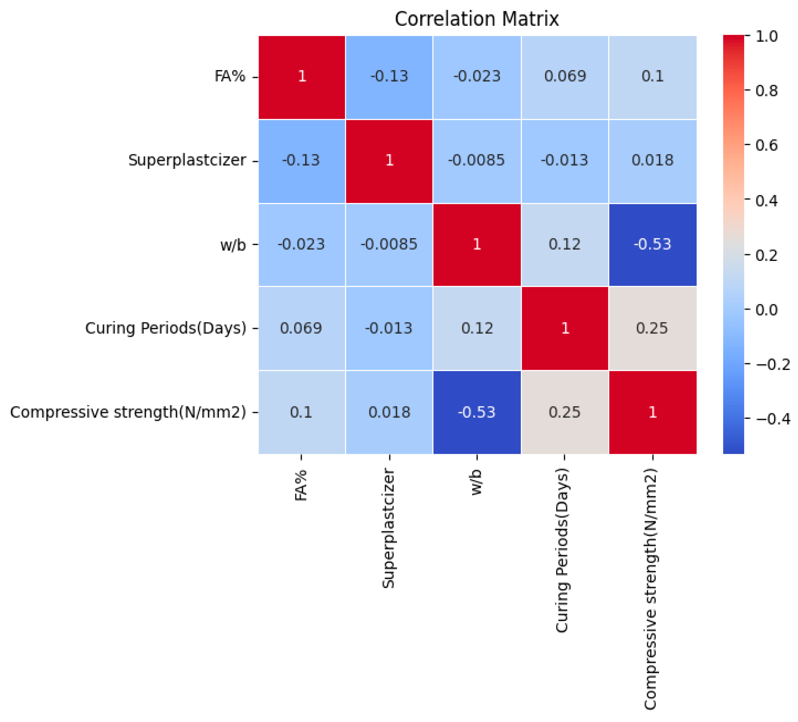
The relationships between variables are presented in the correlation matrix in Figure 3. A negative correlation is noted between the w/b and compressive strength. On the other hand, there is a positive correlation between the curing period and strength. A similar correlation is observed between FA percentage and superplasticizer content, but the relationship represented to the compressive strength in the correlation matrix is not significant. This means that a linear relationship between the FA percentage, superplasticizer content, and compressive strength cannot be guaranteed. These correlations assisted in understanding which variables have influence on the strength of UHPC, which resulted in comprehending the results of the best model prediction.

2.3. Data Normalization

This research utilized data normalization methods to get the dataset ready for using machine learning models. Making sure that all features are treated fairly and on a scale is crucial in the normalization process. This is especially important for models that are sensitive to the magnitude of the features. An overview of the techniques used for normalization is provided in this section.

2.3.1. Unnormalized Techniques

The examination began with the dataset in its unnormalized format. This method allows for the establishment of a starting point for evaluating the model’s performance using the data, which accurately represents the range of values. It also serves as a reference scenario, for comparing the effectiveness of normalization techniques. In this state, the data maintains its scale without any alterations made to the variable range.

2.3.2. Min-Max Normalization

Min-max normalization is a technique that rescales the feature to a fixed range of [0, 1]. It is calculated by subtracting the minimum value of the feature and then dividing by the range of the feature. Mathematically, for a value of x, the min-max normalized x ^ is given by Equation (1). This technique transformed all numeric inputs to a common scale without distorting differences in the ranges of values or losing information.
x ^ = x m i n ( x ) m a x ( x ) m i n ( x )

2.3.3. Z-Score Normalization

Also known as standardization, it involves rescaling the data to have a mean of 0 and a standard deviation of 1. The standardized value of x ( z ) for a given data point (x) is computed by subtracting the mean of the data ( μ ) from each data point and dividing the result by the standard deviation of the data ( σ ) as illustrated in Equation (2). This method of normalization is particularly useful when the data has a Gaussian (normal) distribution and when the algorithm assumes normally distributed data, such as Linear Regression and Support Vector Machines.
z = x μ σ

2.4. Machine Learning Techniques

2.4.1. Linear Regression

Linear regression is a technique in the field of machine learning that provides a straightforward approach to model the relationship between a dependent variable and one or more independent variables. It assumes a connection between the input variables (features) and the single output variable. The main principle behind regression is to adjust the weights of the input variables in order to minimize the discrepancy between predicted and actual output values, often using a least squares method. This optimization process serves as a step for other machine learning algorithms, making linear regression an essential starting point to comprehend more intricate models in this field [44]. The simplicity, interpretability, and ease of implementation associated with linear regression render it an invaluable tool within the realm of machine learning techniques [45]. Taking the theoretical background of linear regression into consideration and how it assumes a connection between the input variables and output, it should not be assumed that this model will not provide the best accuracy because some variables have a negative correlation. A positive correlation means that both of the variables will increase together whereas a negative correlation means one will increase while the other decreases. The key factor is whether the model captures the underlying relationship between the variables and target regardless of whether the relationship is positive or negative.

2.4.2. Support Vector Machine (SVM)

The Support Vector Machine (SVM) variant represents a significant advancement in the realm of machine learning algorithms. Linear SVM is known for its ability to classify data points by finding the separating hyperplane. It performs well in scenarios with dimensional data and often outperforms other algorithms in terms of accuracy and efficiency [45]. This algorithm achieves this by maximizing the margin between data points of classes which enhances its generalization abilities. Linear SVM is particularly effective in classification problems due to its capability to handle feature spaces and robustness against overfitting [46]. Additionally, by incorporating kernel tricks, SVMs can effectively handle real world applications where nonlinearly separable data is present [47]. The simplicity, efficiency, and versatility of linear SVM make it an essential tool for machine learning practitioners and researchers.
Polynomial SVM stands out among the machine learning algorithms due to its approach in handling complex relationships between data points that are not linear in nature. In contrast to its counterpart, the polynomial SVM makes use of kernel functions (polynomial kernels). These kernels help in projecting data into a space making it easier to separate data points that cannot be separated linearly in the original space [47]. The ability of the SVM to operate in transformed feature spaces allows it to handle a range of classification problems with more flexibility. The degree of the kernel plays a role as a hyperparameter. It determines the complexity of the decision boundary, which enables tuning for optimal performance on specific datasets [48]. One remarkable strength of the SVM is its capability to model patterns without significantly increasing computational burden. This is particularly useful when traditional linear models are not sufficient [49]. This balance between efficiency and modeling power makes the polynomial SVM an impressive tool for scenarios where complex data relationships are prevalent.
The Radial Basis Function (RBF) kernel used in Support Vector Machine (SVM) learning represents an advancement in handling linear problems, within machine learning. The RBF kernel possesses a Gaussian characteristic, which transforms the feature space into a dimension. This transformation enables the data that is not separable in a linear manner to be separated effectively. Researchers have found this technique to be highly effective in many applications [50]. One of the strengths of the RBF SVM lies in its ability to handle dimensional datasets using a relatively simple mathematical formulation. This approach maintains efficiency [51]. The selection of the kernel parameter, gamma, is an aspect of RBF SVM as it determines the curvature of the decision boundary. The flexibility it offers allows for tuning to achieve class separation even with intricate datasets [52]. Due to its proficiency in managing overfitting and robustness in spaces, the RBF SVM is a powerful tool for precision-oriented pattern recognition and classification tasks.
The SVM models provide advantages that can help in predicting the compressive strength of UHPC. Applying the right model is not easy but the SVM models have proven to be good at capturing the trends and behaviour of nonlinear variables. Some of the advantages, as mentioned above, are effectiveness in high dimensional space, kernel trick, and robustness to overfitting, which can be handy with variables like fly ash percentage, superplasticizer, and water-binder ratio. On the other hand, the reason why the SVM models are not necessarily the best for the dataset can be due to the model interpretability. SVM models might be more difficult to interpret compared to more transparent models like decision trees. This can be a drawback when the goal is to understand how different variables influence concrete strength. Moreover, there is a difficulty in dealing with multivariate regression because SVM is designed for classification tasks. While there are methods to adapt SVM for regression (e.g., SVR), these adaptations might not handle multivariate outputs as naturally as some other regression models, potentially complicating the prediction of concrete strength.

2.4.3. Random Forest

Random Forest is a robust ensemble learning technique used in machine learning. It builds upon the simplicity and effectiveness of decision trees. Random Forest works by creating decision trees during training and then determining the average prediction for regression from these individual trees. Random forests address the tendency of decision trees to overfit their training data by introducing randomness in two ways: by selecting a subset of the training data for building each tree (bootstrap sampling) and by considering only a random subset of features at each split within the trees. This method not only enhances the model’s accuracy, but it also presents the feature importance, which is crucial for understanding the underlying data patterns. Originally developed by Leo Breiman and Adele Cutler, Random Forest is highly regarded for its simplicity, user friendliness, and adaptability, making it suitable for tasks such as classification and regression without requiring hyperparameter tuning in many scenarios. Its resistance to overfitting and its capability to handle datasets with dimensionality have established it as a fundamental algorithm in the toolset of numerous data scientists and machine learning professionals [53]. When utilizing Random Forest to estimate the strength of UHPC, it proves beneficial due to its ability to comprehensively assess relationships among elements such as FA%, superplasticizers, and curing period. Moreover, its collaborative approach mitigates overfitting issues as mentioned before, thereby improving its precision when dealing with data through the combined power of multiple decision trees.

2.4.4. Artificial Neural Networks (ANN)

Artificial Neural Networks (ANN) are inspired by biological neural networks found in animal brains. Neural networks consist of interconnected nodes arranged in layers that neurons structure within our brain. These nodes collectively perform tasks. This framework allows them to represent nonlinear relationships in data, which proves highly effective in tasks such as recognizing images and speech as pointed out by [54]. The flexibility and adaptability of networks emerge from their ability to learn and adjust these connections through a process called backpropagation as described by [55]. This process enables the weights to be modified based on the difference between predicted and actual outcomes, continuously enhancing the accuracy of the model. The emergence of learning a branch of machine learning that focuses on networks with multiple layers (known as deep neural networks) has further broadened their capabilities. It allows for extracting high level features from data as explained by [56]. Neural networks are a great fit for forecasting the strength of UHPC as they can handle connections among factors such as FA%, superplasticizer, and curing period. Their deep learning skills allow them to grasp details from datasets capturing patterns and the nonlinear relationships that enhance prediction accuracy significantly.

2.5. Model Performance Evaluation

During the evaluation phase of the ML models, two measurement metrics were used to assess the performance and accuracy. One of them is R squared ( R 2 ), also known as the coefficient of determination, and the other root mean squared error (RMSE). Both R 2 and RMSE played crucial roles in the methodology to ensure an accurate evaluation of the models’ predictive power. The metrics are further explained with the equations below. R 2 was used as a metric that informs how well the model replicates the outcomes by measuring the proportion of total outcome variation explained by the model [57]. It essentially shows how well the model fits the data. In the R 2 equation (Equation (5)), the sum of residual squares ( S S r e s ) and the total sum of squares ( S S t o t ) are evaluated to calculate the R 2 values. As mentioned before, a higher R 2 value, which can be quantified by it being closer to one, indicates that the ML model explains a large portion of the variance in the target variable, suggesting a good fit to the data. On the other hand, MSE quantifies the squared difference between the observed actual outcomes and those predicted by the model. It directly reflects how much error there is on average, making it an important metric for assessing a model’s accuracy. In the RMSE equation (Equation (6)), n is the number of observations in the dataset. The other two important variables are y i and y ^ i which are the actual value of the i-th observation and the predicted value for the i-th observation, respectively. A lower MSE (closer to zero) suggests a good model in terms of its predictive ability.
S S r e s = i = 1 n ( y i y ^ i ) 2
S S t o t = i = 1 n ( y i ȳ ) 2
R 2 = 1 S S r e s S S t o t  
R M S E = 1 n i = 1 n ( y i y ^ i ) 2

3. Results and Discussion

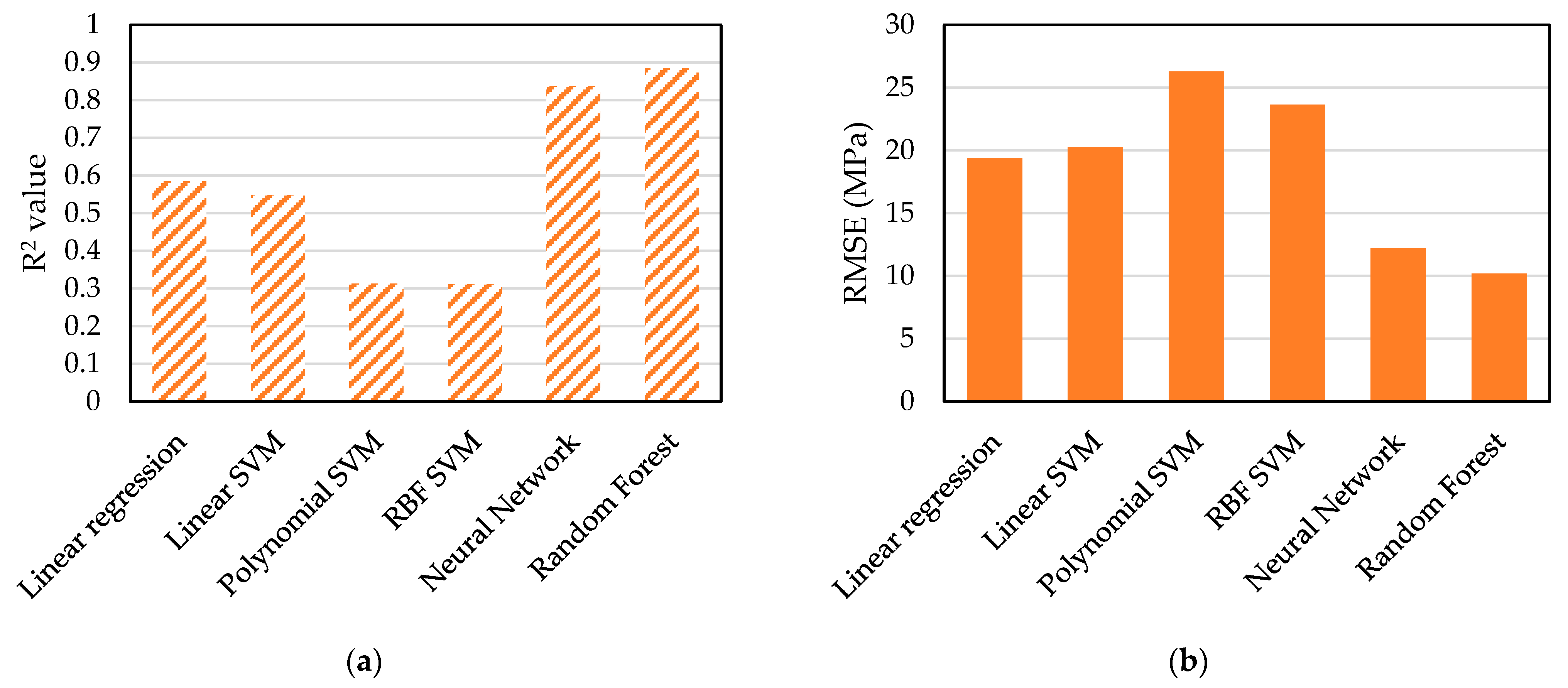
The study focused on predicting the compressive strength of UHPC with different FA replacement percentages, superplasticizer content, w/b, and curing period. The accuracy of each model was assessed using R2 and RMSE values. The analysis presented in Figure 4 evaluated models to predict the compressive strength of UHPC. The first bar represents Linear Regression, which showed moderate prediction accuracy across initial states. The second and third bars illustrate the performance of Linear SVM and Polynomial SVM models, respectively. The range of R2 values displayed by these models indicates varying levels of prediction accuracy. The fourth bar represents the RBF SVM model that performed well under one initial condition, suggesting its potential for high performance based on how the data is divided. The fifth bar corresponds to the ANN model which consistently demonstrated a high R2 values across all states, highlighting its ability to decipher complex patterns in UHPC’s compressive strength data. The last bar represents the results of Random Forest, which demonstrated the highest accuracy out of all the machine learning models used on the dataset. As mentioned previously, the RMSE is a measure of the differences between values predicted by a model and the values actually observed, with lower RMSE values indicating better fit. In a similar manner, Random Forest model outperforms all others with the lowest RMSE, indicating that it has the best predictive accuracy and the smallest average error in the prediction of UHPC’s compressive strength. This method, which involves creating decision trees and combining their predictions, showed capability in capturing intricate data relationships. Its success can be attributed to its feature selection process and the use of randomness to prevent overfitting in each tree data subset. This accomplishment underscores the versatility and effectiveness of the Random Forest technique across datasets and modelling scenarios, establishing it as a tool in predictive analytics. The Neural Network also performed relatively well compared to other ML models, achieving a R2 score of 0.8421.
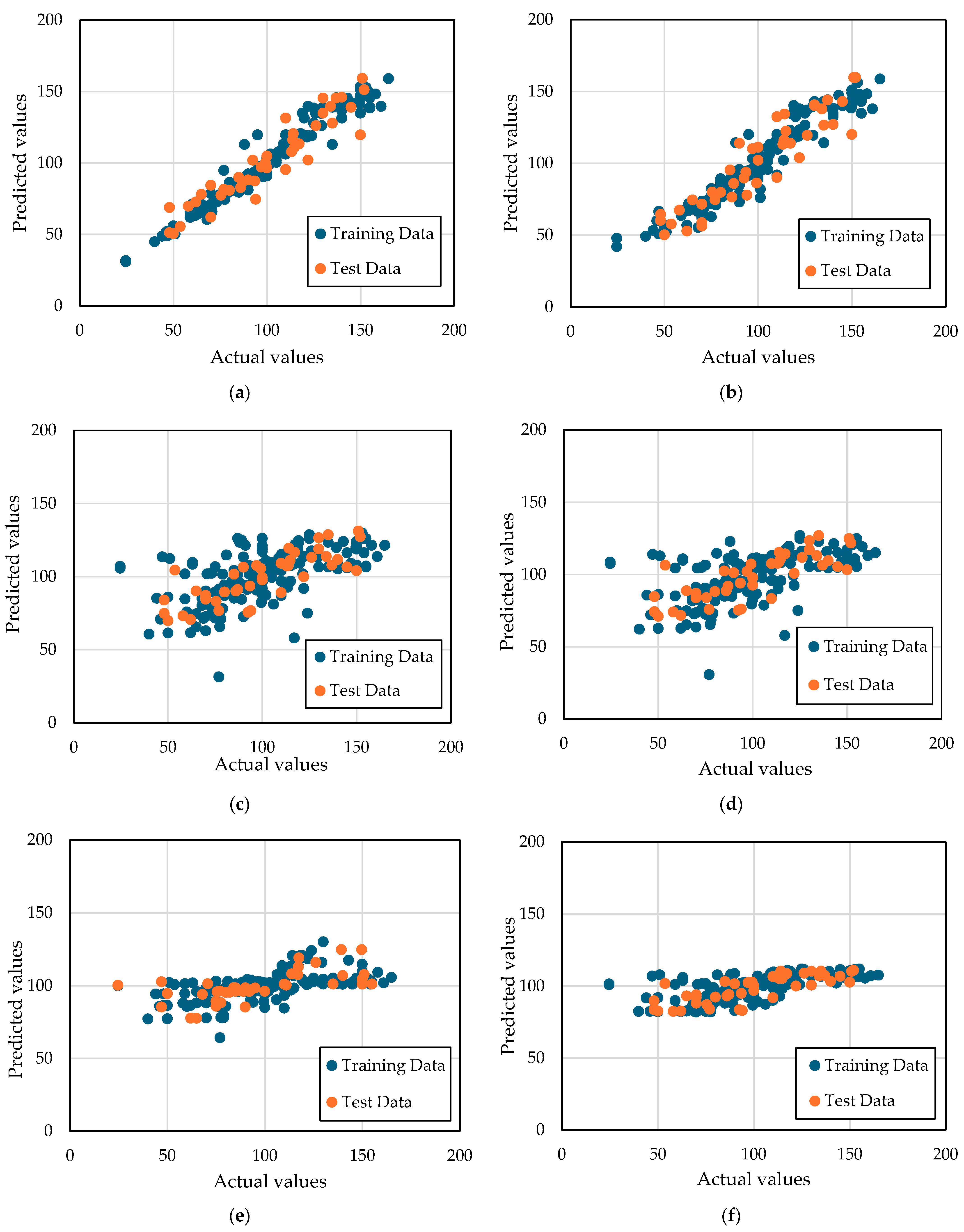
The predicted versus actual values are presented for each ML model in Figure 5. It can be observed that Figure 5a,b that correspond to Random Forest and ANN, respectively, demonstrate the best fit (data points are close to the unity line). The data points align closely along the line of agreement indicating that the predictions of both models are highly accurate. It is worth noting that the scatter plot shows a pattern in the model’s predictions for values in the mid to high range, suggesting that it effectively captures the underlying patterns within this specific part of the dataset.
Linear Regression achieved a satisfactory level of predictive ability with an R2 score of 0.5844 suggesting it could capture some variations in UHPC strength. However, there is a gap between its performance and that of the Random Forest and Neural Network, which highlights Linear Regression’s limitations in comprehending the complexity of the data. This discrepancy is likely due to Linear Regression’s nature, which restricts its ability to accurately represent linear relationships and interactions necessary for predicting UHPC’s strength as presented by Figure 5c. It is clear from the graph that there is a trend but also some variation around the line of perfect prediction, especially as the actual values get higher. This suggests that while the Linear Regression model captures the trend, it may not consider all the factors that contribute to variability in the data. As a result, its predictions become less accurate for levels of strength.
The SVM models demonstrated varying degrees of accuracy, all lower than both Random Forest and Neural Network. The Linear SVM model, with an R2 score of 0.5473 did a satisfactory job in predicting UHPC’s strength too. It seems that the linear decision boundaries imposed by the Linear SVM could not capture the relationships within the dataset properly. This highlights the challenges of using linear models for regression tasks. Similarly, the Polynomial SVM model had a predictive accuracy with an R2 score of 0.3124. Despite introducing nonlinearity through kernels, this model struggled to represent the complexity of the data. The difficulty in selecting a degree and kernel parameters might have contributed to its less-than-optimal performance showing how sensitive SVM models can be to these tuning parameters. Moreover, the RBF SVM model has an R2 score of 0.3836. Even though the RBF kernel can capture linear relationships by mapping input features into a higher dimensional space, it was not enough to effectively represent the complexity of our dataset. This emphasizes how important it is to tune RBF SVM parameters and consider the computational intensity that can impact its performance if not handled properly. In Figure 5d–f, the results of the three SVM models that were used to predict the strength of UHPC are presented. Each model utilized a different normalization technique. Figure 5d shows the performance of the Linear SVM model, with Z-Score normalization. It demonstrates a linear relationship between the predicted values indicating a strong fit for the model. However, there is some variability in the predicted values, suggesting that the model’s precision may vary. Figure 5e shows the Polynomial SVM model with Min-Max normalization. It also exhibits a trend with greater dispersion, indicating that it might be more sensitive to the nonlinear nature of the data. Finally, Figure 5f showcases the RBF SVM model with Z-Score normalization. The predictions cluster closer along the unity line than the two other models, suggesting that this model captures linear relationships in the dataset more effectively.

4. Parametric Study

The best prediction model in Section 3 –Random Forest– was used for a parametric study, in which the parameters affecting the compressive shear strength of UHPC mix can be varied and their effect can be studied. In this investigation, a parametric analysis was carried out on the influence of different FA replacement percentages and superplasticizer dosages at different curing periods.
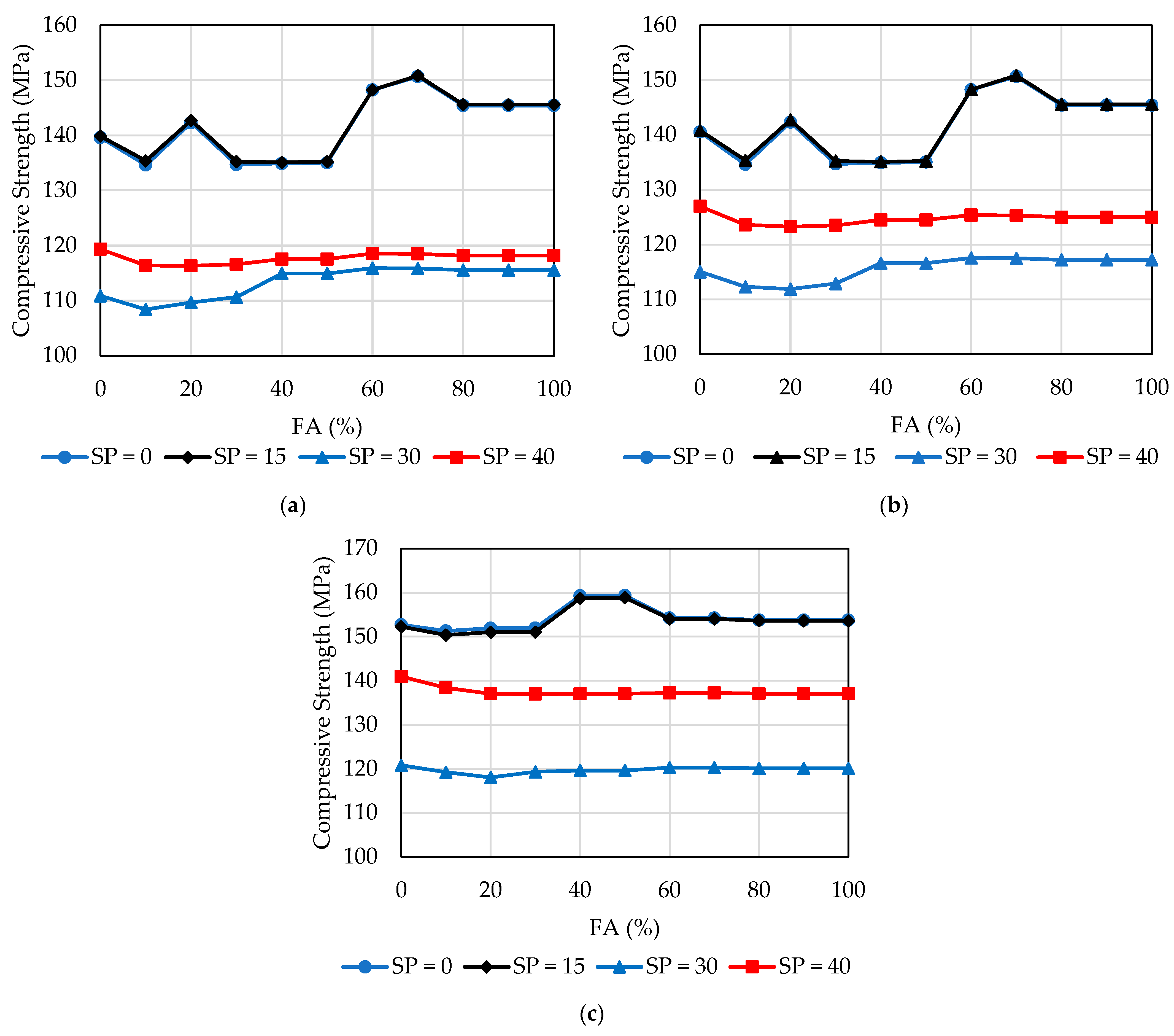
The parametric study was carried out by varying the FA replacement percentages from 0 to 100%, at four dosages of superplasticizer (0, 15, 30, 40), both at three curing periods (28, 56, and 120 days), respectively. The main aim of the study is to investigate the effect of higher FA replacement percentages (>60%) at longer curing periods. The study was conducted by setting the w/b ratio to 0.15, which is most common w/b ratio used in UHPC mixes. Another reason for fixing the w/b ratio is because it has a negative correlation to the compressive strength, so decreasing it to the most minimal possible value will give the best results. Figure 6 demonstrates the results using the most accurate Random Forest model. It can be detected from the Figure 6a that the maximum compressive strength values obtained were at superplasticizer levels of 0 and 15, where they all had 150 MPa strength. The superplasticizer levels of 30 and 40 had a compressive strength value of 115 and 118, respectively. All those values were found to be at a FA% of 70. The results in Figure 6b, where the curing days are 56, are very similar to the results found in Figure 6a, with a curing time of 28 days. Similarly, the maximum compressive strength is at the superplasticizer levels of 0 and 15, where the strength is 150 MPa. The other superplasticizer levels (30 and 40) have a compressive strength of 117 and 125, respectively, which are slightly higher than the ones found in Figure 6a at the same levels.
Lastly, the final findings of the parametric tests were conducted by varying the curing period to 120 days as shown in Figure 6c. The results in the figure show a significant increase in the compressive strength of the UHPC mix with a fly ash percentage of 50 at superplasticizer levels 0 and 15, respectively. The compressive strength on average increased by 24 MPa when comparing it to the results at 56 curing days. This finding in the parametric study provided the highest compressive strength result of 159 MPa. As accurate as the Random Forest model was, those results were not exactly expected. The few previous conducted experiments in the literature showed an even higher increase in the compressive strength when comparing 28 to 120 days. The mix that had the highest compressive strength at 28 days only increased by 4 MPa at 120 days while taking into consideration the fly ash percentage was 70%. Whereas the mix that had the highest compressive strength at 120 days increased by 24 MPa when comparing it to its strength at 28 days as mentioned above. Additionally, the results are lining up correctly with the facts previously stated about how fly ash percentage affects the compressive strength of UHPC. This could be proven correct in this parametric study when comparing the compressive strength of a mix with the following parameters of a fly ash percentage at 100 and superplasticizer at 0. This specific mix increased its compressive strength by 8 MPa when going from 28 to 120 days. This shows that the model is able to capture the trends in the mix design and accurately predict the strength even though some of the parameters have a nonlinear relationship. This parametric study can be further enhanced by expanding the dataset to have more points of compressive strength UHPC mix results with 120 days and above.

5. Conclusions

This study utilized previously published data on the compressive strength of UHPC with different FA replacement percentages to create a predictive model of the UHPC’s compressive strength using six ML models. The model also takes into consideration other parameters, including w/b ratio, superplasticizer content, and curing period. After choosing the best prediction model using comparative performance measures, the model was used to predict the UHPC’s strength with various FA%. The following conclusions can be drawn out of the study:
  • The Random Forest ML model emerged as the top performer in predicting UHPC’s strength with an R2 value of 0.8857. This was achieved due to the Random Forest model being able to capture complex nonlinear relationships inherent in the dataset. The results achieved with the model emphasize the value of leveraging advanced algorithms that can handle multidimensional data and interaction effects more effectively than simple traditional models.
  • Traditional modelling techniques such as Linear Regression and SVMs showed limited capability in accurately predicting UHPC strength where the best model out of them had an accuracy of 0.5844. This limitation points to the difficulties of applying linear or margin-based models to phenomena characterized by complex interactions and nonlinear dependencies. This highlights the importance of considering the relationship between the different variables before applying the models. Variables like w/b ratio and superplasticizer have a complex relationship with UHPC’s strength that cannot be captured with a simple traditional model like linear regression.
  • The research emphasizes the necessity of broadening the scope of data collection to include a wider array of conditions, processing parameters, and material compositions. The parametric study was performed but limited by the variety of data in the dataset. After 120 days the predictive model was not able to predict the increase in strength of the concrete.

Author Contributions

Conceptualization, R.A.H. and S.K.S.; methodology, H.S. and R.A.H.; software, H.S., R.A.H. and R.H.; validation, H.S., R.A.H., M.A. and J.A.; formal analysis, H.S. and R.H.; investigation, H.S. and M.A.; resources, R.A.H., J.A. and S.K.S.; data curation, S.K.S.; writing—original draft preparation, H.S., M.A. and S.K.S.; writing—review and editing, M.A. and R.A.H.; visualization, H.S. and M.A.; supervision, M.A., R.A.H. and J.A.; project administration, R.A.H. and J.A.; funding acquisition, R.A.H. All authors have read and agreed to the published version of the manuscript.

Funding

This research received no external funding.

Data Availability Statement

The data that support the findings of this study are available from the corresponding author, R.A.H., upon reasonable request.

Acknowledgments

This research was funded by American University of Sharjah and Riad T. Sadek Endowed Chair in Civil Engineering. The support is gratefully acknowledged and appreciated.

Conflicts of Interest

The authors declare no conflicts of interest.

Appendix A

Table A1. Collected data.
ReferenceFA (%)Superplasticizer (kg/m3)w/bCuring Period (Days)Compressive Strength (MPa)
Ferdosian et al. [19]000.228150
1000.228140
1500.228145
2000.228155
2500.228137
3000.228137
3500.228140
2000.228145
2000.228145
2500.228155
3000.228150
Chen et al. [20]030.20.2159
030.20.2795.7
030.20.228106.3
030.20.256108.8
030.20.290114.1
030.20.2170.7
030.20.2797.4
030.20.228113.2
030.20.256113.8
030.20.290118.1
2030.20.2153.7
2030.20.2799.2
2030.20.228109.9
2030.20.256110.3
2030.20.290117.5
3030.20.2124.6
3030.20.27101.2
3030.20.228114.8
3030.20.256117.2
3030.20.290119.3
4030.20.2124.6
4030.20.27101.2
4030.20.228114.8
4030.20.256117.2
4030.20.290119.3
034.20.2172.8
034.20.27102.8
034.20.228113.8
034.20.256126.2
034.20.290139.3
034.20.2172.8
034.20.27102.8
034.20.228113.8
034.20.256126.2
034.20.290139.3
034.20.2173.2
034.20.27102.3
034.20.228115.2
034.20.256129.3
034.20.290149.7
Alsalman et al. [22]05.110.4340
05.110.4750
05.110.42865
05.110.45678
05.110.49179
05.110.421079
304.770.3348
304.770.3759
304.770.32875
304.770.35685
304.770.39187
304.770.321089
404.750.3344
404.750.3750
404.750.32865
404.750.35688
404.750.39186
404.750.321087
06.770.3368
06.770.3771
06.770.32885
06.770.35697
06.770.391100
06.770.3210100
404.240.3368
404.240.3770
404.240.32886
404.240.35697
404.240.391100
404.240.3210100
Hakeem et al. [37]000.1528161
4000.1528150
6000.1528158
8000.1528143
10000.1528130
Haque & Kayali [43]060.4762
060.41470
060.42877.5
1060.35770
1060.351477.5
1060.352894
1060.355699.5
1560.35758
1560.351465
1560.352873.5
07.50.35769
07.50.351475
07.50.352892.5
07.50.3556106
107.50.25784
107.50.251493.5
107.50.2528111
107.50.2556121.5
157.50.3775.5
157.50.31489
157.50.328102
157.50.356113.5
Hasnat & Ghafoori [38]000.15163
000.157105
000.1528134
000.1590153
1000.15163
1000.157102
1000.1528129
1000.1590152
3000.15151
3000.15790
3000.1528126
3000.1590153
4000.15147
4000.15781
4000.1528119
4000.1590151
Wang et al. [39]000.12888
000.1228135
000.1528122
000.1828110
000.22895
000.232888
000.252880
000.32870
2000.128125
2000.1228155
2000.1528145
2000.1828135
2000.228130
2000.2328115
2000.2528110
2000.328110
4000.128125
4000.1228135
4000.1528130
4000.1828120
4000.228110
4000.2328105
4000.2528100
4000.328100
000.35350
000.35762
000.352848
000.359080
800.35346
800.35775
800.352860
800.3590100
1500.35347
1500.35790
1500.352877
1500.3590110
000.25375
000.25770
000.252890
000.259090
800.25385
800.25787
800.252895
800.259097
1500.25392
1500.257100
1500.2528100
1500.2590100
Wu et al. [40]000.2398
000.27122
000.228150
000.290154
2000.2385
2000.27105
2000.228135
2000.290150
4000.2385
4000.27105
4000.228140
4000.290165
6000.2375
6000.2793
6000.228140
6000.290150
Yazici [41]0450.228117
20450.328122
40450.428124
60450.528117
80450.652877
Jaturapitakkul et al. [42]1560.3770
1560.32880
1560.35690
1560.39095
1560.3180100
255.30.3770
255.30.32882
255.30.35692
255.30.39095
255.30.3180100
354.30.3770
354.30.32880
354.30.35688
354.30.39093
354.30.3180100
503.20.3770
503.20.32877
503.20.35684
503.20.39087
503.20.318091

References

  1. Wu, Z.; Shi, C.; He, W.; Wang, D. Uniaxial Compression Behavior of Ultra-High Performance Concrete with Hybrid Steel Fiber. J. Mater. Civ. Eng. 2016, 28, 06016017. [Google Scholar] [CrossRef]
  2. Habel, K.; Viviani, M.; Denarié, E.; Brühwiler, E. Development of the mechanical properties of an Ultra-High Performance Fiber Reinforced Concrete (UHPFRC). Cem. Concr. Res. 2006, 36, 1362–1370. [Google Scholar] [CrossRef]
  3. Park, S.H.; Kim, D.J.; Ryu, G.S.; Koh, K.T. Tensile behavior of Ultra High Performance Hybrid Fiber Reinforced Concrete. Cem. Concr. Compos. 2012, 34, 172–184. [Google Scholar] [CrossRef]
  4. Shi, C.; Wu, Z.; Xiao, J.; Wang, D.; Huang, Z.; Fang, Z. A review on ultra high performance concrete: Part I. Raw materials and mixture design. Constr. Build. Mater. 2015, 101, 741–751. [Google Scholar] [CrossRef]
  5. Kim, H.; Moon, B.; Hu, X.; Lee, H.; Ryu, G.S.; Koh, K.T.; Joh, C.; Kim, B.S.; Keierleber, B. Construction and performance monitoring of innovative ultra-high-performance concrete bridge. Infrastructures 2021, 6, 121. [Google Scholar] [CrossRef]
  6. Ali, B.; Farooq, M.A.; El Ouni, M.H.; Azab, M.; Elhag, A.B. The combined effect of coir and superplasticizer on the fresh, mechanical, and long-term durability properties of recycled aggregate concrete. J. Build. Eng. 2022, 59, 105009. [Google Scholar] [CrossRef]
  7. Arshad, S.; Sharif, M.B.; Irfan-Ul-Hassan, M.; Khan, M.; Zhang, J.-L. Efficiency of Supplementary Cementitious Materials and Natural Fiber on Mechanical Performance of Concrete. Arab. J. Sci. Eng. 2020, 45, 8577–8589. [Google Scholar] [CrossRef]
  8. Abdalla, J.A.; Hawileh, R.A.; Bahurudeen, A.; Jyothsna, G.; Sofi, A.; Shanmugam, V.; Thomas, B. A comprehensive review on the use of natural fibers in cement/geopolymer concrete: A step towards sustainability. Case Stud. Constr. Mater. 2023, 19, e02244. [Google Scholar] [CrossRef]
  9. RHawileh, R.A.; Mhanna, H.H.; Abdalla, J.A.; AlMomani, D.; Esrep, D.; Obeidat, O.; Ozturk, M. Properties of concrete replaced with different percentages of recycled aggregates. Mater. Today Proc. 2023. [Google Scholar] [CrossRef]
  10. Mantawy, I.; Chennareddy, R.; Genedy, M.; Taha, M.R. Polymer Concrete for Bridge Deck Closure Joints in Accelerated Bridge Construction. Infrastructures 2019, 4, 31. [Google Scholar] [CrossRef]
  11. Kurniati, E.O.; Kim, H.-J. Utilizing Industrial By-Products for Sustainable Three-Dimensional-Printed Infrastructure Applications: A Comprehensive Review. Infrastructures 2023, 8, 140. [Google Scholar] [CrossRef]
  12. Eisa, A.S.; Sabol, P.; Khamis, K.M.; Attia, A.A. Experimental Study on the Structural Response of Reinforced Fly Ash-Based Geopolymer Concrete Members. Infrastructures 2022, 7, 170. [Google Scholar] [CrossRef]
  13. Hawileh, R.A.; Quadri, S.S.; Abdalla, J.A.; Assad, M.; Thomas, B.S.; Craig, D.; Naser, M.Z. Residual mechanical properties of recycled aggregate concrete at elevated temperatures. Fire Mater. 2023, 48, 138–151. [Google Scholar] [CrossRef]
  14. Abdalla, J.A.; Hawileh, R.A.; Tariq, R.; Abdelkhalek, M.; Abbas, S.; Khartabil, A.; Khalil, H.T.; Thomas, B.S. Achieving concrete sustainability using crumb rubber and GGBS. Mater. Today Proc. 2023. [Google Scholar] [CrossRef]
  15. Hawileh, R.A.; Abdalla, J.A.; Nawaz, W.; Zadeh, A.S.; Mirghani, A.; Al Nassara, A.; Khartabil, A.; Shantia, M. Effects of Replacing Cement with GGBS and Fly Ash on the Flexural and Shear Performance of Reinforced Concrete Beams. Pr. Period. Struct. Des. Constr. 2024, 29, 04024011. [Google Scholar] [CrossRef]
  16. Tariq, H.; Siddique, R.M.A.; Shah, S.A.R.; Azab, M.; Rehman, A.U.; Qadeer, R.; Ullah, M.K.; Iqbal, F. Mechanical Performance of Polymeric ARGF-Based Fly Ash-Concrete Composites: A Study for Eco-Friendly Circular Economy Application. Polymers 2022, 14, 1774. [Google Scholar] [CrossRef] [PubMed]
  17. Jiang, X.; Xiao, R.; Zhang, M.; Hu, W.; Bai, Y.; Huang, B. A laboratory investigation of steel to fly ash-based geopolymer paste bonding behavior after exposure to elevated temperatures. Constr. Build. Mater. 2020, 254, 119267. [Google Scholar] [CrossRef]
  18. Khan, M.; Ali, M. Improvement in concrete behavior with fly ash, silica-fume and coconut fibres. Constr. Build. Mater. 2019, 203, 174–187. [Google Scholar] [CrossRef]
  19. Ferdosian, I.; Camões, A.; Ribeiro, M. High-volume fly ash paste for developing ultra-high performance concrete (UHPC). Cienc. Tecnol. Dos Mater. 2017, 29, e157–e161. [Google Scholar] [CrossRef]
  20. JChen, J.; Ng, P.; Li, L.; Kwan, A. Production of High-performance Concrete by Addition of Fly Ash Microsphere and Condensed Silica Fume. Procedia Eng. 2017, 172, 165–171. [Google Scholar] [CrossRef]
  21. Nath, P.; Sarker, P. Effect of Fly Ash on the Durability Properties of High Strength Concrete. Procedia Eng. 2011, 14, 1149–1156. [Google Scholar] [CrossRef]
  22. Alsalman, A.; Dang, C.N.; Hale, W.M. Development of ultra-high performance concrete with locally available materials. Constr. Build. Mater. 2017, 133, 135–145. [Google Scholar] [CrossRef]
  23. Gong, N.; Zhang, N. Predict the compressive strength of ultra high-performance concrete by a hybrid method of machine learning. J. Eng. Appl. Sci. 2023, 70, 107. [Google Scholar] [CrossRef]
  24. Hu, X.; Shentu, J.; Xie, N.; Huang, Y.; Lei, G.; Hu, H.; Guo, P.; Gong, X. Predicting triaxial compressive strength of high-temperature treated rock using machine learning techniques. J. Rock Mech. Geotech. Eng. 2023, 15, 2072–2082. [Google Scholar] [CrossRef]
  25. Zhang, Y.; An, S.; Liu, H. Employing the optimization algorithms with machine learning framework to estimate the compressive strength of ultra-high-performance concrete (UHPC). Multiscale Multidiscip. Model. Exp. Des. 2024, 7, 97–108. [Google Scholar] [CrossRef]
  26. Qian, Y.; Sufian, M.; Accouche, O.; Azab, M. Advanced machine learning algorithms to evaluate the effects of the raw ingredients on flowability and compressive strength of ultra-high-performance concrete. PLoS ONE 2022, 17, e0278161. [Google Scholar] [CrossRef] [PubMed]
  27. Shen, Z.; Deifalla, A.F.; Kamiński, P.; Dyczko, A. Compressive Strength Evaluation of Ultra-High-Strength Concrete by Machine Learning. Materials 2022, 15, 3523. [Google Scholar] [CrossRef] [PubMed]
  28. Abuodeh, O.R.; Abdalla, J.A.; Hawileh, R.A. Assessment of compressive strength of Ultra-high Performance Concrete using deep machine learning techniques. Appl. Soft Comput. 2020, 95, 106552. [Google Scholar] [CrossRef]
  29. Khan, M.; Lao, J.; Dai, J.-G. Comparative study of advanced computational techniques for estimating the compressive strength of UHPC. J. Asian Concr. Fed. 2022, 8, 51–68. [Google Scholar] [CrossRef]
  30. Yuan, Y.; Yang, M.; Shang, X.; Xiong, Y.; Zhang, Y. Predicting the Compressive Strength of UHPC with Coarse Aggregates in the Context of Machine Learning. Case Stud. Constr. Mater. 2023, 19, e02627. [Google Scholar] [CrossRef]
  31. Marani, A.; Jamali, A.; Nehdi, M.L. Predicting Ultra-High-Performance Concrete Compressive Strength Using Tabular Generative Adversarial Networks. Materials 2020, 13, 4757. [Google Scholar] [CrossRef] [PubMed]
  32. Lu, J.; Yu, Z.; Zhu, Y.; Huang, S.; Luo, Q.; Zhang, S. Effect of Lithium-Slag in the Performance of Slag Cement Mortar Based on Least-Squares Support Vector Machine Prediction. Materials 2019, 12, 1652. [Google Scholar] [CrossRef] [PubMed]
  33. Solhmirzaei, R.; Salehi, H.; Kodur, V.; Naser, M.Z. Machine learning framework for predicting failure mode and shear capacity of ultra high performance concrete beams. Eng. Struct. 2020, 224, 111221. [Google Scholar] [CrossRef]
  34. Abellan-Garcia, J. Four-layer perceptron approach for strength prediction of UHPC. Constr. Build. Mater. 2020, 256, 119465. [Google Scholar] [CrossRef]
  35. Fan, D.; Yu, R.; Fu, S.; Yue, L.; Wu, C.; Shui, Z.; Liu, K.; Song, Q.; Sun, M.; Jiang, C. Precise design and characteristics prediction of Ultra-High Performance Concrete (UHPC) based on artificial intelligence techniques. Cem. Concr. Compos. 2021, 122, 104171. [Google Scholar] [CrossRef]
  36. Serna, P.; Llano-Torre, A.; Martí-Vargas, J.R.; Navarro-Gregori, J. (Eds.) Fibre Reinforced Concrete: Improvements and Innovations RILEM-fib International Symposium on FRC (BEFIB) in 2020; RILEM Bookseries; Springer: Berlin/Heidelberg, Germany, 2021; Available online: http://www.springer.com/series/8781 (accessed on 5 January 2024).
  37. Hakeem, I.Y.; Althoey, F.; Hosen, A. Mechanical and durability performance of ultra-high-performance concrete incorporating SCMs. Constr. Build. Mater. 2022, 359, 129430. [Google Scholar] [CrossRef]
  38. Hasnat, A.; Ghafoori, N. Properties of ultra-high performance concrete using optimization of traditional aggregates and pozzolans. Constr. Build. Mater. 2021, 299, 123907. [Google Scholar] [CrossRef]
  39. Wang, Q.; Wang, D.; Chen, H. The role of fly ash microsphere in the microstructure and macroscopic properties of high-strength concrete. Cem. Concr. Compos. 2017, 83, 125–137. [Google Scholar] [CrossRef]
  40. Wu, Z.; Shi, C.; He, W. Comparative study on flexural properties of ultra-high performance concrete with supplementary cementitious materials under different curing regimes. Constr. Build. Mater. 2017, 136, 307–313. [Google Scholar] [CrossRef]
  41. Yazici, H. The effect of curing conditions on compressive strength of ultra high strength concrete with high volume mineral admixtures. Build. Environ. 2007, 42, 2083–2089. [Google Scholar] [CrossRef]
  42. Jaturapitakkul, C.; Kiattikomol, K.; Sata, V.; Leekeeratikul, T. Use of ground coarse fly ash as a replacement of condensed silica fume in producing high-strength concrete. Cem. Concr. Res 2004, 34, 549–555. [Google Scholar] [CrossRef]
  43. Haque, M.; Kayali, O. Properties of high-strength concrete using a fine fly ash. Cem. Concr. Res. 1998, 28, 1445–1452. [Google Scholar] [CrossRef]
  44. Christopher, M. Bishop, Pattern Recognition and Machine Learning; Springer: Berlin/Heidelberg, Germany, 2006. [Google Scholar]
  45. Hastie, T.; Tibshirani, R.; Friedman, J. The Elements of Statistical Learning; Springer: Berlin/Heidelberg, Germany, 2009. [Google Scholar]
  46. Boser, B.E.; Guyon, I.M.; Vapnik, V.N. A Training Algorithm for Optimal Margin Classifiers. In Proceedings of the Fifth Annual Workshop on Computational Learning Theory, Pittsburgh, PA, USA, 27–29 July 1992; pp. 144–152. [Google Scholar]
  47. Schölkopf, B.; Burges, C.J.; Smola, A.J. Advances in Kernel Methods: Support Vector Learning; MIT Press: Cambridge, MA, USA, 2002. [Google Scholar]
  48. Chin-Chung, C. LIBSVM: A Library for Support Vector Machines. ACM Trans. Intell. Syst. Technol. 2011, 2, 27. [Google Scholar]
  49. Hofmann, T.; Schölkopf, B.; Smola, A.J. Kernel Methods in Machine Learning. Ann. Stat. 2008, 36, 1171–1220. [Google Scholar] [CrossRef]
  50. Burges, C.J.C. A Tutorial on Support Vector Machines for Pattern Recognition. Data Min. Knowl. Discov. 1998, 2, 121–167. [Google Scholar] [CrossRef]
  51. Schölkopf, B. Kernel Principal Component Analysis. In Proceedings of the Artificial Neural Networks—ICANN’97, Lausanne, Switzerland, 8–10 October 1997; pp. 583–588. [Google Scholar]
  52. Hsu, C.W.; Chang, C.C.; Lin, C.J. A Practical Guide to Support Vector Classification. 2016. Available online: https://www.csie.ntu.edu.tw/~cjlin/ (accessed on 10 January 2024).
  53. Breiman, L. Random Forests. Mach. Learn. 2001, 45, 5–32. [Google Scholar] [CrossRef]
  54. LeCun, Y.; Bengio, Y.; Hinton, G. Deep Learning. Nature 2015, 521, 436–444. [Google Scholar] [CrossRef] [PubMed]
  55. Rumelhart, D.E.; Hinton, G.E.; Williams, R.J. Learning Representations by Back-Propagating Errors. Nature 1986, 323, 533–536. [Google Scholar] [CrossRef]
  56. Goodfellow, I.; Bengio, Y.; Courville, A. Deep Learning; MIT Press: Cambridge, MA, USA, 2016. [Google Scholar]
  57. James, G.; Witten, D.; Hastie, T.; Tibshirani, R. An Introduction to Statistical Learning; Springer: Berlin/Heidelberg, Germany, 2013. [Google Scholar]
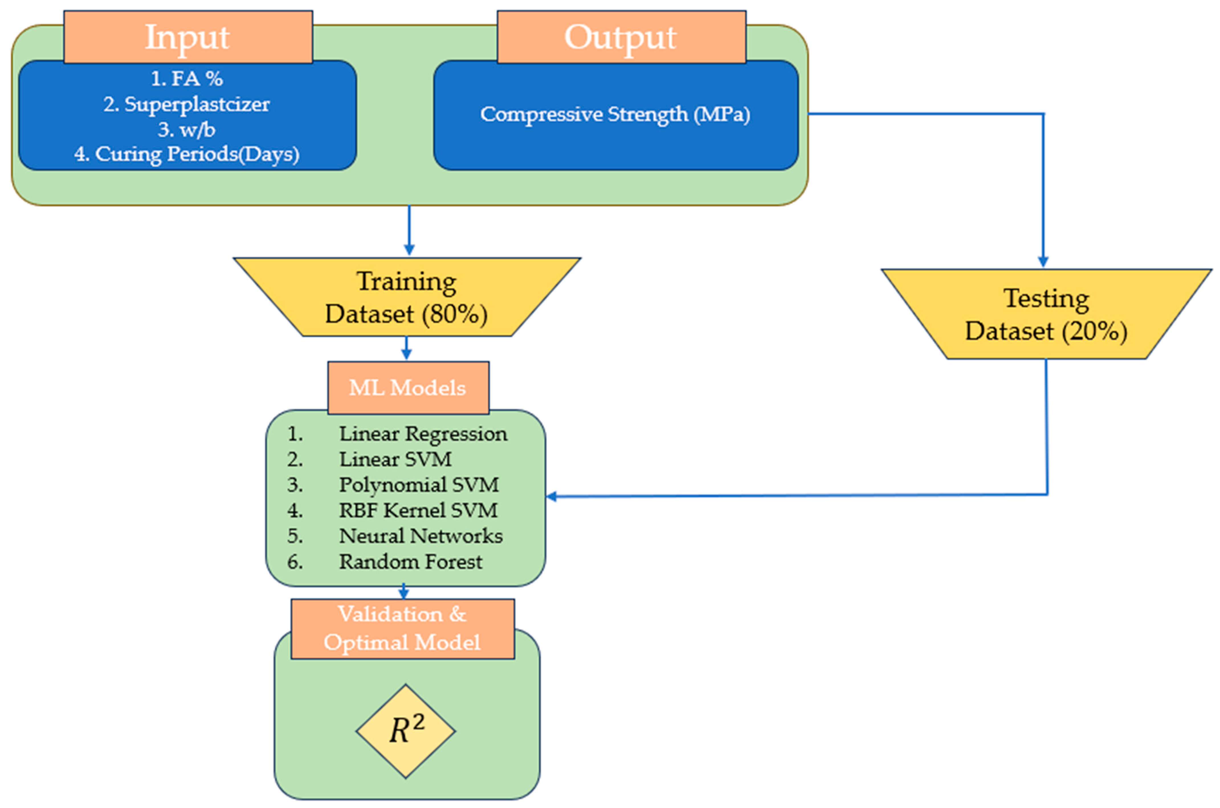
Figure 1. Methodology.
Infrastructures 09 00092 g001
Figure 2. Distribution of the collected data: (a) Fly ash percentage (FA%); (b) Superplasticizer content; (c) Water to binder ratio (w/b); (d) Curing period.
Infrastructures 09 00092 g002
Figure 3. Correlation matrix.
Infrastructures 09 00092 g003
Figure 4. Comparison of performance measures in ML models: (a) R2; (b) RMSE.
Infrastructures 09 00092 g004
Figure 5. Predicted versus actual values of training and test data in ML models: (a) Random Forest; (b) ANN; (c) Linear Regression; (d) Linear SVM; (e) Polynomial SVM; (f) RBF SVM.
Infrastructures 09 00092 g005
Figure 6. Parametric study results: (a) Curing period of 28 days; (b) Curing period of 56 days; (c) Curing period of 120 days.
Infrastructures 09 00092 g006
Disclaimer/Publisher’s Note: The statements, opinions and data contained in all publications are solely those of the individual author(s) and contributor(s) and not of MDPI and/or the editor(s). MDPI and/or the editor(s) disclaim responsibility for any injury to people or property resulting from any ideas, methods, instructions or products referred to in the content.