1. Introduction
Monitoring the mass of railway cars is an important component of ensuring the control and safety of railway transportation and ease of asset counting [
1,
2]. The use of railroad cars with masses exceeding the allowable limit reduces the expected life of the track without repairs [
3,
4], and asymmetric loading (greater loading of the wheel on one side of the axle) can lead to the derailment of trains [
5,
6].
A railway-weighing system that does not require embedment in the railway track structure during installation and that is capable of performing dynamic weighing (so-called WIM—weigh in motion) is a promising object for development and study [
7,
8]. An analysis of current scientific publications on this topic allows us to conclude that researchers most commonly suggest using strain gauges [
9,
10,
11,
12,
13], piezoelectric sensors [
14], or fiber-optic sensors based on Bragg gratings [
15,
16]. One study [
17] provided a general literature review on the application of optical-fiber-based structural-health-monitoring systems in railway infrastructure and its possible integration with an AI technique. Due to their fragility, fiber sensors are never used without packaging, which decreases their measurement accuracy. To correct the error and improve the measurement accuracy, a strain transfer theory was developed to establish the quantitative strain relationship between the sensing fiber and the monitoring material. In [
18], a state-of-the-art review on the strain transfer theory, considering optical-fiber-based sensors developed for civil structures, is provided. In [
19], an optimization design method based on the strain transfer theory, considering industrialized optical-fiber-based sensors, was investigated, and a case analysis of employing the developed sensors to monitor the complex deformation of asphalt pavement was conducted.
Sensors are commonly installed on the rail web (the side of the rail), but other positions may also be chosen, e.g., the rail pads or rail ties [
20]. Strain, i.e., the mechanical deformation relative to a reference condition, is one of the most accepted measured quantities within the structural monitoring and assessment field [
21,
22]. Strain gauges show less sensitivity to train speed variations than other sensors [
13]. In addition, they are used to evaluate various values of bending and shear deformation [
12]. For example, ref. [
23] was devoted to the development of a method which allows for accurate and reliable railroad measurements of wheel–rail contact vertical forces and shear strains in rails by using a combination of four strain gauges. The method proposed in [
24] allows for the identification of the axle weight and axle spacing in regard to the train speed, as well as gross train weight using strain sensors embedded in the bridge structure (bridge weigh-in-motion (BWIM)). The bridge strain values at the points of sensor installment, the integral area of the strain data, and the second derivatives of the strains were used to calculate moving train load characteristics analytically through the influence line technique, while numerical simulation and case study measurements proved the method’s feasibility. However, the axle weight determination that was performed exhibited errors, and the presented method was required as a preprocessing step for operation. In [
12], a deep learning-based axle weight measurement system was developed for bridges using strain gauge data as an alternative approach to weigh-in-motion. The authors emphasized that essential information from strain gauges can be evaluated for maintenance and further research.
The computational complexity of the model directly depends on the type of problem being solved: static or dynamic. Reducing the problem to static load calculation makes it possible to reduce the computing resource requirements and is quite common among other authors [
9,
16]. As was shown in [
9], with a decrease in the railroad car speed and an increase in the quality of the railway track, the contribution of the dynamic component tends toward zero and can be neglected. In addition, static weighing is characterized by a higher accuracy compared with dynamic weighing [
25], and it has significantly less sensitivity to the influence of external factors (train acceleration, redistribution of loads, and ground subsidence). In turn, the method of axial weighing is versatile, since the result does not depend on the size of the cars and the number of their bogies or wheelsets (axles). In addition, it is efficient since it involves simple installation using standard sensors. The deformation of a rail during the passage of a rail car on it is also affected by the properties of the ballast on which the rails and railroad ties are located. In [
11], special attention was paid to the mechanical properties of railway tracks. The track model consisted of three layers of materials with different mechanical properties: rail, ties, and ballast. Geometrical dimensions, the material density, Young’s modulus, and Poisson’s ratio were considered, while the rail and the railroad tie were connected through elastic elements (springs) with particular stiffness and damping coefficients, and the ballast was connected to a fixed base (the Earth) through elastic elements with a particular stiffness coefficient. After analyzing the simulation results for various combinations of stiffness and damping coefficients, the authors concluded that the contribution of these track parameters to the obtained values of the dynamic loads on the track is insignificant. In the proposed work, the contribution of the track understructure to the static loads experienced by the rail was not considered.
The consideration of the temperature component of mechanical deformations seems to be justified, since the rail tracks in the Russian Federation, in particular, are operated in a wide temperature range. It is well known that considering and controlling the thermal expansion of rails is an important issue in track installation; an error could lead to the track buckling, which is dangerous and requires immediate repair. Reference [
26] found that, in the cold season, the rail temperature is approximately equal to the ambient air temperature, and in the warm season, it exceeds the ambient air temperature by 20 °C. In [
10], the authors used both data from strain gauge sensors mounted on a rail and data from a temperature sensor; however, the results presented for the correlation of the temperature and mechanical deformations seem to be ambiguous. In [
27], the influence of the bitumic road pavement temperature on the error in determining the weight of a vehicle using a WIM system embedded into the road pavement was examined. Based on an analysis of experimental data collected from three types of sensors for six months, the authors concluded that the influence of the sensor’s intrinsic error ranged from −12% to +2% and the influence of the change in the pavement parameter (sensor external error) ranged from −30% to +20% over a temperature change range from −20 °C to +30 °C. The authors proposed using a nonlinear model that uses the stiffness coefficient for the road surface and the speed of the vehicle and its weight as the main parameters. In the authors’ opinion, such WIM systems need two temperature sensors: one at the beginning and one at the end of the road surface section under consideration.
The data obtained in real conditions during the axial static weighing of a railroad car with a system based on strain gauges inevitably contain noise. Errors in measuring the signals from strain gauges are included in the data [
13]. In addition, static weighing in its pure form is rarely used due to its economic inexpediency, and weighing often occurs in motion, at a low train speed. In this case, the contribution of the dynamic component becomes difficult to predict. It seems impractical to account for such parameters as the quality of the track, properties of the wheels of the train, and variations in speed during the weighing process. The use of neural networks in railroad car scales and WIM systems, if they work successfully with data containing noise, is a promising area of research [
28].
A large number of scientific studies are devoted to attempts to use neural networks to determine the weight of railroad vehicles, their number of axles, and their speed and movement type. In most of these studies, vibrations when vehicles drive over a bridge were investigated and simulated. For example, in [
29], the problem of training deep convolutional networks on data from accelerometers installed on the road surface of an automobile bridge was considered in detail. The data were transformed into spectral images obtained using the short-time Fourier transform (STFT), Wigner–Ville transform (WVT), and continuous wavelet transform (CWT) methods. The authors managed to achieve accuracies for determining the mass (three classes), speed (three classes), and vehicle type (two classes) of 98.2%, 98.8%, and 99.5%, respectively, for data obtained from a scaled model of the bridge and vehicle. Note that, with an increase in the measured values of the mass and speed, it will be necessary to increase either the number of classes or the step according to these values. Maintaining high accuracy is possible only if a significant increase in the training set is achieved.
Reference [
30] was also devoted to determining the mass of a vehicle passing over a bridge. The authors trained an LSTM neural network on deformation data at six points in the bridge structure, obtained via modeling three scenarios of the passage of vehicles on the bridge with LS-DYNA
®. In total, the authors received 45,000 frames for three scenarios. After training on data containing 0.1–2.0% noise, the neural network determined the mass of the vehicle with an accuracy of 61.3–81.3%, depending on the scenario. In [
31], artificial neural networks (ANN) were applied to forecast the weights of cargo trains a year in advance based on known cargo weights for the three preceding years. For training the network, error measures such as the root mean square error and mean absolute percentage error were used, which were obtained from predictive modeled values and the actual values of cargo weights. Three training algorithms were considered, and the best in terms of relative, absolute, and network errors proved to be the Levenberg–Marquardt algorithm. Moreover, no sensor data were used for the network training, and there was no information on how correct the forecasted trend turned out to be.
In [
32], a system for determining wheel load using two pairs of sensors—a shaft pin sensor and strain gauge sensor—was proposed. The authors combined data from both types of sensors on one graph. During the experiments, the load mass did not change, and the speed varied within small limits. Thus, the graph represents the reaction of the sensors to the passage of the wheel along the studied section of the track. The article proposed a method for refining the mass of a loaded wheel, determined by the sensors, using correction factors fitted by a neural network. The hybrid methodology proposed in [
33] includes several approaches at once: custom loss functions of neural networks combined with residuals derived after the application of the finite element method for solving direct and inverse problems. Despite the versatility and relative simplicity of the methodology, it cannot be used for nonlinear cases, and its usage for solving complex problems is time-consuming due to the empirical nature of the search and the necessity of choosing a neural network architecture. In [
34], back propagation neural networks were trained on real data collected from a weighing platform and two types of bridges. It was proven that the usage of artificial neural networks allows for an increased effectiveness in vehicle weight identification.
Our aim in this study was to determine the masses of loaded railroad cars accurately and automatically. The rest of this article is presented as follows. In
Section 2, the designed finite element model of the wheel–rail–tie system, the proposed simulation technique, and an explanation of how neural networks can be used to determine railcar weight are described.
Section 3 is devoted to the Static Structural and Steady-State Thermal mode simulation results and their analysis as well as confirmation of the application feasibility of the ANN. Finally, key conclusions are summarized in
Section 4.
2. Proposed Methodology
According to the proposed method, firstly, a finite element model of the track structure fragment was designed, including a rail fragment, two rail ties, and a rail wheel corresponding to actual existing infrastructure objects. Then, the simulation was carried out in the Static Structural and Steady-State Thermal modes of ANSYS® CAD. Finally, the comprehensive array of the obtained simulation results containing data about strains, temperatures, coordinates, and load masses was used to train the neural network. Eventually, the properly trained ANN was capable of determining the value of a load based on strain data with sufficiently high accuracy, taking into account possible noise and operating independently of the wheel coordinates relative to the strain gauge positions.
2.1. Finite Element Model
To simulate static loads that occur on a rail under the influence of car weight, a solid model was developed, as shown in
Figure 1a. The rail fragment corresponding to the section of the railway track on which the static weight sensors were mounted was rigidly connected to two railroad ties that were fixed from below. The solid-state model was geometrically similar to real structures—an R50-type rail [
35] and a solid-rolled railway wheel for freight cars with a tread diameter of 920 mm [
36], which are used in the Russian Federation. Thus, the correct shape of the contact patch was preserved in the model (
Figure 1b). The railroad tie spacing was 510 mm.
A sketch of the proposed model is shown in
Figure 2. On the rail web, symmetrically to the center of the studied rail fragment at the points where strain gauges are usually attached, there are two pairs of strain measurement points: points 1 and 2 on the outside of the rail web and points 3 and 4 on the inside. Points 1 and 3 are located at a distance of 100 mm from the symmetry line, closer to the left tie, while points 2 and 4 are located at a distance of 100 mm from the symmetry line, closer to the right tie. Since the problem is symmetrical with respect to the strain measurement points, simulation of the wheel moving towards the center of the rail (line of symmetry, see
Figure 2) was carried out. While various types of rail deformations can be measured in wheel–rail contact studies, like bends or shears [
12,
23], this requires relatively complex algorithms for post-processing, and only vertical strains need to be measured for wheel load identification. This is why this study only took into account the values of the vertical deformations, although during the simulation, three axes’ deformation values as well as mechanical stress values were obtained.
2.2. Simulation Technique
To collect the rail deformation data, the simulation was conducted under the following conditions: the wheel moved along the rail sequentially and discretely at 11 different points from the origin coordinates (the left edge of the rail) to the line of symmetry; the step between the points was 50 mm; at each point, the load on the wheel varied discretely from 2500 kg to 12,500 kg in increments of 500 kg. This mass range approximately corresponds to the load on a single wheel in different scenarios, from an empty car to the most loaded standard four-axle railroad car. Since the deformation of the wheel was not considered in this work, the load mass was specified by defining a point mass or correspondingly changing the density of the wheel material. For each of the mass and coordinate combinations, a static analysis was carried out, and the vertical deformation of the rail at four points was calculated as a result.
Simulation results were obtained with ANSYS
® CAD for five rail temperature values: 22 °C, 40 °C, 50 °C, −10 °C, and −20 °C. It was assumed that 22 °C is a standard temperature; 40 °C and 50 °C are the temperatures of a heated rail in the summer season when the air temperature is 20 °C and 30 °C, respectively; and −10 °C and −20 °C are the temperatures of a rail in the winter season, which are equal to the air temperature [
26]. In the case of the standard temperature, the rail was only loaded with the mass of the car, which was transmitted through the wheel. In other cases, coupled Steady-State Thermal–Static Structural problems were solved, in which mechanical stresses and deformations caused by temperature were used as initial loads in solving the static problem of calculating the rail deformations induced by the loaded wheel. Thus, in contrast to conventional models, this model takes into account the temperature deformations of the rail and also uses accurate three-dimensional models of the railway wheel and rail without simplifying the geometry, which results in an accurate contact patch between the wheel and the rail and allows for stress distributions and strain values of the rail material that are close to the actual values to be obtained.
For each combination of loaded wheel mass, temperature, and wheel position on the rail, strain values were obtained along the y-axis, coinciding with the direction of gravitational acceleration (which was taken into account during the simulation) at four strain measurement points. We proceeded with the assumption that the strain values at these points were uniquely correlated with the electrical voltage values obtained from the strain gauges.
2.3. Using a Neural Network to Determine Load Mass
In this part of the study, we considered the potential of using neural networks in WIM systems and the importance of the temperature of the rail and coordinates when training a neural network.
To determine the importance of coordinates in the measurement of deformations, the following model experiment was carried out. From the complete simulation dataset containing 1155 unique combinations of values for four strain measurement points, only the values corresponding to the standard temperature of the rail (T = 22 °C) were selected. Random white Gaussian noise was added to the remaining 231 combinations of values for the four strain measurement points.
The magnitude of the noise was estimated as follows. It is known that in real-life railway-weighing systems or railroad car scales, for example, those used in Russia, the RTV-D, VTV, or M8300, the readout discreteness or the division value, which determines the weighing accuracy, depend on factors such as the maximum permissible speed of the train during weighing and the maximum load (the upper limit of the mass determined during weighing). The value of one division could be 200 kg with a maximum load of 100,000 kg. The value of 100,000 kg corresponds to the upper limit of the range of loaded masses studied in this work for four-axle railroad cars. In terms of a single wheel, the division value used was 25 kg (200/8). Based on the differences in deformations that occurred at the measurement points, with and without taking into account the influence of this additional mass, the relative strain measurement error corresponding to such a division value (200 kg) was determined, which ranged from 0.2% (for the largest loaded mass within the range under study) to 1% (for the smallest mass) of the simulation results for the strain values, and which determines the amount of added noise. Thus, for this study, it was assumed that the data obtained from strain gauges in railroad scales were noisy, with an average noise value of 1%. Other noise values were taken for research purposes.
An array of data containing noise were obtained from the original data in accordance with the formula:
where
d is the original data,
ɛ is the standard deviation with the mathematical expectation being equal to zero, and
dnoise is the noised data.
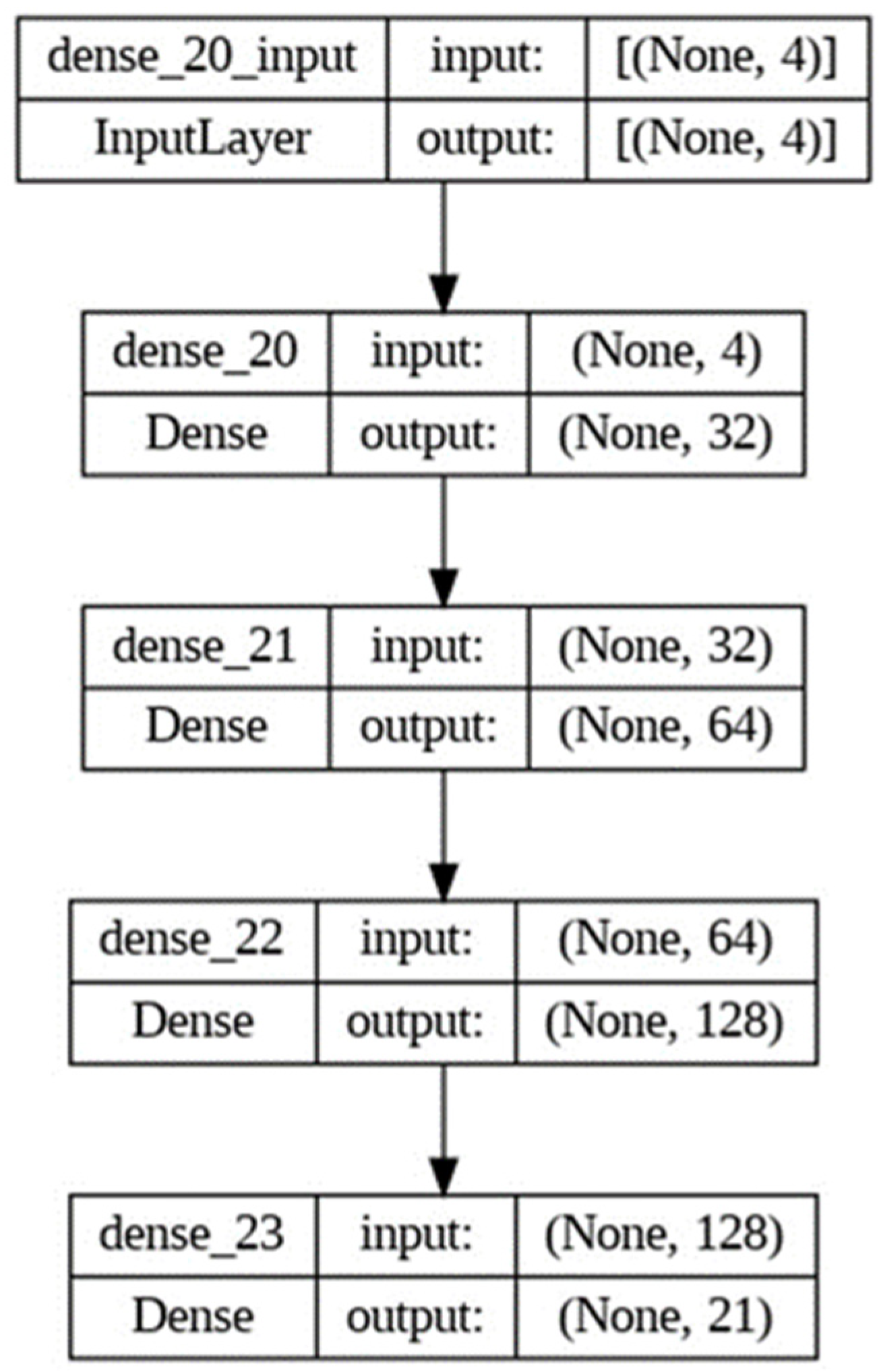
Using 1000 randomly generated noise arrays, 23,100 combinations of strain values for four measurement points containing noise were obtained and used to train the neural network. The network was trained only on the strain values observed at four strain measurement points and the load mass values, which were categorized into 21 categories: category 0 corresponds to a mass of 2500 kg and category 20 to a mass of 12,500 kg. Thus, the input data of the neural network were vertical strains (obtained from simulation or the sensors in the case of real operation) and the output data were specified load masses. There were no coordinate values in the training data. The temperature of the rail was taken into account indirectly, since the data were initially filtered by the value of 22 °C. The described data were divided into training and test samples at a standard 80/20 ratio. The scheme of the used neural network is shown in
Figure 3.
This neural network is a simple multilayer perceptron model consisting of four layers. The first fully connected input layer consists of neurons with the ReLU activation function and receives the strain value at four strain measurement points. The next three layers are also fully connected with the ReLU activation function, while the number of neurons gradually increases from 32 to 128. The last fully connected layer is the output layer and consists of 21 neurons with the softmax activation function, according to the number of classes. The neural network was trained for 40 epochs.


