A Sequence-Based Hybrid Ensemble Approach for Estimating Trail Pavement Roughness Using Smartphone and Bicycle Data

Abstract

Trail pavement roughness significantly impacts user experience and safety. Measuring roughness over large areas using traditional equipment is challenging and expensive. The utilization of smartphones and bicycles offers a more feasible approach to measuring trail roughness, but the current methods to capture data using these have accuracy limitations. While machine learning has the potential to improve accuracy, there have been few applications of real-time roughness evaluation. This study proposes a hybrid ensemble machine learning model that combines sequence-based modeling with support vector regression (SVR) to estimate trail roughness using smartphone sensor data mounted on bicycles. The hybrid model outperformed traditional methods like double integration and whole-body vibration in roughness estimation. For the 0.031 mi (50 m) segments, it reduced RMSE by 54–74% for asphalt concrete (AC) trails and 50–59% for Portland cement concrete (PCC) trails. For the 0.31 mi (499 m) segments, RMSE reductions of 37–60% and 49–56% for AC and PCC trails were achieved, respectively. Additionally, the hybrid model outperformed the base random forest model by 17%, highlighting the effectiveness of combining ensemble learning with sequence modeling and SVR. These results demonstrate that the hybrid model provides a cost-effective, scalable, and highly accurate alternative for large-scale trail roughness monitoring and assessment.

1. Introduction

1.1. Background

As more people are using designated trails, there is a growing need to plan and construct appropriate infrastructure facilities [1]. According to the Iowa Department of Transportation (DOT), trails are shared-use paths used by bikes, pedestrians, skaters, wheelchair users, and joggers that are physically isolated from motor vehicle traffic by an open space or barrier [2]. These trails could be paved or unpaved. There are commonly two types of paved trails: asphalt concrete (AC) and Portland cement concrete (PCC). Many agencies throughout the United States utilize manuals such as the American Association of State Highway and Transportation Officials (AASHTO) Guide for the Development of Bicycle Facilities as a guideline for the design of bike lanes, shared paths, and shared-use trails [3,4]. However, few tools exist to analyze the roughness of roads and streets as a criterion to determine bicycle facility investment priorities and to generate a bicycle suitability network map. Thus, there is a pressing need to develop a cycling quality-of-service model [5]. The development of a statistically correct, mainstream evaluation instrument such as a bicycle lane quality or level-of-service model could provide critical help to agencies in setting their priorities for bicycle facility development projects [5].

Pavement roughness is a critical factor in the design and maintenance of trails for motorized and non-motorized transportation, including bicycles [3]. Pavement roughness is an important factor to consider in the design and maintenance of trails, as it can significantly impact the safety and comfort of bicycle travel [6]. Properly addressing pavement roughness through the use of effective maintenance strategies can improve the overall cycling experience and encourage more use of the trail system.

The International Roughness Index (IRI) is one of the most commonly used measurements to assess the quality, performance, and roughness of pavements [7,8]. The IRI is based on the quarter-car system (QCS), which is calculated by employing a simulated vehicle traveling at 49.71 mph (80 km/h) [9]. This system computes the vertical displacements of a simulated spring, after which roughness data can be acquired by employing a variety of mathematical filters and algorithms [10]. While the IRI was originally developed for assessing the roughness of roadways traveled by motor vehicles, it remains one of the most widely used and standardized metrics for evaluating pavement roughness. As such, the IRI has been adapted and utilized in prior studies evaluating trail pavement roughness [1,11,12,13,14,15,16]. It can provide a useful interim roughness measure that establishes a baseline roughness measurement and can be compared across studies, until ideal bike trail-specific metrics are developed and standardized.

1.2. Related Works

Due to the need for cost-effective pavement roughness evaluation methods, recent studies have explored using smartphones as low-cost sensors. For example, several studies have mounted smartphones on motorized vehicles to estimate the IRI, reporting reasonable accuracy compared to reference methods [17,18,19,20,21]. While these vehicle-mounted smartphone methods show promise, they are confined to motorable roads. An emerging approach is using smartphones mounted on bicycles, which allows the roughness measurement on non-motorized infrastructure such as trails.

Some studies have estimated road pavement roughness using bicycle-mounted phones, such as [22]. However, Shtayat et al. evaluated roughness for only one street section based on smartphone accelerometer data, without comparing them to any reference IRI measurements. Another work found that using very short test sections of 10 m with a bike-mounted phone led to weak correlation with the reference IRI [23]. The short sections appeared to be sensitive to localized variations like small bumps that negatively impacted the accuracy of the roughness measurements.

Other works have focused specifically on determining trail roughness using bicycles and smartphones [14,24]. Titov and Schlegel [14,24] developed a machine learning model to classify trail roughness into three broad categories (smooth, suitable, unsuitable) based on accelerometer data, achieving 90% precision. However, no quantitative IRI values were computed. The coarse three-level classification may be insufficiently detailed for agencies to make meaningful maintenance decisions. Wage et al. [14] proposed a methodology for estimating the IRI and Dynamic Comfort Index (DCI) values using bicycle-mounted phone acceleration, but they did not validate their data against actual IRI measurements. Without rigorous validation, the accuracy is unclear.

While Zang et al. [16] did report a strong correlation (r = 0.893) between their bike-phone IRI method and a professional profiler, their approach was only tested at a constant bike speed of 15.5 km/h. It is unrealistic for riders to maintain an exact constant speed in practice, limiting real-world applicability.

In addition to smartphone-based approaches, recent advancements in image-based techniques have provided new possibilities for pavement roughness estimation. Aleadelat et al. proposed the use of a low-cost depth camera (Intel RealSense D435i) to measure the IRI across road segments, demonstrating an 83% correlation with measurements from a standard road profiler. This approach offers a cost-effective solution, particularly for local agencies with limited budgets [25]. Mahmoudzadeh et al. took a different approach by using an RGB-D sensor to capture both color and depth data for 3D surface reconstruction. Their system achieved a high correlation between the estimated IRI and manual rod-and-level measurements, showcasing the potential of RGB-D sensors as a low-cost, effective tool for pavement roughness estimation [26]. These methods do not rely on smartphones but use dedicated sensors to capture detailed surface data. However, they face challenges, particularly in outdoor environments, where lighting conditions and sensor limitations can affect data quality.

In summary, while bicycle-mounted smartphone methods show promise for trail roughness evaluation, published studies have shortcomings, including a lack of IRI validation, limited speed or roughness ranges tested, low accuracy, and unoptimized data processing techniques. Image-based methods, although effective in capturing detailed surface data, also face computational and environmental challenges. To address these limitations, this study investigates the use of machine learning models, which have had limited application in real-time pavement roughness evaluation, despite their potential to capture complex roughness relationships. A data-driven modeling approach may offer improvements over the empirical or statistical models used previously. The goal of this study is to develop a robust methodology for estimating the IRI measurements on trails under real-world variable conditions using smartphone and bicycle data, taking advantage of the capabilities of machine learning to enhance accuracy and provide a more comprehensive analysis of trail roughness.

1.3. Ensemble Machine Learning Models

Ensemble machine learning algorithms have been of increasing interest to the computational intelligence and machine learning communities during the past couple of decades [27]. This interest is well earned, since ensemble systems have demonstrated their superior performance and remarkable adaptability across a wide range of problem domains and practical applications [27]. Ensemble systems have successfully been used to address a variety of machine learning issues, including feature selection, confidence estimation, missing features, incremental learning, error correction, class imbalanced data, and learning concept drift from nonstationary distributions, among others [27]. Ensemble systems were initially developed to reduce the variance—thus improving the accuracy—of an automated decision-making system [27]. Ensemble algorithms are a generalized meta method to machine learning that aim to improve prediction accuracy by mixing predictions from many models [27,28]. There are three types of these algorithms: (1) bagging, (2) stacking, and (3) boosting. Bagging is a method of combining a number of tree cart models and combining the predictions of these models by averaging [28]. Random forests are an example of the bagging method. Stacking is the process of learning different models on a data set and then combining these models with another model that tries to learn how to combine these models [28]. Boosting is weighting the predictions and subsequently adding ensemble members that correct the predictions produced by earlier models [28]. Adaptive boosting and gradient boosting are examples of this method.

Random forest is an ensemble method that constructs multiple decision trees during training and outputs the mode of their predictions (for classification) or the mean prediction (for regression). The algorithm operates by creating a diverse set of trees through bootstrapping (sampling with replacement) and random feature selection at each split, which helps to reduce overfitting and improve generalization [29,30,31]. The fundamental equation governing the predictions of a random forest can be expressed as follows:

$$\mathrm{ŷ}={\displaystyle \frac{1}{N}}\sum _{i=1}^N{T}_i\left(x\right)$$

(1)

where $\mathrm{ŷ}$ is the predicted output, $T_i\left(x\right)$ represents the individual trees, and $N$ is the total number of trees in the forest. This method has been shown to be particularly effective in high-dimensional spaces and is robust against noise and overfitting [29,32].

Adaptive boosting is a boosting technique that aims to convert weak learners into strong learners. It does this by sequentially applying weak classifiers (often decision trees) and adjusting their weights based on the errors of previous classifiers. The algorithm focuses more on misclassified instances in subsequent iterations, thereby improving the model’s accuracy [33,34]. The core idea can be summarized by the following equation:

$$\mathrm{ŷ}\left(\mathrm{x}\right)=\sum _{\mathrm{m}=1}^{\mathrm{M}}{\mathsf{\alpha }}_{\mathrm{m}}{\mathrm{h}}_{\mathrm{m}}\left(\mathrm{x}\right)$$

(2)

where $\mathrm{ŷ}\left(\mathrm{x}\right)$ is the final output, ${\mathrm{h}}_{\mathrm{m}}\left(\mathrm{x}\right)$ denotes the weak classifiers, $\mathrm{M}$ is the number of weak classifiers, and ${\mathsf{\alpha }}_{\mathrm{m}}$ represents the weight assigned to each classifier based on its performance.

Gradient boosting is another powerful boosting method that builds models in a stage-wise fashion. Unlike adaptive boosting, which adjusts weights based on misclassification, gradient boosting optimizes a loss function by fitting new models to the residuals of the predictions made by the existing ensemble. The iterative process can be mathematically represented as follows:

$${\mathrm{ŷ}}_{\mathrm{m}}\left(\mathrm{x}\right)={\mathrm{ŷ}}_{\mathrm{m}-1}\left(\mathrm{x}\right)+\mathsf{\nu }\cdot {\mathrm{h}}_{\mathrm{m}}\left(\mathrm{x}\right)$$

(3)

where ${\mathrm{ŷ}}_{\mathrm{m}}\left(\mathrm{x}\right)$ is the prediction at the m-th iteration, ${\mathrm{ŷ}}_{\mathrm{m}-1}\left(\mathrm{x}\right)$ is the prediction from the previous iteration, $\mathsf{\nu }$ is the learning rate, and ${\mathrm{h}}_{\mathrm{m}}\left(\mathrm{x}\right)$ is the new model fitted to the residuals [30,35]. This method is particularly effective for complex data sets and has been widely adopted in various applications.

Ensemble algorithms have demonstrated superior performance for predicting pavement conditions across various studies [36,37,38,39]. However, these existing applications focused on forecasting future pavement deterioration using historical data for factors like age, traffic loading, and materials. The ensembles were not applied to estimate the current pavement condition from direct measurements. This distinction highlights a key novelty of the proposed approach of utilizing ensemble learning to measure real-time roughness from smartphone sensors. While ensembles have proven effective for pavement deterioration modeling, adopting them to enable roughness measurements represents a new application. The aim here is to leverage ensemble learning to improve the accuracy of present condition roughness estimates, which are critical for trail pavement management.

2. Materials and Methods

In this research, three distinct methods were utilized for the assessment of pavement roughness in relation to the IRI on trails. As depicted in Figure 1, the research encompasses the utilization of three methodological approaches: double integration, whole-body vibration, and machine learning. The incorporation of these three approaches serves the purpose of comparative analysis, seeking to identify the most appropriate technique for an accurate measurement of the IRI. The double integration method begins by applying a high-pass filter to the acceleration data recorded by the smartphone accelerometer. Double integration is then applied to convert acceleration to displacement. To improve data quality, the moving average filter and baseline correction filter are applied to the data. Subsequently, a mathematical model, referred to as the “bicycle model” in this paper, is used to estimate the IRI. Finally, a regression calibration model is adopted.

In the whole-body vibration method, after filtering the acceleration data with a high-pass filter, the method utilizes the root mean square of vertical acceleration and bicycle speed to model the relationship with the IRI as an empirical regression model.

The machine learning method utilizes the acceleration data along with other types of data and the bicycle model data from the double integration method to train a machine learning model. This method employs a sliding window technique and then utilizes a hybrid modeling technique to model the IRI.

The subsequent sections will expound upon the methodology applied for data collection, model development, and model evaluation.

2.1. Data Collection

The methodology for this research was applied to eight trail segments, each approximately 0.31 mi (499 m) in length, located in West Des Moines, Iowa. Four segments were asphalt concrete (AC): the Walnut Creek Trail (A1), Jordan Creek Trail (A2), Krudenier Trail (A3), and Carl Voss Trail (A4). The remaining four were Portland cement concrete (PCC): the John Pat Dorian Trail (C1), Jordan Creek Trail (C2), Meredith Trail (C3), and Easter Lake Trail (C4). The segments were selected based on their homogeneity in terms of condition and length. The IRI survey was conducted in 2022 using both a smartphone-mounted bicycle and a walking profiler, with each segment traversed four times (twice in each direction).

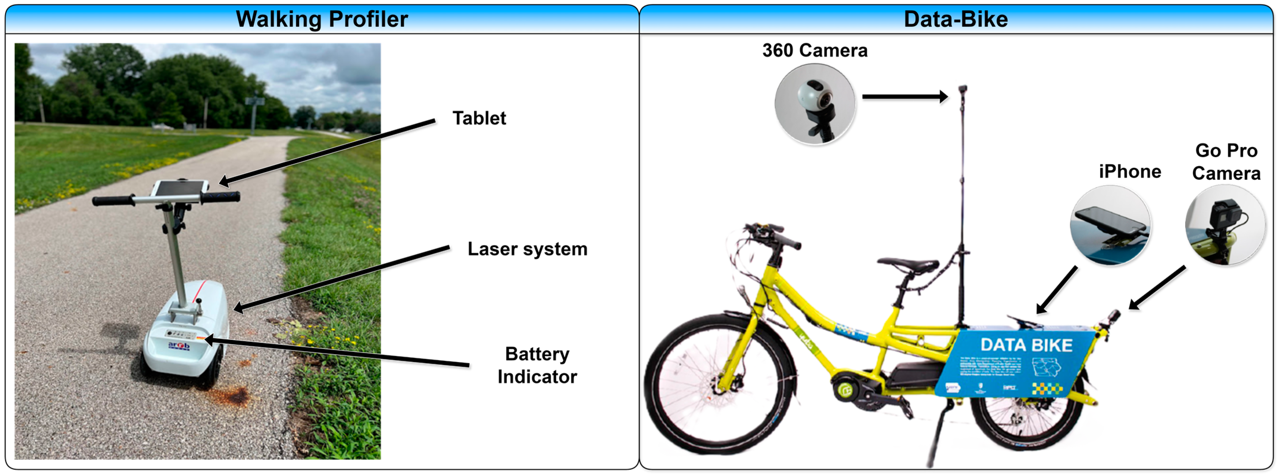
Two types of data collection methods were employed: a smartphone-mounted on a bicycle (as depicted in Figure 2) and a reference IRI device (Australian Road Research Board’s walking profiler). The walking profiler (as depicted in Figure 2) was used as the reference for both evaluating and calibrating the smartphone data. The data collection that was conducted on each segment included GPS data (latitude, longitude, speed), vibration data (x, y, z acceleration), magnetometer data (x, y, z axis), and orientation data (x, y, z axis).

2.2. Numerical Double Integration Method

In this approach, a second-degree Butterworth high-pass filter was applied to the collected vertical acceleration data from the smartphone accelerometer to filter out components with wavelengths above 30 m from the acceleration signals. The objective of this filter was to remove the undesired wavelength components, which are those not directly related to the calculation of the IRI. The cutoff frequency for this filter was determined using the formula specified in [40], as follows:

$$f={\displaystyle \frac{v}{\lambda }}$$

(4)

where $f$ is the cutoff frequency (Hz), $v$ is the average speed on the segment (m/s), and $\lambda$ = 30, which is the wavelength in meters ($\lambda$ = 67.108 mph/s when using $v$ in mph and the output $f$ in Hz).

After that, the filtered data were then numerically double-integrated into displacement data using the following equation:

$$D\left(t\right)=\underset{t=0}{\overset{t}{\iint }}{a}_z\left(t\right) {dt}^2$$

(5)

where $D\left(t\right)$ is the displacement in the time domain $t$, and $a_z\left(t\right)$ is the vertical acceleration in the time domain.

After obtaining the vertical displacement data using the previous equation, the baseline correction filter and finite impulse response (FIR) moving average filter were applied to the data. The baseline correction filter was adopted to remove the trend from the displacement data caused by the accumulated error during the double integration process. A Python package called “BaselineRemoval 0.1.1” was used to perform linear baseline correction [41]. The moving average filter was used to reduce the impact of accelerometer noise on the displacement data.

This approach assumes that the bicycle is a rigid structure with only one mass and no springs, in contrast to vehicle structures (QCS), which typically consist of two masses and springs. Consequently, the calculated vertical displacement of the bicycle is considered equivalent to the longitudinal profile, as described by [16]. Then, the roughness can be computed by dividing the sum of the difference in vertical displacements by the travel distance (segment length) according to the following equation:

$${BRI}_s=\frac{{\displaystyle {\sum }_{t=2}^t}\left|D\left(t\right)-D(t+1)\right|}{L}$$

(6)

where ${BRI}_s$ is the Bicycle Roughness Index based on the smartphone data, and $L$ is the segment length. The segment length could be measured from the GPS data using the following equation [16]:

$$L=\left(2\right)\left(R\right)\arcsin \left(\sqrt{{\sin }^2\left({\displaystyle \frac{{lat}_2-{lat}_1}{2}}\right)+\cos \left({lat}_1\right)\cos \left({lat}_2\right){\sin }^2\left({\displaystyle \frac{{long}_2-{long}_1}{2}}\right)}\right)$$

(7)

where ${lat}_2$ and ${lat}_1$ are latitude points, ${long}_2$ and ${long}_1$ are longitude points, and $R$ is the radius of the Earth, which is equal to about 6371 km.

After measuring the ${BRI}_s$, the following equation was used to calibrate the measured values from the double integration method with the walking profiler IRI:

$$IRI=b_1\left({BRI}_s\right)+b_2$$

(8)

where $IRI$ is the final calibrated IRI, and $b_1$ and $b_2$ are the calibration coefficients.

2.3. Whole-Body Vibration Method

International Organization for Standardization (ISO) 2631-1 is the reference standard for the definition of vibrations that are conveyed to the vehicle or bicycle body as a result of road conditions [42]. In line with this ISO standard, the vertical acceleration’s root mean square (RMS) for each segment was calculated in this study to indicate the pavement roughness as follows:

$$RMS=\sqrt{{\displaystyle \frac{\sum {\left(a_z\right)}^2}{n}}}$$

(9)

where $a_z$ (m/s²) is the vertical acceleration in the time domain after applying a high-pass filter using Equation (4), and $n$ is the number of vertical acceleration data points collected over the segment.

Many researchers have examined the impact of speed on the measured pavement roughness based on the QCS method such as [17,23,40,43,44,45]. The reference speed should be a factor in determining the IRI threshold levels. Taking into account the same whole-body vibration value of suspension relative to velocity, it is possible to attain the same degree of vibration response for two different velocities, v₁ and v₂ [46,47]. As a result, the relationship between the IRI threshold values and speed restriction could be given as follows [47]:

$${IRI}_{v2}=\left({IRI}_{v1}\right){\left({\displaystyle \frac{v_1}{v_2}}\right)}^{0.5}$$

(10)

By considering the RMS, Equation (10) will be transferred to the following according to Ahlin and Granlund [44]:

$${\displaystyle \frac{RMS}{IRI}}=0.16{\left({\displaystyle \frac{v}{80}}\right)}^{{\displaystyle \frac{w-1}{2}}}$$

(11)

However, these relationships were initially developed based on road profile inputs with a very specific assumed spectral character. It is improbable that the spectral content assumed in those experiments aligns with the conditions on the paths measured in this study. Consequently, an adjustment was made to the speed normalization equation originally proposed by those researchers, tailored to the specific trails investigated in our study. The subsequent equation serves a dual purpose in that it mitigates the influence of speed on pavement roughness and also calibrates the IRI obtained from the walking profiler method, given as follows:

$$IRI=b_1\left(RMS\right){\left({\displaystyle \frac{v_{th}}{v}}\right)}^{\alpha }+b_2$$

(12)

where $IRI$ is the walking profiler $IRI$, $v_{th}$ is the threshold speed (equal to 80 km/h or 49.71 mph), $v$ is the average speed on the segment, and $b_1$, $b_2$, and $\alpha$ are the calibration coefficients. The calibration coefficients were estimated using the reference IRI based on the Levenberg–Marquardt algorithm [48]. The threshold velocity ($v_{th}$) is set at 80 km/h (49.71 mph), which is the default speed for IRI estimation in the QCS method [49]. This value serves as a reference point for normalizing speeds across different road segments. When the actual speed ($v$) equals the threshold velocity, the speed adjustment factor becomes 1, indicating no adjustment is needed. For speeds below 80 km/h, the factor increases the adjusted IRI to compensate for a reduced dynamic response, while for speeds above 80 km/h, it decreases the adjusted IRI to account for an increased dynamic response. This approach enables a standardized comparison of pavement roughness across segments traveled at various speeds, with 80 km/h as the reference.

2.4. Hybrid Ensemble Machine Learning Method

In contrast to previous methods applied to the 0.31 mi (499 m) segments, this part of the study segmented the data into 0.031 mi (50 m) sections. The shorter length was chosen to obtain a greater number of data points for training the machine learning model, while still maintaining a reasonable section length for smartphone sensor accuracy. Specifically, GPS sensors on smartphones have been reported to have accuracy that can potentially exceed 10 m and up to 30 m in some cases [50,51]. To ensure reliable segmentation based on the GPS data, a conservative section length of 50 m was selected. The shorter segments are also hypothesized to help the machine learning model better capture local roughness variability. While conventional methods may smooth over such local changes, the machine learning approach is expected to characterize local roughness patterns within the segments.

Data from multiple smartphone sensor types were collected, including the accelerometer, gyroscope, magnetometer, and GPS sensors. As described previously, the accelerometer provided acceleration data, and the GPS gave location data used for calculating travel distance and for section segmentation. The gyroscope and the magnetometer were used to collect the smartphone’s local orientation and orientation in space, respectively. The local orientation measures the smartphone orientation according to its mounting position. However, the orientation in space measures the smartphone orientation with respect to the north. These two types of data were considered to capture exceptional events during data collection. For instance, abrupt shifts in the bicycle’s direction could influence the acceleration data, either due to pavement surface irregularities like cracks or potholes, or as a result of the cyclist’s actions, such as sudden turns or changes in direction.

The accelerometer provided data for the root mean square (RMS) values along the z-axis (${RMS}_z$), x-axis (${RMS}_x$), and y-axis (${RMS}_y$), as well as the maximum (${Max}_z$), minimum (${Min}_z$), and summation (${Sum}_z$) of acceleration on the z-axis. The GPS data were used to calculate the average speed ($V$), speed variance ($VarV$), and maximum speed ($MaxV$) over each segment. Gyroscope data included RMS values for orientation on the z-axis (${Gyro}_z$), x-axis (${Gyro}_x$), and y-axis (${Gyro}_y$), while the magnetometer provided RMS values for the z-axis (${Mag}_z$), x-axis (${Mag}_x$), and y-axis (${Mag}_y$). Additional input variables included the pavement type (either PCC or AC) and Bicycle Roughness Index (${BRI}_s$) values using the double integration method.

Figure 3 shows the flowchart of the methodology for developing the proposed hybrid model (where n is denoted as the section order). The hybrid modeling in this research comprised the following steps:

Firstly, train ensemble models (random forest) on the collected data and variables previously mentioned. These ensemble models are referred to as “Ensemble model (1)” in Figure 3 and are trained on the data set without considering sequential information. The data set was divided into two data sets: training and testing. The training set contained 80% of the overall data set, while the testing set contained 20%. The grid search method was used for hypertuning the hyperparameters of the selected models. The grid search algorithm is a thorough analysis of selecting the hyperparameters of machine learning models [52].

Secondly, apply the sliding window technique to the collected data and train a new ensemble model based on this technique. This technique considers the sequence order of the collected data and provides new input data to the model based on the previously collected data in the previous section. In Figure 3, this is represented by the “If n > 0” condition, where “Input n” contains data from the current trail section, and “Input n − 1” contains data from the previous section. It is believed that the pavement roughness of the current section is affected by the amount of pavement roughness in the previous section. This is due to the accumulated vertical movement in the bicycle when passing over pavement segments. The ensemble model trained using this sliding window technique is referred to as “Ensemble model (2)” in Figure 3.

Thirdly, feed the output values of “Ensemble model (2)” into a support vector regression (SVR) model. SVR is a type of robust machine learning technique that enables users to customize the level-of-error tolerance by defining an acceptable error margin and modifying the tolerance for exceeding that acceptable error rate [53,54]. Instead of minimizing the squared error, like with ordinary least squares (OLS) regression, the SVR’s objective function is to minimize the coefficients vector [54]. Instead, the error term is dealt with in the constraints, where the absolute error is set to less than or equal to a predetermined margin, known as the maximum error (epsilon) [54]. Epsilon may be adjusted to give the model the necessary level of precision [54]. The reason for the hybridization of the ensemble model with the SVR model is to provide more robustness against the outliers. It was found that SVR is a good estimator for regression problems when the data contain noise [46]. In Figure 3, the SVR model is shown in the Hybrid Model section, combining outputs from “Ensemble model (2)” to produce a final IRI prediction.

Fourthly, estimate the current IRI value based on the trained model in the first step of “Ensemble model (1)”. After training the hybrid model, the first section of each segment will not have IRI values due to the sliding window technique, which considers the values of BRI_s and RMS_z from the previous section. In order to resolve this problem, the trained model “Ensemble model (1)” in the first step is needed to estimate the IRI value. This is represented in Figure 3 by the Base Model section, which is used for the first section (n = 1) when no previous section data are available.

Lastly, test the trained models on the test data set to select the model that performed best on the testing set (20% of the overall data). To ensure the robustness of our validation, the 20% testing set was deliberately structured to be representative of the entire data set. This testing set includes an equal proportion of pavement type sections, with approximately 58% being asphalt concrete (AC) and 42% being Portland cement concrete (PCC), reflecting the overall composition of the data set. Moreover, the selection of data points within the testing set covered almost the full spectrum of IRI values observed in the study to validate the model’s accuracy and reliability across various pavement conditions.

2.5. Evaluating and Comparing Terms

For the machine learning models, including the base models and hybrid model, the following error term was used as a loss function to be optimized and for tuning the hyperparameters of the models:

$$MSE={\displaystyle \frac{1}{n}}\sum _i^{i=n}{\left({IRI}_p-{IRI}_a\right)}^2$$

(13)

where $MSE$ is the mean square error, ${IRI}_p$ is the predicted $IRI$ value from the model, ${IRI}_a$ is the actual $IRI$ value, and $n$ is the number of data points in the data set.

For evaluating and comparing the models, the root mean square error (RMSE) and goodness of fit (R²) were used for the terms, given, respectively, in the following equations:

$$RMSE=\sqrt[2]{{\displaystyle \frac{1}{n}}\sum _i^{i=n}{\left({IRI}_p-{IRI}_a\right)}^2}$$

(14)

$$R^2=1-{\displaystyle \frac{{\displaystyle {\sum }_i^{i=n}}{\left({IRI}_p-{IRI}_a\right)}^2}{{\displaystyle {\sum }_i^{i=n}}{\left(\overline{{IRI}_a}-{IRI}_a\right)}^2}}$$

(15)

where $\overline{{IRI}_a}$ is the mean of the actual IRI values in the data set. The benefit of using RMSE over MSE is that the unit of RMSE is the same as the IRI unit, which makes more sense when comparing different models. The R² was also used to support the selection decision because, in some cases, the RMSE might be sensitive to outliers [55].

The relative mean absolute error (MAE) was also employed to compare the proposed methods, offering a general perspective on the relative errors produced by each model. The MAE (%) is presented in the following equation:

$$MAE\left(\%\right)={\displaystyle \frac{100}{n}}\sum _i^{i=n}{\displaystyle \frac{Abs\left({IRI}_p-{IRI}_a\right)}{{IRI}_a}}$$

(16)

where $Abs$ is the absolute positive value of a given number.

2.6. Sensitivity Analysis

The goal of the sensitivity analysis was to determine how model output uncertainty may be allocated to the uncertainty in each input variable [56,57]. The impact of each input variable on the model performance can be investigated using a number of sensitivity analysis methods such as local sensitivity analysis (LSA), global sensitivity analysis (GSA), and extended Fourier amplitude sensitivity analysis (EFAST) [57]. Due to the complexity of the modeling approach adopted in this paper, not all of these methods are suitable to be implemented. For example, the LSA method cannot explain the impact of variables on the output when the relationship is non-linear [57]. Thus, a simple sensitivity analysis based on the error term was conducted in this paper. The method was adopted by a number of studies such as [58,59,60].

The following parameter ($W_i$) was measured after finalizing the training of the machine learning model [58,59,60]:

$$W_i={\displaystyle \frac{{MSE}_i}{{MSE}_f}}$$

(17)

where $W_i$ is the relative error term to investigate the importance of each variable, ${MSE}_i$ is the $MSE$ value from the model after excluding the variable, and ${MSE}_f$ is the $MSE$ value when all variables are included in the model.

This method considers the impact of each variable on the error term when excluding that variable from the model. When the ${MSE}_i$ value is high, the model is sensitive to that particular variable, and the variable is important for predicting the output. In order to make the results of this method more comparable, the authors of this paper added the following term to estimate the relative importance:

$${IMP\left(\%\right)}_i={\displaystyle \frac{W_i-1}{{\displaystyle {\sum }_i^{i=n}}\left(W_i-1\right)}}\times 100$$

(18)

where ${IMP\left(\%\right)}_i$ is the relative importance in percent for each selected variable in the data set. If $W_i$ < 1, then ${IMP\left(\%\right)}_i$ will be a negative value. A negative value means the input variable negatively affects the performance of the model. The opposite is also true such that if $W_i$ > 1, then ${IMP\left(\%\right)}_i$ will be a positive value. A positive value means the input variable positively affects the performance of the model.

The use of MSE, despite its sensitivity to small variations, is particularly valuable for its robustness in highlighting significant influences on the model’s output. This approach ensures that even subtle but potentially important variations are considered, providing a comprehensive evaluation of variable impacts. Additionally, the calculation of the relative importance (IMP (%)) of each variable helps mitigate the risk of overemphasizing minor changes, thereby maintaining a balanced perspective on their practical significance.

3. Results for Double Integration and Vibration-Based Methods

Table 1. The results of the developed regression models using the double integration and vibration- based methods.

Method	Trail Material	Model Equation		Evaluation
Double Integration	AC	$IRI=0.926\left({BRI}_s\right)-209.20$	(19)	R2 = 0.77, RMSE = 62.99
	PCC	$IRI=0.920\left({BRI}_s\right)-246.982$	(20)	R2 = 0.70, RMSE = 64.59
Vibration-Based	AC	$IRI=4.906\left(RMS\right){\left({\displaystyle \frac{49.71}{v}}\right)}^{1.882}+94.267$	(21)	R2 = 0.90, RMSE = 40.68
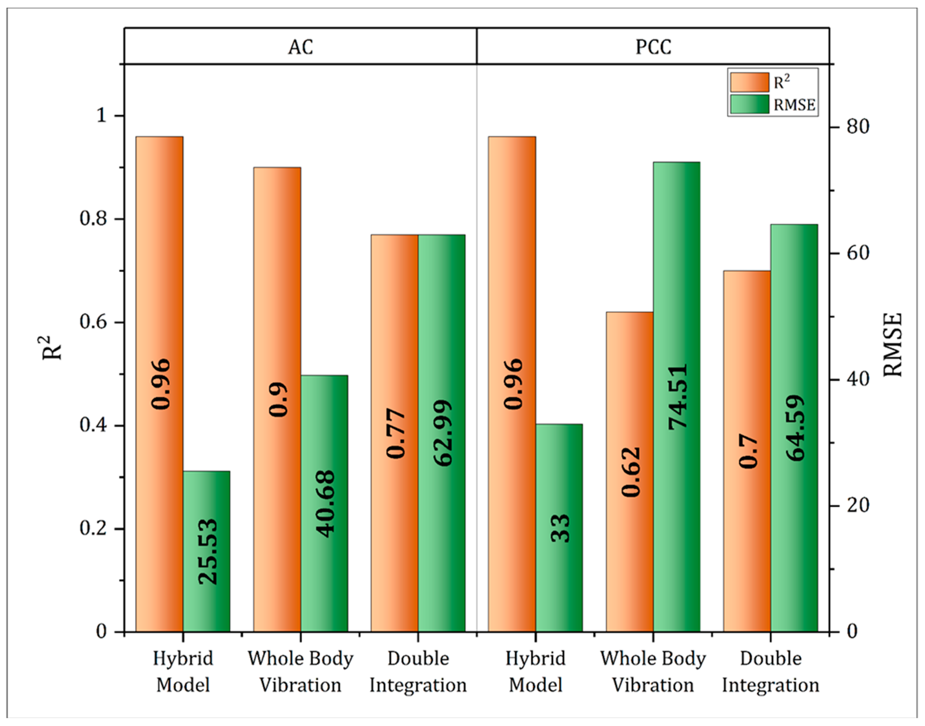
	PCC	$IRI=20.785\left(RMS\right){\left({\displaystyle \frac{49.71}{v}}\right)}^{1.179}+90.534$	(22)	R2 = 0.62, RMSE = 74.51

shows the results of the regression models that were developed for the AC and PCC trails (0.31 mi, 499 m segments) using the double integration and whole-body vibration methods. Where $IRI$ and ${BRI}_s$ are given in inch per mile (in/mi), and $RMS$ is given in meter per second square (m/s²). The R² and RMSE for Equation (19) are 0.77 and 62.99, and they are 0.90 and 40.68 for Equation (21), respectively. In this case, it could be concluded that the whole-body vibration method is better than the double integration method for AC trails. On the other hand, the R² and RMSE for Equation (20) are 0.70 and 64.59, and they are 0.62 and 74.51 for Equation (22), respectively. In contrast to the previous result, in this case the double integration method is better than the whole-body vibration method for PCC trails. This could be due to the transverse joints in PCC trails, which could affect the whole-body method’s vertical vibrations.

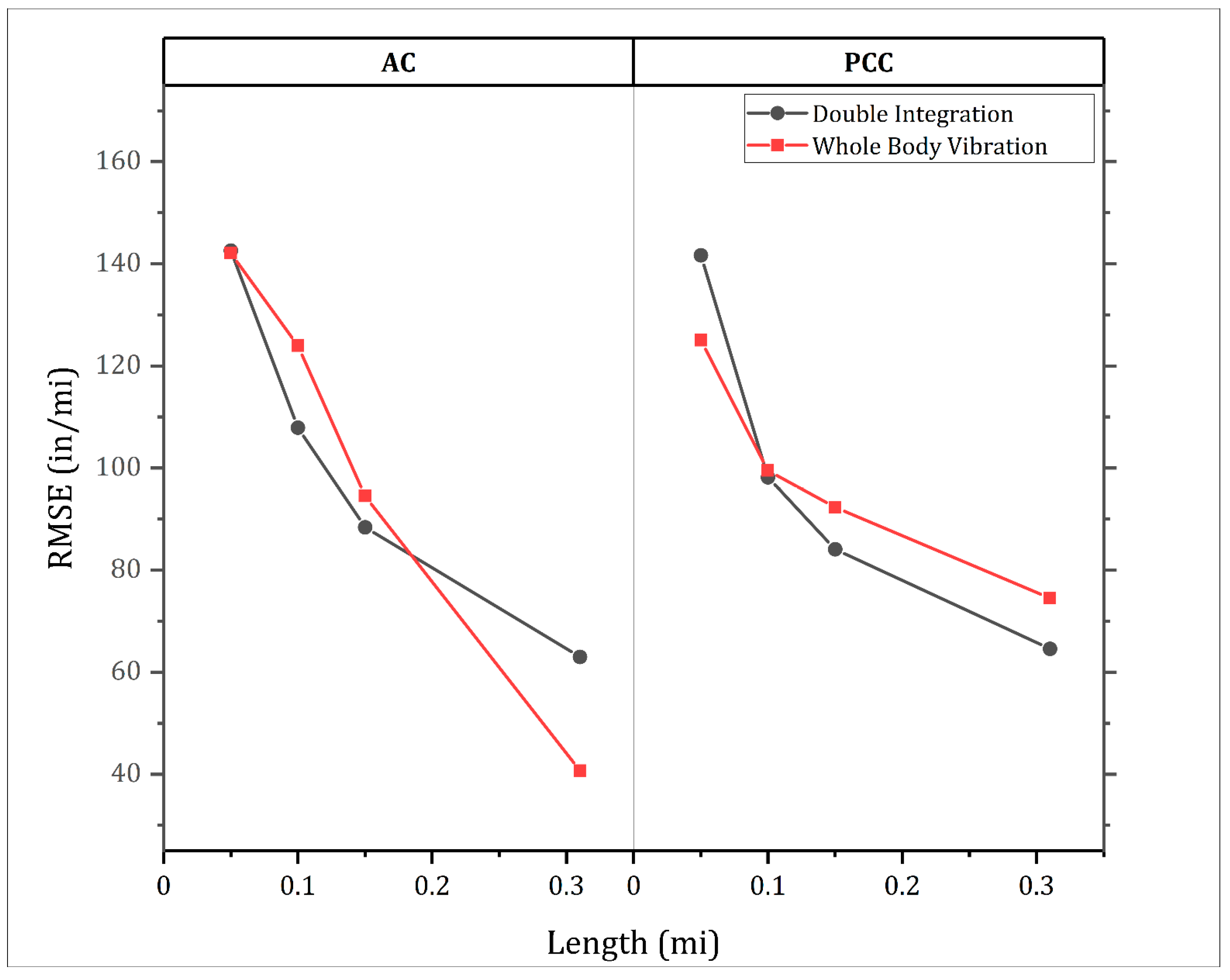
The same methodology was applied again to different section lengths (0.15, 0.1, and 0.05 mi) in order to investigate the impact of section length on the accuracy of the proposed methods. Figure 4 summarizes the results of the whole-body vibration and double integration methods for AC and PCC trails for segment lengths of 0.05–0.3 mi. It is clearly shown that when the section length decreases, the accuracy also decreases (RMSE increases). This observation aligns with the findings from other studies in the field. For instance, a study on smartphone-based IRI estimation found that the correlation between the IRI and root mean square of vertical acceleration (RMSVA) increased with segment length [61]. They reported Pearson’s correlation coefficient (r) values of 0.67, 0.78, 0.77, and 0.82 for segment lengths of 20, 100, 200, and 500 m, respectively.

Several factors may contribute to this phenomenon. Firstly, there is the uncertainty of the IRI measurements: As noted in [62], variations can occur in IRI measurements from run to run, especially when the contact area between the bicycle tire and the pavement is relatively small compared to road vehicles. Additionally, GPS sensor error plays a role; the accuracy of GPS sensors, particularly in smartphones, can affect the precision of location data for shorter segments. The referenced study also highlighted this as a potential factor in lower correlations for short segments [61]. Moreover, data aggregation effects come into play; longer segments allow for more data points to be aggregated, potentially smoothing out local variations and sensor noise, leading to more stable and accurate estimates. Furthermore, the crossing of data between devices is a consideration; the process of aligning data from different devices (e.g., smartphones and reference equipment) may introduce errors that are more pronounced in shorter segments [61]. When the section length is long enough, the impact of these factors could be reduced.

In this study, regression coefficients were estimated from eight trail segments, with four segments dedicated to each trail surface type as shown in Equations (19)–(21). However, to enhance the model’s applicability to different pavement types, further calibration across a broader range of pavement conditions would be beneficial. This approach would ensure that the model remains robust when applied to diverse environments, extending its utility without implying any inaccuracies in the original estimates.

4. Results for the Hybrid Ensemble Model

4.1. Base Models

The base three ensemble models including random forest, adaptive boosting, and gradient boosting were trained on the training data set with the help of the five-fold cross-validation and grid search methods for optimizing the hyperparameters of these models. The results of the training and testing are shown in

Table 2. The hyperparameter and the training and testing results of different ensemble learning models.

Model	Hyperparameters	Training Results	Testing Results
Random forest	Trees = 500 Depth of trees = 4 Subset split limit = 4	R2 = 0.80, RMSE = 85.53	R2 = 0.73, RMSE = 91.06
Adaptive boosting	Number of estimators = 5 Learning rate = 0.1 Random generator = 1000 Loss = ‘Square’	R2 = 0.95, RMSE = 41.10	R2 = 0.66, RMSE = 102.59
Gradient boosting	Number of estimators = 5 Learning rate = 0.15 Depth of trees = 3 Random generator = 1000	R2 = 0.79, RMSE = 88.90	R2 = 0.71, RMSE = 93.74

. According to these results, the highest model in terms of accuracy for training and testing was random forest. Gradient boosting showed an accuracy slightly lower than random forest. On the other hand, adaptive boosting was the lowest accuracy in the testing set. Despite the training accuracy being higher than other models, the testing accuracy was much lower than the training. Adaptive boosting, in this study, tended to overfit the training data, which is not a trivial problem and affects the reliability of the model. Given that it performed best, the random forest model was selected to conduct the next steps.

4.2. Hybrid Sequence-Based Model

After selecting the best performing model, the next steps were to perform the sliding window technique on the developed model and retrain the model based on the values of RMS_z and BRI_s in the previous section and then feed the SVR model with the outputs of the sequence-based model. After that, we could train and test the SVR model. The training and testing results for the hybrid model and hyperparameters are shown in

Table 3. The hyperparameters and the training and testing results for the hybrid model.

Model	Submodel	Hyperparameters	Training Results	Testing Results
Hybrid model	Sequence-based	Trees = 400 Depth of trees = 4 Subset split limit = 4	R2 = 0.85, RMSE = 76.16	R2 = 0.80, RMSE = 77.42
	SVR	C =1 ε = 0.5 Kernel = Polynomial

. Figure 5 shows the predicted IRI values from the hybrid model versus the actual values for the 0.031 mi (50 m) sections for the training and testing sets.

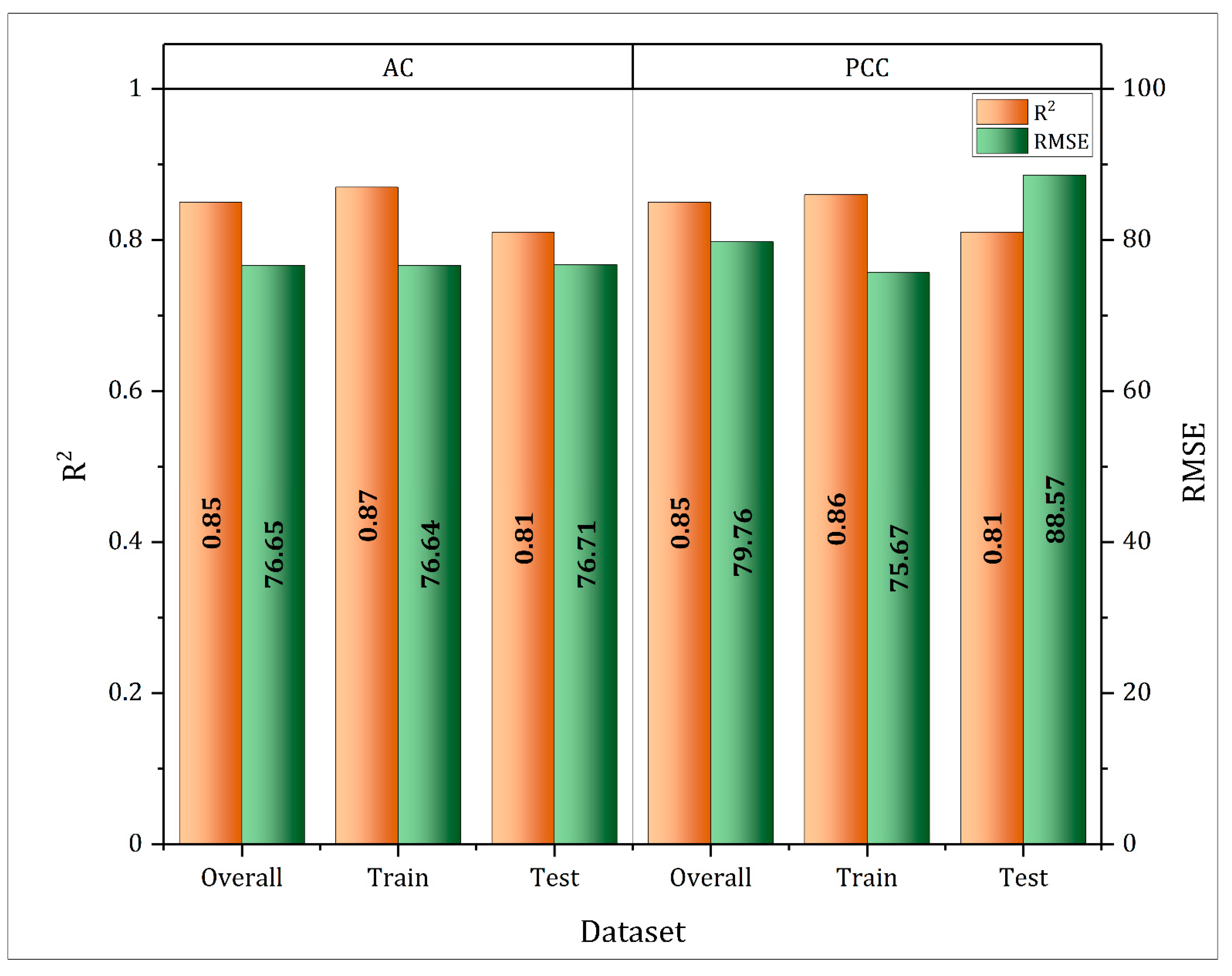
To further analyze the hybrid model’s performance, we conducted an individual investigation of its performance on both AC and PCC trails, as illustrated in Figure 6. Performance metrics, including R² and RMSE, were assessed for the overall, training, and testing sets, separately for the AC and PCC trails. The results revealed that the hybrid model performs slightly better on AC trails compared to PCC trails, which aligns with the findings of the double integration and whole-body vibration models. However, even on PCC trails, the hybrid model outperforms these models significantly.

It is important to note that these results pertain to the hybrid model without considering the first section of each segment. After combining the two proposed models—the first one for the initial section in each segment (ensemble model 1) and the second one for the remaining sections (ensemble model 2)—the R² and RMSE values were calculated as 0.85 and 75.53, respectively. Remarkably, these values closely resemble the results presented in Table 3.

4.3. Sensitivity Analysis Result

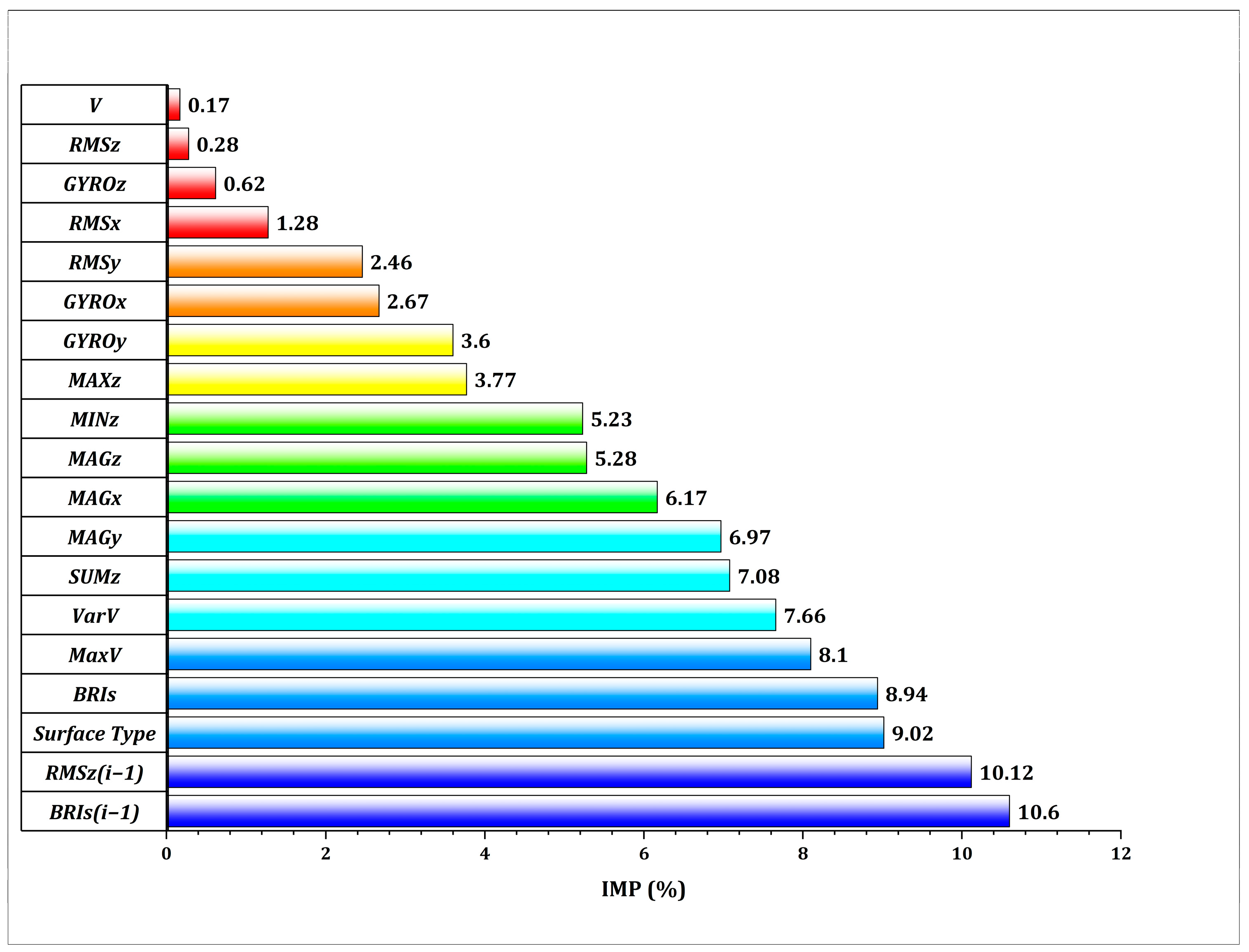
The sensitivity analysis, as outlined in the Materials and Methods Section, was performed on the final hybrid model to assess the impact of each variable on the model’s performance. Figure 7 displays the relative importance values of each input variable, along with the sequence-related variables for the preceding section (n − 1), RMS_z(n−1), and BRI_s(n−1). It is important to clarify that the purpose of this analysis is not to solely evaluate the IMP (%) value itself but to determine whether it has a positive or negative influence. In our results, all input variables exhibited positive IMP (%) values, suggesting that these variables have an impact on the model’s performance. However, it is worth noting that a positive IMP (%) value does not necessarily imply a positive effect; rather, it signifies that the variable affects the model’s output, and the direction of this effect can vary. Additionally, the sliding windows technique emerged as a noteworthy factor affecting the model’s performance based on the IMP (%) values of RMS_z(n−1), and BRI_s(n−1).

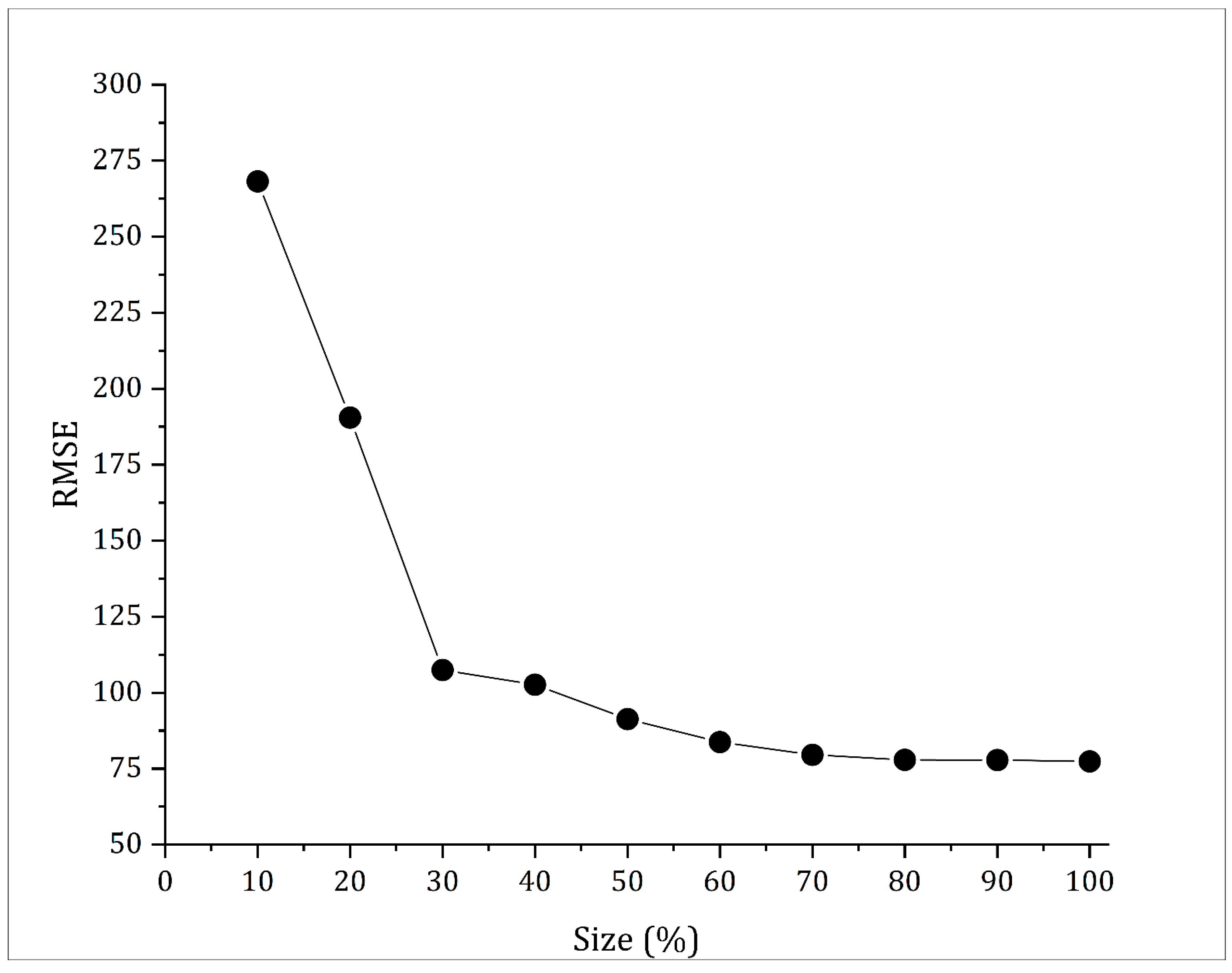
Another form of sensitivity analysis pertains to the data set size’s impact on the model’s performance. In this approach, the model underwent training with varying proportions of the training data set and was subsequently tested on the testing set. Figure 8 presents the relationship between the size of the training data set (in percentage) and the RMSE of the testing set. The graph illustrates that as the data set size increases, the model’s error (RMSE) decreases. This trend confirms the model’s capacity to capture and learn the intricate relationships between the input variables and the output variable. Notably, even when trained on as little as 70% of the data, the model retains its ability to predict the IRI with reasonable accuracy.

5. Comparison between the Proposed Methods

In this section, we compared the accuracy of the proposed methods: double integration, whole-body vibration, and the sequence-based hybrid ensemble model, specifically for PCC and AC trails, with segment lengths of 0.031 mi (50 m) and 0.31 mi (499 m). The comparison allows for the evaluation, practical application, and generalization of each method.

5.1. Segment Length: 0.31 mi (499 m)

First, the hybrid model was deployed on 0.031 mi (50 m) sections for each section in the evaluated segments. Then, the whole segment IRI was measured using the weighted average as follows:

$$IRI={\displaystyle \frac{{\displaystyle {\sum }_{i=1}^{i=n}}\left({IRI}_i\right)\left(L_i\right)}{{\displaystyle {\sum }_{i=1}^{i=n}}\left(L_i\right)}}$$

(23)

where $IRI$ (in./mi) is the $IRI$ for the 0.31 mi (499 m) segments, ${IRI}_i$ (in./mi) is the $IRI$ for the 0.031 mi (50 m) sections, and $L_i$ is the length of the section in the unit of miles.

Consequently, the R², RMSE, and MAE (%) were measured for the three models on each segment of the evaluated segments for AC and PCC trails. These results are shown in Figure 9 for R² and RMSE and in Figure 10 for MAE. From these figures, it can be concluded that the hybrid model is more accurate than other methods for both PCC and AC trails when evaluating 0.31 mi (499 m) segments. The RMSE of the hybrid model was about 60% and 37% lower than the double integration and whole-body vibration methods for AC trails, respectively. For PCC, it was about 49% and 56% lower than the double integration and whole-body vibration methods, respectively.

The MAE results are presented in Figure 10 for complementary analysis, although the RMSE was used as the primary model evaluation metric. Compared to the RMSE, the MAE has limitations for model selection but provides useful information on absolute error magnitudes [55]. The MAE analysis further revealed the hybrid model as the most accurate for both AC and PCC trails. The average percent accuracy was 93.6% and 92.8% for the hybrid model on AC and PCC trails, respectively.

Figure 11 plots the predicted IRI from each model versus the reference IRI for all sections in ascending order. The double integration and vibration methods exhibit substantial fluctuation in error, with average deviations from the reference IRI of up to 57 in./mi. In contrast, the hybrid model maintains errors within approximately 24 in./mi across sections. For instance, at trail section number 7 (PCC), the whole-body vibration model underestimates the IRI by approximately 90 in./mi, while the hybrid model stays within 11 in./mi of the true value. By reducing the fluctuations in error, the hybrid model provides more robust IRI estimates compared to the benchmark methods.

5.2. Segment Length: 0.031 mi (50 m)

The above comparison results only considered 0.31 mi (499 m) segments. The comparison for IRI values predicted using the proposed methods on 0.03 mi sections in terms of the RMSE and R² is shown in Figure 12. It is clearly shown by looking at the RMSE and R² values that the hybrid model outperformed the conventional methods by a huge margin. The RMSE for the hybrid model for AC trails is less than the double integration and whole-body vibration models by about 74% and 54%, respectively. The RMSE for the hybrid model for PCC trails is less than the double integration and whole-body vibration models by about 59% and 50%, respectively. The whole-body vibration model seems to be more robust than the double integration model, which appeared to be sensitive to smaller section lengths. The R² value for PCC trails, 0.031 mi sections, using the double integration model, reached almost zero (0.06). This is an indication that this method is not able to describe the variability in the data for PCC trails if the evaluation section is 0.031 mi.

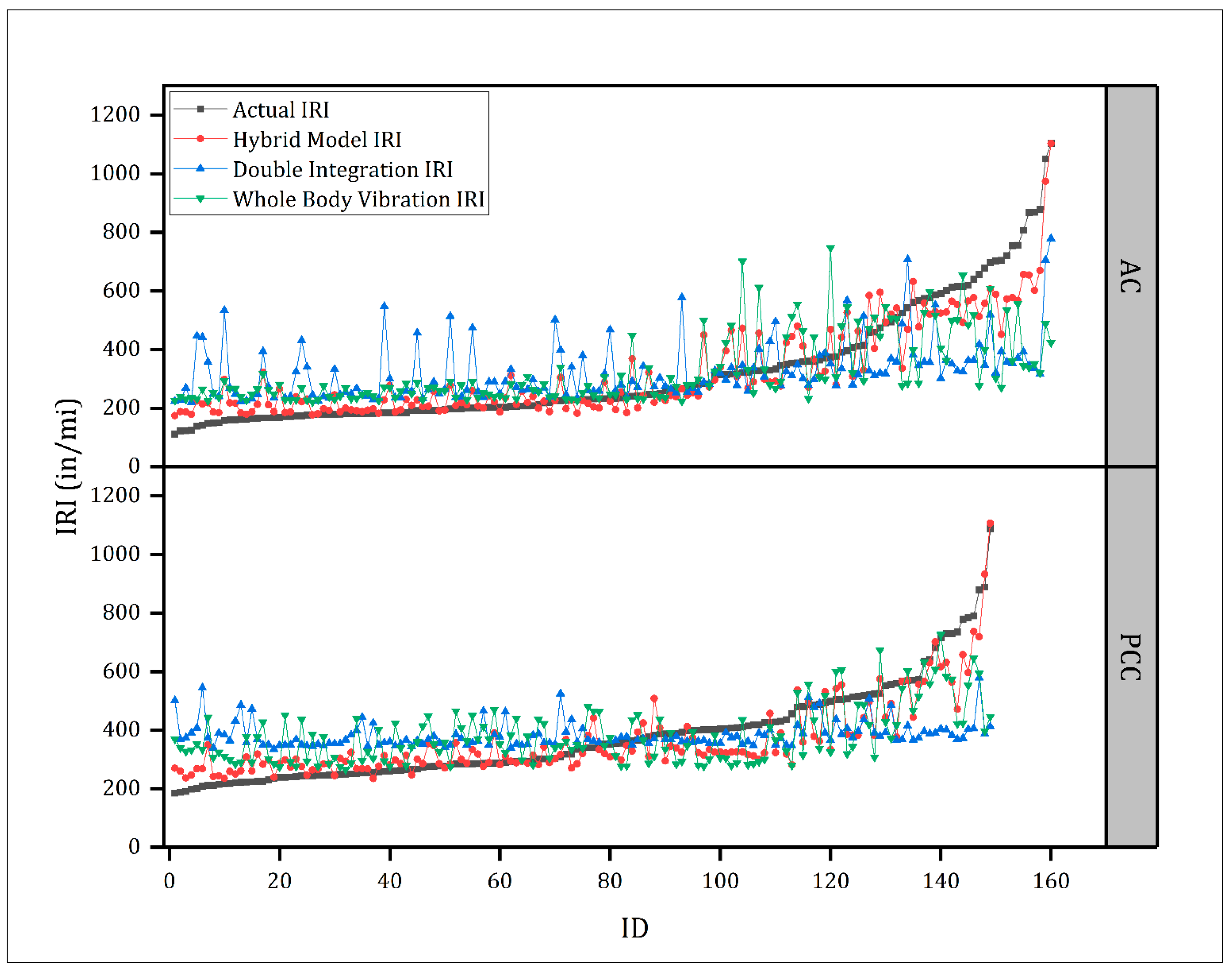
The IRI predicted values from each model and the actual IRI were plotted in ascending order versus the number (ID) of each section (0.031 mi, 50 m sections). As shown in Figure 13, it can be concluded that the accuracy of the double integration and whole-body vibration methods fluctuated. Moreover, they did not completely follow the pattern of the actual IRI. On the other hand, the hybrid model seems to be more robust for predicting the IRI compared to these two methods. This result is consistent with the previous results in Figure 11. However, all of these models were better using the longer 0.31 mi (499 m) segments.

6. Conclusions

This study introduces a novel hybrid ensemble machine learning model that significantly enhances trail pavement roughness estimations using smartphone-equipped bicycles. By integrating sequence-based modeling with support vector regression (SVR), the proposed model consistently outperformed traditional methods such as double integration and whole-body vibration across various trail types and segment lengths. For the 0.031 mi (50 m) segments, the hybrid model achieved a 54–74% reduction in the RMSE for asphalt concrete (AC) trails and a 50–59% reduction for Portland cement concrete (PCC) trails. Similarly, for the 0.31 mi (499 m) segments, RMSE reductions of 37–60% for AC trails and 49–56% for PCC trails were observed. These results demonstrate the model’s superior ability to capture local roughness variability, which is crucial for high-resolution pavement condition assessment.

When comparing the base ensemble models, the random forest algorithm performed best among the tested models, showing higher accuracy than adaptive boosting and gradient boosting. However, even the best-performing random forest model could not match the precision of the hybrid model. The hybrid model reduced the RMSE by 17% over the best base model, demonstrating that the combination of ensemble learning with sequence modeling and SVR can significantly enhance predictive accuracy.

In conclusion, this hybrid ensemble machine learning model represents a significant advancement in pavement condition assessment technology. Its ability to provide an accurate, scalable, and cost-effective roughness estimation offers a valuable tool for infrastructure management and maintenance planning. With further refinement, this approach has the potential to become a standard method for real-time trail condition monitoring across various non-motorized infrastructure systems, ultimately contributing to improved safety and user experience on trail networks.

References

1. Lin, W.; Dong, Y.; Ren, X.; Han, H.; Jung, Y. Development and Application of Riding Profiler for Roughness Evaluation on Bicycle Riding Surfaces. Sens. Mater. 2022, 34, 2709. [Google Scholar] [CrossRef]
2. IOWA DOT Iowa Department of Transportation (DOT)—IOWA BIKES INTERACTIVE MAP. Available online: https://iowadot.gov/iowabikes/bikemap/home.aspx (accessed on 25 December 2022).
3. AASHTO. Guide for the Development of Bicycle Facilities, 4th ed.; American Association of State Highway and Transportation Officials: Washington, DC, USA, 2012. [Google Scholar]
4. Landis, B.W.; Petritsch, T.A.; Huang, H.F.; Do, A.H. Characteristics of Emerging Road and Trail Users and Their Safety. Transp. Res. Rec. J. Transp. Res. Board 2004, 1878, 131–139. [Google Scholar] [CrossRef]
5. Landis, B.W.; Vattikuti, V.R.; Brannick, M.T. Real-Time Human Perceptions: Toward a Bicycle Level of Service. Transp. Res. Rec. J. Transp. Res. Board 1997, 1578, 119–126. [Google Scholar] [CrossRef]
6. Bíl, M.; Andrášik, R.; Kubeček, J. How Comfortable Are Your Cycling Tracks? A New Method for Objective Bicycle Vibration Measurement. Transp. Res. Part C Emerg. Technol. 2015, 56, 415–425. [Google Scholar] [CrossRef]
7. Hosseini, S.A.; Smadi, O. How Prediction Accuracy Can Affect the Decision-Making Process in Pavement Management System. Infrastructures 2021, 6, 28. [Google Scholar] [CrossRef]
8. Al-Suleiman (Obaidat), T.I.; Alatoom, Y.I. Development of Pavement Roughness Regression Models Based on Smartphone Measurements. J. Eng. Des. Technol. 2022, 22, 1136–1157. [Google Scholar] [CrossRef]
9. Sayers, M.W. The International Road Roughness Experiment: Establishing Correlation and a Calibration Standard for Measurements; University of Michigan, Ann Arbor, Transportation Research Institute: Ann Arbor, MI, USA, 1986. [Google Scholar]
10. Sayers, M.W. On the Calculation of International Roughness Index from Longitudinal Road Profile. Transp. Res. Rec. 1995. Available online: https://trid.trb.org/View/452992 (accessed on 4 October 2024).
11. Thigpen, C.G.; Li, H.; Handy, S.L.; Harvey, J. Modeling the Impact of Pavement Roughness on Bicycle Ride Quality. Transp. Res. Rec. J. Transp. Res. Board 2015, 2520, 67–77. [Google Scholar] [CrossRef]
12. Larsson, M.; Niska, A.; Erlingsson, S.; Tunholm, M.; Andrén, P. Condition Assessment of Cycle Path Texture and Evenness Using a Bicycle Measurement Trailer. Int. J. Pavement Eng. 2023, 24, 2262085. [Google Scholar] [CrossRef]
13. Rizelioğlu, M.; Yazıcı, M. New Approach to Determining the Roughness of Bicycle Roads. Transp. Res. Rec. J. Transp. Res. Board 2023, 2678, 781–793. [Google Scholar] [CrossRef]
14. Wage, O.; Feuerhake, U.; Koetsier, C.; Ponick, A.; Schild, N.; Beening, T.; Dare, S. Ride Vibrations: Towards Comfort-Based Bicycle Navigation. Int. Arch. Photogramm. Remote Sens. Spat. Inf. Sci. 2020, XLIII-B4-2020, 367–373. [Google Scholar] [CrossRef]
15. Niska, A.M.; Sjogren, L.; Weber, C.; De Jong, T.; Fyhri, A. Determination of Riding Comfort on Cycleways Using a Smartphone App. SSRN Electron. J. 2022. [Google Scholar] [CrossRef]
16. Zang, K.; Shen, J.; Huang, H.; Wan, M.; Shi, J. Assessing and Mapping of Road Surface Roughness Based on GPS and Accelerometer Sensors on Bicycle-Mounted Smartphones. Sensors 2018, 18, 914. [Google Scholar] [CrossRef] [PubMed]
17. Alatoom, Y.I.; Obaidat, T.I. Measurement of Street Pavement Roughness in Urban Areas Using Smartphone. Int. J. Pavement Res. Technol. 2022, 15, 1003–1020. [Google Scholar] [CrossRef]
18. Janani, L.; Doley, R.; Sunitha, V.; Mathew, S. Precision Enhancement of Smartphone Sensor-Based Pavement Roughness Estimation by Standardizing Host Vehicle Speed. Can. J. Civ. Eng. 2022, 49, 716–730. [Google Scholar] [CrossRef]
19. Sandamal, R.M.K.; Pasindu, H.R. Applicability of Smartphone-Based Roughness Data for Rural Road Pavement Condition Evaluation. Int. J. Pavement Eng. 2022, 23, 663–672. [Google Scholar] [CrossRef]
20. Yang, X.; Hu, L.; Ahmed, H.U.; Bridgelall, R.; Huang, Y. Calibration of Smartphone Sensors to Evaluate the Ride Quality of Paved and Unpaved Roads. Int. J. Pavement Eng. 2022, 23, 1529–1539. [Google Scholar] [CrossRef]
21. Zhang, Z.; Zhang, H.; Xu, S.; Lv, W. Pavement Roughness Evaluation Method Based on the Theoretical Relationship between Acceleration Measured by Smartphone and IRI. Int. J. Pavement Eng. 2022, 23, 3082–3098. [Google Scholar] [CrossRef]
22. Shtayat, A.; Moridpour, S.; Best, B.; Shahriar Rumi, M. Using a Smartphone Software and a Regular Bicycle to Monitor Pavement Health Statues. In Proceedings of the 2020 2nd International Conference on Robotics Systems and Vehicle Technology; Xiamen, China, 3–5 December 2020, Association for Computing Machinery: New York, NY, USA, 2020; pp. 121–126. [Google Scholar]
23. Cafiso, S.; di Graziano, A.; Marchetta, V.; Pappalardo, G. Urban Road Pavements Monitoring and Assessment Using Bike and E-Scooter as Probe Vehicles. Case Stud. Constr. Mater. 2022, 16, e00889. [Google Scholar] [CrossRef]
24. Titov, W.; Schlegel, T. Monitoring Road Surface Conditions for Bicycles—Using Mobile Device Sensor Data from Crowd Sourcing. Proceedings of the 5th International Conference, MobiTAS 2023, 25th HCI International Conference, HCII 2023, Copenhagen, Denmark, 23–28 July 2023, Krömker, H., Ed.; Springer International Publishing: Cham, Switzerland, 2019; 340–356. [Google Scholar]
25. Aleadelat, W.; Aledealat, K.; Ksaibati, K. Estimating Pavement Roughness Using a Low-Cost Depth Camera. Int. J. Pavement Eng. 2022, 23, 4923–4930. [Google Scholar] [CrossRef]
26. Mahmoudzadeh, A.; Golroo, A.; Jahanshahi, M.R.; Firoozi Yeganeh, S. Estimating Pavement Roughness by Fusing Color and Depth Data Obtained from an Inexpensive RGB-D Sensor. Sensors 2019, 19, 1655. [Google Scholar] [CrossRef]
27. Polikar, R. Ensemble Learning. In Ensemble Machine Learning: Methods and Applications; Zhang, C., Ma, Y., Eds.; Springer: Boston, MA, USA, 2012; pp. 1–34. ISBN 978-1-4419-9326-7. [Google Scholar]
28. Brownlee, J. A Gentle Introduction to Ensemble Learning Algorithms. Available online: https://machinelearningmastery.com/tour-of-ensemble-learning-algorithms/ (accessed on 13 December 2022).
29. Ustuner, M.; Balik Sanli, F. Polarimetric Target Decompositions and Light Gradient Boosting Machine for Crop Classification: A Comparative Evaluation. ISPRS Int. J. Geoinf. 2019, 8, 97. [Google Scholar] [CrossRef]
30. Kadiyala, A.; Kumar, A. Applications of Python to Evaluate the Performance of Bagging Methods. Environ. Prog. Sustain. Energy 2018, 37, 1555–1559. [Google Scholar] [CrossRef]
31. Alatoom, Y.I.; Al-Hamdan, A.B. A Comparative Study Between Different Machine Learning Algorithms for Estimating the Vehicular Delay at Signalized Intersections. J. Soft Comput. Civ. Eng. 2024, 123–160. Available online: https://www.jsoftcivil.com/article_196451.html (accessed on 4 October 2024).
32. Chan, J.C.-W.; Paelinckx, D. Evaluation of Random Forest and Adaboost Tree-Based Ensemble Classification and Spectral Band Selection for Ecotope Mapping Using Airborne Hyperspectral Imagery. Remote Sens. Environ. 2008, 112, 2999–3011. [Google Scholar] [CrossRef]
33. Yao, P.; Liu, Z.; Wang, Z.; Bu, S. Fault Signal Classification Using Adaptive Boosting Algorithm. Electron. Electr. Eng. 2012, 18, 97–100. [Google Scholar] [CrossRef]
34. Acula, D.D. Classification of Disaster Risks in the Philippines Using Adaptive Boosting Algorithm with Decision Trees and Support Vector Machine as Based Estimators. J. Model. Simul. Mater. 2021, 4, 7–18. [Google Scholar] [CrossRef]
35. Mayr, A.; Binder, H.; Gefeller, O.; Schmid, M. The Evolution of Boosting Algorithms. Methods Inf. Med. 2014, 53, 419–427. [Google Scholar] [CrossRef]
36. Sharma, A.; Sachdeva, S.N.; Aggarwal, P. Predicting IRI Using Machine Learning Techniques. Int. J. Pavement Res. Technol. 2023, 16, 128–137. [Google Scholar] [CrossRef]
37. Bral, S.; Kumar, P.P.; Chopra, T. Prediction of International Roughness Index Using CatBooster and Shap Values. Int. J. Pavement Res. Technol. 2022, 17, 518–533. [Google Scholar] [CrossRef]
38. Guo, R.; Fu, D.; Sollazzo, G. An Ensemble Learning Model for Asphalt Pavement Performance Prediction Based on Gradient Boosting Decision Tree. Int. J. Pavement Eng. 2022, 23, 3633–3646. [Google Scholar] [CrossRef]
39. Guo, W.; Zhang, J.; Cao, D.; Yao, H. Cost-Effective Assessment of in-Service Asphalt Pavement Condition Based on Random Forests and Regression Analysis. Constr. Build. Mater. 2022, 330, 127219. [Google Scholar] [CrossRef]
40. Chou, C.-P.; Siao, G.-J.; Chen, A.-C.; Lee, C.-C. Algorithm for Estimating International Roughness Index by Response-Based Measuring Device. J. Transp. Eng. Part B Pavements 2020, 146, 04020031. [Google Scholar] [CrossRef]
41. Haque, M.A. BaselineRemoval. GitHub Repository. 2022. Available online: https://github.com/StatguyUser/BaselineRemoval (accessed on 4 October 2024).
42. ISO 2631-1; Mechanical Vibration and Shock—Evaluation of Human Exposure to Whole-Body Vibration—Part 1: General Requirements, 2nd ed. International Organization for Standardization: Geneva, Switzerland, 1997.
43. Zeng, H.; Park, H.; Fontaine, M.D.; Smith, B.L.; McGhee, K.K. Identifying Deficient Pavement Sections by Means of an Improved Acceleration-Based Metric. Transp. Res. Rec. J. Transp. Res. Board 2015, 2523, 133–142. [Google Scholar] [CrossRef]
44. Ahlin, K.; Granlund, N.O.J. Relating Road Roughness and Vehicle Speeds to Human Whole Body Vibration and Exposure Limits. Int. J. Pavement Eng. 2002, 3, 207–216. [Google Scholar] [CrossRef]
45. Loprencipe, G.; Zoccali, P.; Cantisani, G. Effects of Vehicular Speed on the Assessment of Pavement Road Roughness. Appl. Sci. 2019, 9, 1783. [Google Scholar] [CrossRef]
46. Sun, L.; Zhang, Z.; Ruth, J. Modeling Indirect Statistics of Surface Roughness. J. Transp. Eng. 2001, 127, 105–111. [Google Scholar] [CrossRef]
47. Múčka, P. International Roughness Index Specifications around the World. Road Mater. Pavement Des. 2017, 18, 929–965. [Google Scholar] [CrossRef]
48. Levenberg, K. A method for the solution of certain non-linear problems in least squares. Q. Appl. Math. 1944, 2, 164–168. [Google Scholar] [CrossRef]
49. Uddin, W.; Hudson, W.; Elkins, G. Surface-Smoothness Evaluation and Specifications for Flexible Pavements. In Surface Characteristics of Roadways: International Research and Technologies; ASTM International: West Conshohocken, PA, USA, 1990; pp. 224–236. [Google Scholar]
50. Blum, J.R.; Greencorn, D.G.; Cooperstock, J.R. Smartphone Sensor Reliability for Augmented Reality Applications. In Proceedings of the Mobile and Ubiquitous Systems: Computing, Networking, and Services; Melbourne, VIC, Australia, 14–17 November 2023, Zheng, K., Li, M., Jiang, H., Eds.; Springer: Berlin/Heidelberg, Germany, 2013; pp. 127–138. [Google Scholar]
51. Merry, K.; Bettinger, P. Smartphone GPS Accuracy Study in an Urban Environment. PLoS ONE 2019, 14, e0219890. [Google Scholar] [CrossRef]
52. Liashchynskyi, P.; Liashchynskyi, P. Grid Search, Random Search, Genetic Algorithm: A Big Comparison for NAS. arXiv 2019, arXiv:1912.06059. [Google Scholar]
53. Smola, A.J.; Schölkopf, B. A Tutorial on Support Vector Regression. Stat. Comput. 2004, 14, 199–222. [Google Scholar] [CrossRef]
54. Sharp, T. An Introduction to Support Vector Regression (SVR). Available online: https://towardsdatascience.com/an-introduction-to-support-vector-regression-svr-a3ebc1672c2 (accessed on 13 December 2022).
55. Chai, T.; Draxler, R.R. Root Mean Square Error (RMSE) or Mean Absolute Error (MAE)?—Arguments against Avoiding RMSE in the Literature. Geosci. Model. Dev. 2014, 7, 1247–1250. [Google Scholar] [CrossRef]
56. Saltelli, A.; Sobol’, I.M. About the Use of Rank Transformation in Sensitivity Analysis of Model Output. Reliab. Eng. Syst. Safety 1995, 50, 225–239. [Google Scholar] [CrossRef]
57. Zhang, P. A Novel Feature Selection Method Based on Global Sensitivity Analysis with Application in Machine Learning-Based Prediction Model. Appl. Soft Comput. 2019, 85, 105859. [Google Scholar] [CrossRef]
58. Mrzygłód, B.; Hawryluk, M.; Janik, M.; Olejarczyk-Wożeńska, I. Sensitivity Analysis of the Artificial Neural Networks in a System for Durability Prediction of Forging Tools to Forgings Made of C45 Steel. Int. J. Adv. Manuf. Technol. 2020, 109, 1385–1395. [Google Scholar] [CrossRef]
59. Alatoom, Y.I.; Al-Suleiman (Obaidat), T.I. Development of Pavement Roughness Models Using Artificial Neural Network (ANN). Int. J. Pavement Eng. 2022, 23, 4622–4637. [Google Scholar] [CrossRef]
60. Ehsani, M.; Hamidian, P.; Hajikarimi, P.; Moghadas Nejad, F. Optimized Prediction Models for Faulting Failure of Jointed Plain Concrete Pavement Using the Metaheuristic Optimization Algorithms. Constr. Build. Mater. 2023, 364, 129948. [Google Scholar] [CrossRef]
61. Bisconsini, D.R.; Pegorini, V.; Casanova, D.; de Oliveira, R.A.; Farias, B.A.; Júnior, J.L.F. Intervening Factors in Pavement Roughness Assessment with Smartphones: Quantifying the Effects and Proposing Mitigation. J. Transp. Eng. Part B Pavements 2021, 147, 04021051. [Google Scholar] [CrossRef]
62. Jia, X.; Huang, B.; Zhu, D.; Dong, Q.; Woods, M. Influence of Measurement Variability of International Roughness Index on Uncertainty of Network-Level Pavement Evaluation. J. Transp. Eng. Part B Pavements 2018, 144, 04018007. [Google Scholar] [CrossRef]
Figure 1. The general methodology of the current research.
Infrastructures 09 00179 g001
Figure 2. The data-bike system used to collect smartphone sensor data and the walking profiler used to collect IRI values.
Infrastructures 09 00179 g002
Figure 3. The methodology flowchart for the adopted hybrid ensemble machine learning model.
Infrastructures 09 00179 g003
Figure 4. The RMSE values versus different section lengths using the double integration and whole-body vibration methods.
Infrastructures 09 00179 g004
Figure 5. The predicted IRI values using hybrid model vs. actual IRI values for the training and testing sets.
Infrastructures 09 00179 g005
Figure 6. The RMSE and R2 values for the overall, training, and testing data sets based on the surface type.
Infrastructures 09 00179 g006
Figure 7. The IMP (%) values for the adopted input variables in the hybrid model.
Infrastructures 09 00179 g007
Figure 8. The RMSE values on the testing set vs. the size of the utilized training set.
Infrastructures 09 00179 g008
Figure 9. The RMSE and R2 values for the proposed methods in estimating the IRI for the 0.31 mi (499 m) segments.
Infrastructures 09 00179 g009
Figure 10. The MAE (%) values for the proposed methods used to estimate the IRI for the 0.31 mi (499 m) segments.
Infrastructures 09 00179 g010
Figure 11. The IRI values for each proposed method vs. the ID number of each IRI point (0.31 mi, 499 m segments) based on the surface type.
Infrastructures 09 00179 g011
Figure 12. The RMSE and R2 values for the proposed methods in estimating the IRI for the 0.031 mi (50 m) sections.
Infrastructures 09 00179 g012
Figure 13. The IRI values for each proposed method vs. the ID number of each IRI point (0.031 mi, 50 m sections) based on the surface type.
Infrastructures 09 00179 g013