Abstract
Transportation networks are one of the most vulnerable civil infrastructures during an earthquake and an estimation of traffic impacts in the post-earthquake scenario is a crucial aspect in the context of risk assessment and evaluation of remedial measures. In this paper, a methodology is presented, combining GIS tools, probabilistic seismic risk analysis and traffic simulation models, which is able to assess the direct and indirect (social) costs: bridge repairs, increase in travel time and a lack of accessibility. Operating issues related to the development and calibration of traffic models applicable to a damaged road network are carefully analysed and reviewed and an innovative approach to evaluate the social cost due to the lack of accessibility is also proposed. The developed modelling framework has been applied on a realistic bridge stock within a road transportation network in central Italy where local land-use data have been collected, extensive traffic surveys have been performed and a traffic model has been calibrated. A probabilistic risk analysis employing a ShakeMap derived from a historical real seismic event has been carried out.
1. Introduction
Road networks are considered crucial for our society since they play a significant role in assuring the economic and social prosperity of a country. In an event of a natural disaster, road networks are regarded as critical infrastructures for their role in assuring the mobility and the accessibility of the affected region and in supporting the recovery of struck communities [1,2,3,4,5].
Despite their importance, past earthquakes have proven the extreme vulnerability of road networks that are susceptible to damages or even collapses during seismic events [6,7,8]. Bridges are one of the most vulnerable components of a road network, and their damage can affect the transportation of people and goods as well as the circulation of emergency vehicles in support of the rescue activities.
The structural impairment of bridges due to an earthquake has a direct impact on both life-safety issues and repair/replacement costs of the damaged components, but it also has an indirect impact since a persistent alteration of the accessibility and the mobility of people and goods, during the lengthy repair operations of damaged bridges, strongly affects the functionality of a transportation infrastructure, generally measured in terms of trip delays affecting road users, with an immediate influence over the economy of a nation [9,10].
In this respect, a comprehensive seismic assessment of a road network is an important step towards defining the necessary improvements, scoping the suitable and efficient mitigation measures to be enforced for a more resilient infrastructure [11,12,13,14].
On the issue of road network seismic vulnerability, different state-of-the-art reviews have been presented over time [15,16,17,18].
The importance of evaluating the seismic performance of road networks associated with a potential seismic event is shown, for example, by Rasulo et al. [4] and Killantis et al. [10]. In those studies, not only is the vulnerability of the physical components of the infrastructure evaluated, but also the network operability as a whole, assessing the resilience due to repair/replacement times of network components as well.
In Nicolosi et al.’s work [5], the focus is given on a comprehensive analysis of damage/repair costs of the different road elements that may be damaged by an earthquake such as embankments, cuttings and bridges, considering also the time needed to complete the works, thus developing a resilience indicator.
The topic of prioritising the intervention over bridges is tackled, among others, by Abarca et al. [13] and D’Apuzzo et al. [14]. In [13], risk assessment metrics based on average annual losses have been explored, even if the technical difficulties to acquire large amounts of data are recognised, and so, practical approaches have been proposed. Following this same line, [14] promotes a simplified method for prioritizing the seismic retrofit of bridges based on the use of fragility curves consistent on the characteristics of the bridges and their overall conditions, on the evaluation of the seismic hazard at sites and the generalised breakdown costs related to the transportation network.
2. Objectives and Methods
The main research objective of the paper is to develop a computational methodology for the assessment of the post-seismic performance of a road network, considering the effectiveness of available data from a specific case in Italy, deemed representative of many developed countries of the western world.
To pursue this objective, a realistic medium-sized road network has been selected from central Italy, covering a territory that is almost as wide as a province. Major links (highways) will be analysed together with principal secondary roads. Significant, most vulnerable bridges have been included as damageable components of the network, which are susceptible to be impaired by an earthquake. Since the considered road links are all rural, the possibility of road closures due to the obstruction of debris from the heavy damage of the densely built environment that may otherwise be encountered in urban areas is not included in the study.
Once the sample road network is defined, the tasks of the research are, therefore, to simulate the effects on the ground of a seismic event (either historic or hypothetical), to analyse the structural damage of the bridges due to the event and to evaluate the operational consequences on network functionality, considering the travel time loss resulting from the traffic assignment, in post-seismic conditions.
The significant contribution of the research is the combination of expertise from seismological, structural and transportation engineering to deal with a realistic Italian road network, using available data. Since, so far, very few studies provide a comprehensive insight of modelling aspects associated with the evaluation of traffic scenarios in the ex-ante and ex-post-seismic conditions, in this paper, an attempt to shed some light to this issue is presented. It is believed that the methodology presented may help highway engineers to improve current screening methods for the seismic retrofitting of bridge stock and to develop effective strategies aimed at improving road network seismic resilience.
The computational framework presented in the paper can also be adapted in a multi-hazard approach, where not only the seismic risk is at stake, but also when different other situations can be simulated such as floods, fires or landslides.
In Section 3, the main methodologies applied in the research are presented in terms of the representation of the seismic input over the network extension, the definition of the bridge vulnerability and the preparation for the traffic analysis. These methodologies have been applied for the evaluation of the case study presented in Section 4. The results are discussed in Section 5.
In particular, the traffic analysis has been performed by means of Visum© [19], a commercially available software for computer-aided transport planning able to analyse very complex transportation systems. Geographical data have been treated with the aid QGIS© [20], a well-known open-source free software for geographic information system.
The research was conducted using publicly available data form relevant international or national agencies.
3. Computational Framework
The conceptual stages of the methodology comprised the following:
- (a)
- Defining the road transportation system serving the area of interest, namely the physical infrastructure;
- (b)
- Choosing a possible seismic event that defines a shaking scenario over the area;
- (c)
- Generating a possible bridge damage scenario;
- (d)
- Defining the mobility demand in the area of interest (eventually considering the effects of the seismic event);
- (e)
- Performing a traffic flow analysis over the damaged transportation system adopting traffic assignment algorithms.
The road transportation system is usually represented, according to the graph theory, through a network composed by arcs and nodes. Arcs are the representation of homogenous road sections. Nodes mainly represent intersections between arcs. Main properties of the arcs are either based on the physical description of the network, like the length of the road sections, road class (highway, major and minor arterials and local roads) and the number of lanes, or related to the traffic conditions, such as the free flow time and the road capacity [21,22].
In order to keep the presented methodological framework computationally sustainable, road bridges have been considered as the only components of the road physical infrastructure susceptible of seismic damage. Each bridge has been treated by means of a separate network section.
Fictitious nodes have been added to the network to consider the so-called exchange traffic and through traffic, i.e., travel demand that the examined road network will exchange with the external surrounding area. The traffic demand is represented by an origin destination (O/D) matrix that contains the transportation demand, i.e., the overall amount of vehicular flows between a defined origin and a specific destination. For the sake of simplicity, in this study, seismic events do not influence the O/D matrix that has been calibrated, considering the ex-ante earthquake conditions.
A seismic event producing a shaking scenario on the territory under scrutiny may induce a damage scenario in the bridges, possibly reducing their capacity to carry traffic and therefore the traffic assignment all over the road network, inducing trip delays.
3.1. Seismic Action
The consequences of any seismic event (either a hypothetical future or a past historic earthquake) over the ground can be represented through ShakeMap, a computational tool developed by the U.S. Geological Survey (USGS) [23] and used to represent the shaking action of a seismic event over the territory, mapping out some intensity measures, like macro-seismic intensity or other physical-based ground motion parameters, namely peak ground acceleration (PGA), peak ground velocity (PGV) and spectral acceleration (SA), at 0.3, 1.0 and 3.0 s.
In order to map the results, the ShakeMap’s code implements some algorithms that combines, through geospatial interpolation, available data (like high-quality recorded ground motions or damage data) with predictor functions based on magnitude and distance (ground motion prediction equations), including soil conditions.
The procedure was initially conceived to provide a near-real-time representation of the ground shaking measures after a strong earthquake and is routinely used for a rapid post-event estimation of damages in the affected region by civil protection agencies. The procedure can also be applied to past historic events and seismic scenarios simulating a deterministic outcome of a hypothetical event of an assigned magnitude and location.
3.2. Bridge Damage
The seismic vulnerability of bridges has been expressed through one or more fragility curves F(·). A fragility curve is a function that expresses the conditional probability of exceeding a predefined performance of the bridge, given that a level of the earthquake intensity, Im, is registered on the ground at the site.
A set of discrete limit states (LSi i = 1, 2, 3 … n) is employed to describe the bridge performance in terms of the level of damage D sustained by the structure during the earthquake.
In analytical terms, a fragility function provides a continuous relationship between the ground motion intensity measure and the probability of reaching a damage equal or greater than a specified limit state:
where Φ(·) is the standard normal cumulative distribution function, ln(·) is the natural logarithm, i and i are, respectively, the median value and the lognormal standard deviation of Im associated with damage state LSi.
The probabilistic approaches adopted for the development of fragility curves can either be observational, based on the damages surveyed on real structures during medium to strong earthquakes [24], or analytical, based on the numerical simulation of the response of fictitious structures [25].
Obviously, the level of seismic damage in a bridge has a direct impact on its capacity to carry vehicle loads, essentially affecting the traffic assignment on the whole network.
3.3. 2 Travel Demand Forecasting Model
Transportation demand arises from the need to carry out activities falling in locations other than the place where the travel originates. The travel demand model used in the following case study is the conventional macroscopic four-stage model which consists of four sub-models, namely the generation sub-model, the distribution sub-model, modal choice sub-model and finally, the assignment sub-model, each one interacting according to a “cascade” approach: the output of each sub-model is the main input for the next sub-model [21,22,26].
The travel demand model simulates the average amount of trips with their relevant characteristics that are carried out in the study area in a given reference period. The relevant trip characteristics consist of:
- The purpose, s, that is conventionally identified by the type feature characterizing the origin and the destination of each trip (i.e., home-to-work);
- Period, h, i.e., the time slot in which a trip occurs;
- The socioeconomic category of the users of a transport system, ni;
- The zones of origin and destination of travel (“o” and “d”, respectively);
- The main mode, m, or sequence of modes, by which a trip is composed (i.e., on foot + by car + by train + on foot);
- The selected path for travel, k, represented by a sequence of arcs connecting the origin zone “o” and the destination zone ”d” on the network model representative of the mode’s supply model.
In summary, the model can be conceptually represented by the following relationship, employing a typical conditional probability framework (Equation (2)):
where:
- ni(o)pi(x/osh) is the generation model, i.e., the model that will provide the amount of trips generated by a defined origin zone that can be evaluated by multiplying the amount of a specific socioeconomic category of the users of transport system living within a specific origin zone, ni, by a conditional probability to generate a defined amount of trips given a defined origin zone, o, a trip purpose, s, and a time slot, h.
- pi(d/osh) is the distribution model, i.e., the model that will provide the conditional probability to reach a defined destination zone, d, involving a specific socioeconomic category of the users of transport system, given a specific origin zone, o, a trip purpose, s, and a time slot, h.
- pi(m/dosh) is the modal choice model that will provide the conditional probability to carry out the aforementioned trips by making use of a specific transport mode, m.
- pi(k/mdosh) is the route choice model, that will provide the conditional probability to select a specific path for the aforementioned trips.
It appears therefore necessary to define the geographical area within which it is considered that most of the effects of the case histories analysed are exhausted. In this connection, it is therefore necessary to define the boundary of the study area indicated as a cordon and everything that is outside of it constituting the external environment, of which only the interconnections with the system under consideration are of interest.
Trips that take place in a given area may, in general, begin and end anywhere in the territory. To allow the modelling of the system, it is useful to discretise the territory by dividing the study area into traffic zones, among which there are travels that affect the transportation system. Such trips are referred to as inter-zonal trips, whereas intra-zonal trips are defined as travels that begin and end within the same traffic zone.
Since the goal of zoning is to approximate all the starting and ending points of interzonal travel with a single point (zone centroid), the theoretical criterion to be followed for zoning is to identify the portions of the study area for which this concentration represents an acceptable assumption. Therefore, zoning is closely related to the next step of extracting relevant supply elements; a denser set of elements usually corresponds to more traffic zones and vice versa.
From an application point of view, there are several possible zonings [27,28,29] for the same problem. Some rules for identifying traffic zones can be enucleated:
- Physical land separators (rivers, stretches of railway line, etc.) are usually used as zone boundaries since they prevent a “diffuse” connection between contiguous areas and thus usually imply different conditions of access to transportation infrastructure and services;
- Traffic zones are often obtained as aggregations of administrative territorial units identified by the National Statistical Office (ISTAT) [30,31] as census zones, i.e., zones in which at least the minimum aggregation of data from which demographic and socioeconomic information can be derived is guaranteed;
- Different zoning details may be adopted for different parts of the study area depending on the different precisions with which a part of the system is to be simulated; for example, denser zoning may be adopted in the vicinity of a specific element of the transportation system, such as a new railroad stop or a new highway exit, whose traffic flows and impacts are to be predicted with greater precision.
- In defining zone boundaries, there is a tendency to aggregate “homogeneous” areas with respect to both settled activities and accessibility, infrastructure and transportation services.
The centroids, previously mentioned, represent fictitious nodes from which the trips begin and to which they end. For this reason, a zone centroid is usually placed “barycentrically” with respect to such points or to some proxy variables (e.g., the number of households or workplaces). In principle, different centroid nodes may be associated to different trip types (e.g., origin and destination centroids). In other cases, centroids represent the places of entry into or exit from the study area for the trips, which are partly carried out within the system (cordon centroids). In this case, they are usually associated with physical locations (road sections, airports, railway stations, etc.).
At this stage, the transport infrastructures and services in the study area play a relevant role in connecting the different areas where the study area has been divided and the outdoor areas are identified.
The choice of the elements to be considered is closely related to the purposes for which the model is built; therefore, all roads that determine vehicular movements between the different traffic zones of the study area must be considered. The set of elements considered for a particular application is called the “basic network” or “basic scheme” and is usually represented graphically by highlighting the infrastructure on which transportation services take place and the main functional characteristics needed to build the mathematical model of transportation supply.
Primarily, it is necessary to refer to the temporal structure of demand for a certain transportation system, as this varies over time between points in a given territory.
There are long-term variations, related to the trend of economic cycles and socioeconomic changes that occur in the territory, and there are fluctuations that occur in the short term, between days of the week and between hours of the day. For instance, if the commuting trips need to be investigated, one may consider a typical weekday where several peak-hour periods occurring in early morning as well as at lunch time and in the late afternoon may represent good candidates as analysis periods.
Once the focus scenarios of a transport system have been identified, it is necessary to characterise the demand by taking into account the several purposes for travel, referring, for example, to commuting trips, namely the home-to-work or home-to-school trips made by private motorised means, that will imply a demand issue located mainly in residential areas.
Following this stage, travel–spatial demand will have to be tackled on a spatial basis: it will be necessary to identify the trips that occur between the various centroids (internal and external ones) within the predefined time interval and quantify them.
Spatial characterisation is among the most important because of the very nature of the mobility phenomenon. Trips can be divided by place (zone or centroid) of origin and destination and are represented by origin–destination matrices (O/D matrices) [24].
As previously explained, such matrices have a number of rows and columns equal to the number of zones, between which trips can occur, and the generic element dod provides the number of trips that originate in zone “o” and destination in zone “d” in the unit of time (O/D flow).
The sum of the elements of the i-th row
represents the overall number of trips that “depart” from the i-th zone in the unit of time and is called the “flux emitted or generated” from the o-th zone.
The sum of the elements in the d-th column represents the overall number of trips arriving at zone d
and takes the name “attracted flow” from the d-zone.
The elements of an O/D matrix can be classified according to the type of source and destination zone. We can divide the matrix into four parts as explained in Figure 1:

Figure 1.
Simple diagram of O/D matrix.
- -
- The I submatrix of internal trips in the case where the origin and destination are zones within the study area;
- -
- The IE submatrix of exchange trips from the internal zones to the external ones;
- -
- The submatrix EI of the exchange trips from the outside to the inside traffic zones;
- -
- The EE submatrix of through traffic trips, having both origin and destination externally located, but needing to travel through the study area and use its transportation system.
The total number of displacements affecting the study area in the reference interval is given as d:
The demand for transportation, however characterised, which occurs over a certain time interval, is the result of the choices of a very large number of individuals, which are by their nature unpredictable; therefore, this demand is a random variable distributed with a certain probability law, and what is meant in the study of transportation networks by transportation demand is actually the average value of this random variable over the time interval relevant to the problem.
From the data derived from the distribution model, it is possible to define the mode choice model, which indicates the choice of transport mode used by the user, to make the journey from the origin area to the destination area, depending on the type of travel and the needs of the user.
Alternatives to transportation choices depend on the context of the case study; if we are talking about an urban rather than an interurban context, the means chosen by the user will be different.
The output data of the modal choice model becomes the input for the assignment model.
The latter provides, given the demand that moves between the various pairs of centroids in the network using a given mode of transport, the proportion of that demand that travels over the various routes connecting each pair by the mode considered.
The existence of a stable equilibrium condition in a transportation network is necessary for the proper functioning of the network.
Each individual, present in a given centroid, has been given a set of choice alternatives, each consisting of a destination, a mode of transportation and a route. Each alternative is identified by a vector of attributes, and the set of choices is the same for all individuals who are in the defined centroid.
The attributes of each alternative will be given by a measure of the attractiveness of the destination area and the travel cost expected by users at the time they make their choice.
Several traffic assignment methodologies have been proposed and implemented in the last forty years in order to evaluate the equilibrium condition of the transport network; however, one of the most used approach exploits a deterministic theory by making use of the Frank–Wolfe algorithm [32].
Once the traffic assignment is made, there is a need to calibrate the model in order to obtain a transport flow simulation as real as possible.
The calibration process consists of optimizing the supply model, i.e., the parameters that describe the characteristics of the network elements, with the goal of obtaining for the same relevant variable, generally vehicular flows on the network, a high correlation between calculated and measured values. Calibration is a key step, as the network simulation model, created for the analysis of the interaction between transport supply and demand, must be representative of actual traffic conditions.
For the calibration of the representative model of the urban or rural road network, the correction of the O/D matrix is crucial.
Particular attention was paid to the choice and definition of the cost functions. A BPR (Bureau of Public Roads function) [33] was chosen for the cost functions associated with the links:
where:
- Tcur is the travel time evaluated in congested network conditions (s).
- T0 is the travel time in uncongested network conditions (s) and it can be evaluated as the ratio of arc length L to free-flow speed (vehicle speed assuming a null vehicular density on that specific road arc), V0.
- F is the actual flow (veh/h).
 Table 1. Values of parameters a and b.
- C0 is the road capacity (veh/h), i.e., the maximum vehicle flow rate under prevailing traffic conditions that is assigned on the basis of the type of road and of road cross-section layout in the ex-ante scenario.
With references to the cost function of the intersections, a modified BPR formula was chosen, which is the one defined by Lohse and co-authors [34,35]:
where:
- sat is the ratio F/C0 (dimensionless).
- satcrit is the critical degree of saturation from which the linear section of the flow curve begins (dimensionless).
When considering the network in post-seismic conditions, the capacity C0 of the segments representing the bridge reflects the damage state reached by the single road component. This modifies the magnitude of trips between O/D pairs with the goal of minimizing the deviations between estimated and measured traffic flows in the monitored sections or road network.
4. Case Study
The network used to assess the seismic performance of a road transportation system is derived from a real case in central Italy. Three different rural road classes have been identified: highways, freeways and arterials.
The identification of the transportation network serving the territory was performed using OpenStreetMap and the resulting simplified network, eliminating irrelevant roads serving only local traffic was obtained. The final network is represented by 14,962 arches and 6638 graph nodes, of which 97 fictitious nodes represent the centroids.
These centroids are divided into ninety-one internal and six external and are connected to the road network through connectors highlighted in green in Figure 2: the connectors have been placed where there is an emission and/or attraction of flows.
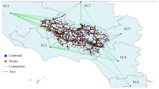
Figure 2.
Transport network diagram of the case study.
The total extension of the arcs (considering that all of them have been duplicated to represent two-way carriageways) is 4870 km.
The representation of the basic network graph can be observed in Figure 2.
From OpenStreetMap, the arcs of the road network are characterised by having several properties, including the most important, the C0, that is the maximum vehicle flow rate under prevailing traffic conditions, assigned on the basis of the type of road and of road cross-section layout, and the V0, that is a vehicle speed assuming a null vehicular density on that specific road arc. Both C0 and V0 are used in Equations (6) and (7).
The following figures show the distribution of C0 capacities (see Figure 3a) and undisturbed flow velocities V0 (see Figure 3b) in proportion to the length of the links.
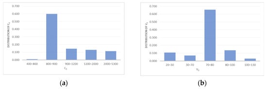
Figure 3.
(a) V0 speed distribution, (b) C0 capacity distribution.
Along the network, 208 bridges are present. All of them have been visually inspected and for each of them, a report has been filled, identifying maintenance and structural defects, according to the level 1 of recent Italian guidelines for the risk classification of existing bridges [36].
The main types of bridges present in the stock are as follows:
- Masonry bridge 2%;
- Reinforced concrete bridge 59%;
- Pre-stressed concrete bridge 30%;
- Steel–concrete bridge 9%.
4.1. Damage Scenarios
In order to assess the consequence of the bridge performance in the occasion of a seismic event, several damage scenarios have been generated. In this research, a single seismic event has been adopted for all the scenarios.
In each damage scenario, for all the bridges, the predicted ground motion intensities at site have been retrieved using a ShakeMap, and the damage states have been sampled, considering the probability provided by the fragility curves as a function of the ground motion intensity registered at the site of each bridge.
A number of 30 scenarios has been arbitrarily decided, since it was deemed statistically consistent with the initial assumptions about the seismic intensity and variability of damage pattern over the bridge stock. This choice will be discussed when presenting the results of the analysis.
The seismic event chosen for this study is the M 6.7 1349 earthquake, that occurred on 9 September 1349, in the south–west area of central Italy. This event is one of the most catastrophic events experienced along the Apennines, striking a vast area across Molise, Latium and Abruzzi, and whose effects were felt at a very large distance. [37,38]
The simulated ShakeMap for this event has been produced by INGV [39,40] and released for planning emergency response exercises. The ShakeMap event has been superimposed over the road network as shown in Figure 4, where the assumed epicentre position is depicted together with the contour lines expressing the ordinate of the acceleration spectrum Sa at a natural period of Tn = 1.0 s (SA1.0).
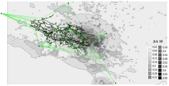
Figure 4.
ShakeMap of the case study (the red star represents the epicentre of earthquake) superimposed to the road network (see legend of Figure 2 for explanation of symbols).
The selection of the intensity measure to be adopted in a seismic risk analysis is a crucial step that should be consistent with the expected seismic performance of the class of structures to be studied and the vulnerability model adopted for the damage assessment. In this case, the choice has fallen on SA1.0, since the acceleration spectrum at a period very close to the natural one of the studied bridges has been proven to provide an unbiased damage estimate and to reduce the dispersion of the results [41,42,43]. A possible alternate solution could have been the peak ground acceleration (PGA) [44].
For the sake of simplicity and also in order to not disclose real data about critical infrastructural assets, only one set of fragility curves has been adopted in this study, not considering the specificity of the considered bridges. In particular, the study uses the fragility functions derived in [45]. As already pointed out in previous studies [4,12,14], those curves, originally conceived for the bridges serving the Greater Lisbon area, are also suitable to represent the vulnerability of the bridge stock in the central Italian investigated area. There are five damage states considered, as indicated in Table 2. The outcomes of the damage states sampled for the different damage scenarios are represented in Figure 5 (in average, only 5% of the bridges reach the collapse state, DS4, whilst 84% of them remain undamaged, DS0).

Table 2.
Capacity reduction based on the damage state of bridges.
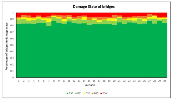
Figure 5.
Percentage of bridges in damage state.
The actual practicability of bridges in post-seismic conditions are conditioned by different factors, such as: the level of damage sustained, the works required for their repair/replacement and the traffic restrictions imposed by the regulatory authorities [46,47,48]. In this study, on the basis of the bridge damage state, the traffic capacity is reduced using a capacity reduction coefficient, αred, as follows:
where: Cact is the actual traffic capacity to be considered for the damaged bridges in the traffic assignment algorithms in Equation (5), C0 is the traffic capacity of the undamaged bridges and αrid is given in Table 2. The reduction factors in the table considers also the residual flow capacity that may be provided by local detour routes not directly included in the modelled network.
4.2. Zoning, Preliminary Traffic Flow Analysis and O/D Matrix
For this analysis, the study area coincides with the entire provincial territory.
Everything outside the border, called cordon, is the external environment and only interconnections with the study area are taken into account.
Generally, trips that are made in a given area can begin and end anywhere in the territory, but to allow the modelling of the transport system, it is necessary to discretise the study area in traffic zones, characterised by a centroid, where it is assumed that all the issued and attracted trips are located.
Taking into account the location of the inhabited area and the productive activities, and considering the results obtained from the preliminary analysis of the travels, a zoning with 91 internal zones and six external centroids was proposed and is presented in Figure 6.
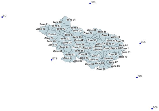
Figure 6.
Zoning of the study area.
With the aim of conducting a preliminary analysis of the traffic flows involving the study area and the relative construction of the O/D matrix, the traveling data relating to the aforementioned municipalities have been extrapolated from the commuting matrix.
This matrix, taken from the 15th General Population Census (9 October 2011), is edited every ten years by the Italian National Institute of Statistics ISTAT [30,31] and the analysed record layout contains information relating to home–work and home–study movements relating to the resident population.
In particular, the data used for this study contain the following information: the province of residence, municipality of residence, reason for travel (school or work), habitual municipality of study or work, departure time (before 7:15; from 7:15 to 8:15; from 8:15 to 9:15 and after 9:15), duration of traveling (>60 min; 30–60 min; 15–30 min and <15 min) and used mean of transport. Although 12 categories of the means of locomotion are present in the standard record, only car and bus have been selected in this study.
As extensively described previously, the O/D matrix is composed of four sub-matrixes, which require a separate preliminary analysis of the flows: internal trips to the province (II, Figure 1); external–internal trips (EI, Figure 1); internal –external trips (IE, Figure 1) and through trips (EE, Figure 1). The four preliminary analyses carried out are described separately below.
As far as internal trips are concerned, II, all the movements that took place between the various municipalities present in the provincial territory have been considered (excluding the internal movements of each individual municipality). Observing Table 3, the busiest time slot, and therefore chosen for the analysis, is from 7:15 to 8:15.

Table 3.
Percentage of internal journeys divided into various departure times (in bold typeface the selected solution for the analysis).
With regard to internal–external and external–internal trips, from the analysis carried out in the four time slots for cars and buses, it was found that six provinces account for more than 97% of the total trips issued and attracted by the provincial territory (see Table 4). For this reason, six external centroids are fixed, which represent the six identified provinces.

Table 4.
Percentage of internal–external (IE) and external–internal (EI) trips divided into the various provinces.
The departure time selected for internal–external trips is still between 7:15 and 8:15, as these flows, added to the internal ones, constitute the greatest traffic load on the transport network.
On the other hand, with regard to the selection of the departure time for external–internal trips, it is also necessary to consider the duration of these trips. In fact, in order to be able to load the road network in the time slot 7:15–8:15, starting outside of the provincial territory, trips must start before 7:15 and last at least 30 min. Table 5a,b summarise the percentages of external–internal trips, broken down into the various departure times and by trip duration, respectively.

Table 5.
(a) Percentage of external–internal (EI) trips divided into the various departure times (in bold typeface the selected solution for the analysis). (b) Percentage of external–internal (EI) trips broken down by trip duration.
Finally, with regard to the through trips, as a design choice, the six provinces that most interact with the provincial territory in terms of attracted and emitted trips have been selected. Furthermore, they constitute the cordon, which delimits the province in question (see Figure 2), and it is plausible to assert that they use the infrastructures present in this territory to reach each other. In particular, the combinations considered are summarised in Table 6.

Table 6.
Crossing trip combinations between external centroids (EC1–EC6 see Figure 2). The x symbol signifies that a combination exists.
Finally, observing Table 7a,b, which summarises the percentages of crossing trips broken down into the various departure times and trip duration, respectively, it is possible to deduce that, similarly to what was deduced for external–internal trips, the trips emitted first for 7:15 will be used for the crossing trips (EE) in the O/D matrix.

Table 7.
(a) Percentage of crossing trips (EE) divided into the various departure times (in bold typeface the selected solution for the analysis). (b) Percentage of crossing trips (EE) broken down by trip duration.
Having deduced these flows, it was possible to create the O/D matrix in which corrective coefficients were applied for the collective trips (busses) and it was also amplified to take into account trips for other reasons other than work and study.
4.3. Traffic Model Calibration
The traffic model calibration is essential to ensure that traffic demand was as close to reality as possible.
In particular, in the study, the measured flows provided by eighty automatic detection stations along the studied network were used. These stations ensure the automatic detection of vehicle flows through the use of magnetic sensors or toll-ticketing systems, without the presence of operators.
In a first phase of assignment (see Figure 7a), it can be noticed that there is no alignment between simulated flows and measured flows, obtaining a Pearson coefficient equal to 0.80.
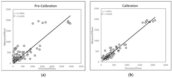
Figure 7.
(a) Pre-calibration between measured and simulated flows, (b) calibration between measured and simulated flows.
The calibration of the O/D matrix derived from ISTAT data [30,31] by counting network traffic was therefore carried out (see Figure 7b).
From the coefficient of Pearson pairs of 0.97, in Figure 7b, a good calibration is deduced between the estimated flows from the simulation and those measured; therefore, the model is very close to the real situation.
Below are the results of a typical day in the peak-hour early morning time slot in terms of vehicular flows assigned to the examined road network (see Figure 8).
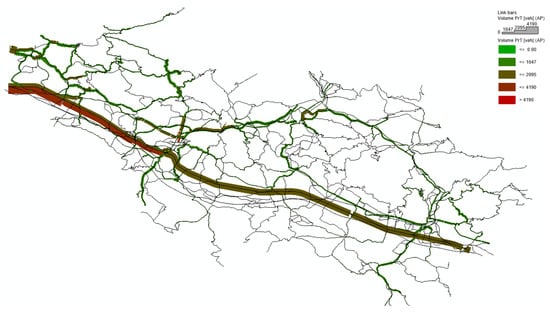
Figure 8.
Car and motorcycle mode traffic flow assignment for morning peak-hour matrix.
5. Discussion of Results
Following the calibration, it was possible to simulate the ex-ante scenario with the software Visum [19] and see the distribution of the ratio of volume and capacity by identifying congestion zones as in Figure 9.
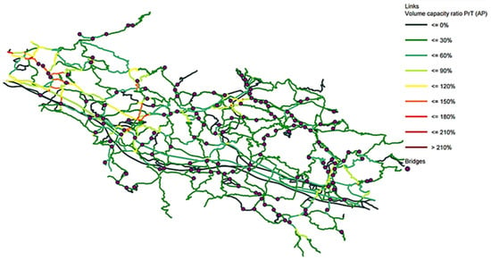
Figure 9.
Saturation of the ex-ante scenario.
As a result, by reducing the capacity according to the limit state assigned to the bridges (Equation (8)), it was possible to simulate a post-earthquake scenario (Equations (6) and (7)) with the following results in Figure 10.
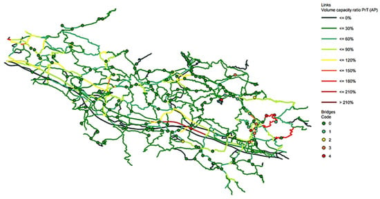
Figure 10.
Saturation of the ex-post scenario and the damage state of bridges.
In scenario 1 presented in Figure 10, bridges are characterised by the damage states (DM) indicated in Table 8.

Table 8.
Damage state of bridges in Scenario 1.
What can be noted is that in the post-earthquake scenario, the arches that are most congested are those at the bridges affected by high-damage states.
In particular, the motorway bridge that is in a limit state 4 leads to the closure of the motorway section concerned and a consequent congestion on possible alternative routes.
The same applies to the arches near the epicentre, where the bridges are in damage state 4.
What can be seen in comparison between the two scenarios is that the situations of a worsening saturation remain almost localised and do not spread over a wide range.
As for the times, the travel time matrices have been extrapolated in the situations before and after the earthquake.
Downstream of the generic scenario k, the matrix T(k) is obtained (of the same size as O/D), containing the travel times from i to j for the scenario k, derived from the matrix ΔT (delays), which is like O/D where each pair is i j.
where
- Tij(k) is estimated travel times in the ex-post k scenario;
- Tij(0) is estimated travel times in the ex-ante 0 scenario.
For each source–destination pair, a weighted average between the input and output flows multiplied by the relative delays recorded has been evaluated obtaining, for each centroid (i), the indicator :
where
- is the flow from centroid i to centroid j;
- is the flow from centroid j to centroid i;
- is the delay recorded from centroid i to centroid j;
- is the delay recorded from centroid j to centroid i.
These values were divided by the maximum delay in order to obtain a dimensionless indicator for each traffic area as presented in Figure 11.
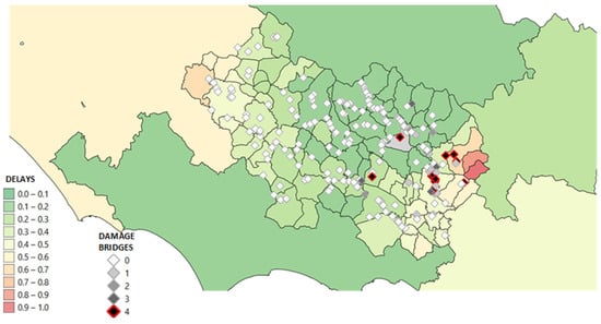
Figure 11.
Distribution of delays.
As can be seen from the figure, the internal traffic areas that are most affected by the effects of the earthquake are those closest to the bridges with DM4, DM3 and DM2.
The external traffic zones are strongly affected by this earthquake, since the loss of the service of a motorway bridge significantly increases the journey times of all the crossing movements.
Moreover, for municipalities with slightly damaged bridges but with significant delays, this is probably due to their high attractiveness.
In order to validate the model, 30 different scenarios have been implemented, all based on the same earthquake but with different bridges damaged.
An overall indicator has been evaluated indicating the ratio of travel times in the ex-post scenario (k) to travel times in the ex-ante scenario (0), both multiplied by flows.
These terms have the same meaning as those in (10).
The trend of the mean and the standard deviation of were evaluated in order to understand if 30 scenarios were sufficient to study this phenomenon.
Figure 12 below shows the average trend for delays in the 30 scenarios developed.
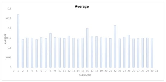
Figure 12.
Average of delays.
As can be seen from the graph in Figure 12, Scenario 1 is the one that deviates the most from the overall trend because in it, there are two very impacting conditions:
- -
- DM4 damage state bridge on a highway;
- -
- The isolation of a centroid.
Further deviations from the overall performance can be noted for Scenarios 8, 16 and 22, where one of the following conditions occurs:
- -
- DM3 or DM4 damage state bridge on a highway;
- -
- The isolation of a centroid.
In order to better understand if the amount of scenarios implemented allowed a stabilisation of the average, the trend of the progressive average expressed by Equation (12) was evaluated.
where:
- k is the number of scenarios included in the calculation.
As evidenced in Figure 13 as well as in Figure 14, it is possible to notice a deviation from the general course for the Scenarios 1, 8, 16 and 22.
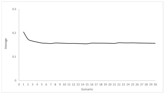
Figure 13.
Average of overall indicator .
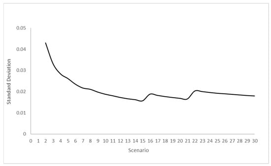
Figure 14.
Standard deviation of overall indicator .
From both, it is clear that a stabilisation is already obtained around the tenth scenario. Therefore, the number of scenarios chosen for this case study is more than sufficient.
The same calculation is repeated for the standard deviation (Figure 14), which is also evaluated progressively:
where:
- is the mean as calculated by Equation (12);
- is the number of scenarios included in the calculation.
6. Conclusions
The research presents a risk assessment of a realistic medium-sized road system after a major earthquake, considering possible bridge damage/collapse. A road network of the affected area has been constructed, including a realistic travel demand model. A main limitation of the study is that the developed O/D matrix is representative of the non-seismic conditions, despite the fact that it is widely recognised that after a severe earthquake like the one considered in this study, the damages to the built-environment may cause a general relocation of people and businesses, thus altering the initial assumptions of the travel demand adopted in the traffic model.
The methodology, given a seismic event, foresees the use of different damage scenarios in order to consider uncertainty in the structural vulnerability. By performing a traffic assignment in post seismic conditions over the network with damaged bridges, it was possible to identify the losses, in terms of time, that users suffer as a result of the seismic event. Global indicators have been proposed, representing the overall delay for all the users of the network.
The number of damage scenarios to be generated for an affordable estimate of those indicators is very limited.
From the study carried out, it is clear that an acceptable approximation value is already obtained from the first scenario, and therefore, the expected number, 30, is more than sufficient.
In particular, via analysing the results obtained in terms of trip duration, it was found that the greatest delays are observed in the close vicinity of the bridges sustaining a more severe damage, but also that those delays spread over a wider portion of the network when damaged bridges interfere heavily trafficked roads (such as highways).
Moreover, the network redundancy is a crucial aspect. Where alternative routes are absent, the traffic analysis reveals that centroid isolation is impossible for internal or external trips.
The results of this study can provide a reliable representation of the possible consequences of a seismic event and therefore permit to adopt the more appropriate mitigation strategies.
Author Contributions
Conceptualisation, A.R. and M.DA.; methodology, A.R. and M.D.; software, S.N. and A.E.; validation, S.N. and A.E.; formal analysis, S.N.; investigation, A.E. and M.D.; resources, A.R.; data curation, S.N. and A.E.; writing—original draft preparation, A.R., S.N. and A.E.; writing—review and editing, A.R., S.N., A.E. and M.D.; visualisation, S.N.; supervision, A.R. and M.D.; project administration, A.R.; funding acquisition, A.R. All authors have read and agreed to the published version of the manuscript.
Funding
This research received no external funding.
Data Availability Statement
The data used in this study appear in the submitted article.
Acknowledgments
The first author acknowledges the participation to the Research Project FIRMITAS (multi-hazard assessment, control and retroFIt of bridges for enhanced robustness using Smart Industrialised Solutions), financed by the Ministry of University and Research within the PRIN 2020 Programme (Grant No. 020P5572N_005) and to the CSLLPP/ReLUIS agreement: testing of guidelines for risk classification and management, safety assessment and monitoring of existing bridges, funded by the Ministry of Infrastructure.
Conflicts of Interest
The authors declare no conflict of interest.
References
- Nuti, C.; Rasulo, A.; Vanzi, I. Seismic safety evaluation of electric power supply at urban level. Earthq. Eng. Struct. Dyn. 2007, 36, 245–263. [Google Scholar] [CrossRef]
- Nuti, C.; Rasulo, A.; Vanzi, I. Seismic safety of network structures and infrastructures. Struct. Infrastruct. Eng. Maint. Manag. Life-Cycl. 2010, 6, 95–110. [Google Scholar] [CrossRef]
- Malekloo, A.; Ozer, E.; Ramadan, W. Bridge Network Seismic Risk Assessment Using ShakeMap/HAZUS with Dynamic Traffic Modeling. Infrastructures 2022, 7, 131. [Google Scholar] [CrossRef]
- Rasulo, A.; Pelle, A.; Briseghella, B.; Nuti, C. A Resilience-Based Model for the Seismic Assessment of the Functionality of Road Networks Affected by Bridge Damage and Restoration. Infrastructures 2021, 6, 112. [Google Scholar] [CrossRef]
- Nicolosi, V.; Augeri, M.; D’Apuzzo, M.; Evangelisti, A.; Santilli, D. A Probabilistic Approach to the Evaluation of Seismic Resilience in Road Asset Management. Int. J. Disaster Risk Sci. 2022, 13, 114–124. [Google Scholar] [CrossRef]
- D’Apuzzo, M.; Evangelisti, A.; Nicolosi, V.; Santilli, D.; Modoni, G.; Spacagna, R.L.; Paolella, L. Simplified approach for liquefaction risk assessment of transportation systems: Preliminary outcomes. In Computational Science and Its Applications—ICCSA 2020; Lecture Notes in Computer Science; Gervasi, O., Murgante, B., Misra, S., Garau, C., Blečić, I., Taniar, D., Apduhan, B.O., Rocha, A.M.A.C., Tarantino, E., Torre, C.M., et al., Eds.; Springer: Cham, Switzerland, 2020; Volume VII, pp. 130–145. [Google Scholar] [CrossRef]
- D’Apuzzo, M.; Evangelisti, A.; Spacagna, R.L.; Cappelli, G.; Nicolosi, V.; Modoni, G.; Paolella, L. Seismic Resilience Assessment Strategy for Social and Sustainability Impact Evaluation on Transportation Road Network: A Seismic Liquefaction-Induced Damage Application. Sustainability 2022, 14, 8411. [Google Scholar] [CrossRef]
- D’Apuzzo, M.; Evangelisti, A.; Spacagna, R.L.; Cappelli, G.; Nicolosi, V.; Paolella, L. Transportation infrastructures exposed to seismic risk: Evaluation of social costs for resilience design. In Computational Science and Its Applications—ICCSA 2023; Lecture Notes in Computer Science; Gervasi, O., Murgante, B., Misra, S., Garau, C., Blečić, I., Taniar, D., Apduhan, B.O., Rocha, A.M.A.C., Tarantino, E., Torre, C.M., et al., Eds.; Springer: Cham, Switzerland, 2023; in press. [Google Scholar]
- Kilanitis, I.; Sextos, A. Impact of earthquake-induced bridge damage and time evolving traffic demand on the road network resilience. J. Traffic Transp. Eng. 2019, 6, 35–48. [Google Scholar] [CrossRef]
- Kilanitis, I.; Sextos, A. Integrated seismic risk and resilience assessment of roadway networks in earthquake prone areas. Bull. Earthq. Eng. 2019, 17, 181–210. [Google Scholar] [CrossRef]
- Abarcaa, A.; Monteiroa, R.; O’Reillya, G.J. Simplified Indirect Loss Characterization for the Seismic Risk Assessment of Roadway Bridge Networks. Int. J. Disaster Risk Reduct. 2022, 74, 102948. [Google Scholar] [CrossRef]
- D’Apuzzo, M.; Evangelisti, A.; Nicolosi, V.; Rasulo, A.; Santilli, D.; Zullo, M. A Simplified Approach for the Prioritization of Bridge Stock Seismic Retrofitting. In Proceedings of the 29th European Safety and Reliability Conference (ESREL), Hannover, Germany, 22–26 September 2019; pp. 3277–3284. [Google Scholar]
- Abarca, A.; Monteiro, R.; O’Reilly, G.J. Seismic risk prioritisation schemes for reinforced concrete bridge portfolios. Struct. Infrastruct. Eng. 2023, 1–21. [Google Scholar] [CrossRef]
- D’Apuzzo, M.; Evangelisti, A.; Rasulo, A.; Nicolosi, V. Simplified approach to integrate seismic retrofitting prioritization with social cost evaluation: A case study in central Italy. J. Traffic Transp. Eng. 2022, 9, 447–460. [Google Scholar] [CrossRef]
- Maffei, J.R. Management and prioritization of bridge seismic evaluations and upgrading. In National Seismic Conference on Bridges and Highways; Progress in Research and Practice: San Diego, CA, USA, 1995. [Google Scholar]
- Nuti, C.; Vanzi, I. Screening of bridges for assessment and retrofit. In Seismic Bridge Design and Retrofit Structural Solutions: State-of-the-Art Report, Bulletin 39; Fédération Internationale du Béton: Lausanne, Switzerland, 2007. [Google Scholar]
- Gidaris, I.; Padgett, J.E.; Barbosa, A.R.; Chen, S.; Cox, D.; Webb, B.; Cerato, A. Multiple-hazard fragility and restoration models of highway bridges for regional risk and resilience assessment in the United States: State-of-the-art review. J. Struct. Eng. 2017, 143, 04016188. [Google Scholar] [CrossRef]
- El-Maissi, A.M.; Argyroudis, S.A.; Nazri, F.M. Seismic Vulnerability Assessment Methodologies for Roadway Assets and Networks: A State-of-the-Art Review. Sustainability 2021, 13, 61. [Google Scholar] [CrossRef]
- PTV Planung Transport Verkehr AG. Visum 17 User Manual; PTV AG: Karlsruhe, Germany, 2017. [Google Scholar]
- QGIS Development Team. QGIS Geographic Information System. Open Source Geospatial Foundation Project. 2017. Available online: http://qgis.osgeo.org (accessed on 18 April 2023).
- Esposito, T.; Mauro, R. La Progettazione Funzionale Delle Strade, Fondamenti di Infrastrutture Viarie, 1st ed.; Hevelius Edizioni srl: Benevento, Italy, 2003; Volume 2. [Google Scholar]
- National Research Council (NRC); Transportation Research Board (TRB). Highway Capacity Manual HCM 2000; NRC: Washington, DC, USA, 2000. [Google Scholar]
- Worden, C.B.; Wald, D.J. ShakeMap Manual Online: Technical Manual, User’s Guide, and Software Guide, U.S. Geological Survey. 2016. Available online: https://cbworden.github.io/shakemap/ (accessed on 6 June 2023). [CrossRef]
- Rasulo, A.; Goretti, A.; Nuti, C. Performance of lifelines during the 2002 Molise, Italy, earthquake. Earthq. Spectra 2004, 20, 301–314. [Google Scholar] [CrossRef]
- Rasulo, A.; Pelle, A.; Lavorato, D.; Fiorentino, G.; Nuti, C.; Briseghella, B. Finite Element Analysis of Reinforced Concrete Bridge Piers including a Flexure-Shear Interaction Model. Appl. Sci. 2020, 10, 2209. [Google Scholar] [CrossRef]
- Ferrari, P. Fondamenti di Pianificazione dei Trasporti; Pitagora Editrice: Bologna, Italy, 2001. [Google Scholar]
- Cascetta, E. Teoria e Metodi Dell’ingegneria dei Sistemi di Trasporto; Utet: Torino, Italy, 1998. [Google Scholar]
- Cascetta, E. Modelli per i Sistemi di Trasporto. Teoria ed Applicazioni; Utet: Torino, Italy, 2006. [Google Scholar]
- Cascetta, E. Transportation Systems Analysis, Springer Optimization and Its Applications 29; Springer: New York, NY, USA, 2009. [Google Scholar]
- Italian Institute of Statistics (ISTAT). Permanent Census of Population and Housing; Istat: Roma, Italy, 2011; Available online: https://www.istat.it/en/censuses/population-and-housing (accessed on 20 February 2023).
- Italian Institute of Statistics (ISTAT). Movements for Study or Work Reasons according to the Permanent Population Census; Istat: Roma, Italy, 2011; Available online: http://dati-censimentoindustriaeservizi.istat.it/Index.aspx?lang=en&SubSessionId=286d23f3-7622-4e49-b2e0-e072592a33c3 (accessed on 20 February 2023).
- Lee, D.-H.; Nie, Y. Accelerating Strategies and Computational Studies of the Frank–Wolfe Algorithm for the Traffic Assignment Problem. Sage J. 2001, 1771, 97–105. [Google Scholar] [CrossRef]
- Zhang, J.; Liu, M.; Zhou, B. Hindawi Analytical Model for Travel Time-Based BPR Function with Demand Fluctuation and Capacity Degradation. Math. Probl. Eng. 2019, 2019, 5916479. [Google Scholar] [CrossRef]
- Schnabel, W.; Lohse, D. Grundlagen der Straßenverkehrstechnik und der Verkehrsplanung; Kirschbaum—Beuth: Berlin, Germany, 1997. (In German) [Google Scholar]
- Deile, B.; Lätzsch, L.; Lohse, D. Studie zur Verkehrsnetzberechung mit Ka-Pazitätsbeschränkung; Forschungsbericht, University of Transport Dresden: Dresden, Germany, 1973. (In German) [Google Scholar]
- Ministry of Infrastructure Decree, no. 578, 17/12/2020. Enforcement of the Guidelines on Risk Classification and Management, Safety Assessment and Monitoring of Existing Bridges [Adozione delle Linee Guida per la Gestione del Rischio dei Ponti Esistenti e per la Definizione di Requisiti ed Indicazioni Relativi al Sistema di Monitoraggio Dinamico]; Ministero delle Infrastrutture e dei Trasporti: Roma, Italy, 2020. (In Italian) [Google Scholar]
- Galli Paul, A.C.; Naso José, A. Unmasking the 1349 earthquake source (southern Italy): Paleoseismological and archaeoseismological indications from the Aquae Iuliae fault. J. Struct. Geol. 2008, 31, 128–131, 145. [Google Scholar] [CrossRef]
- Guidoboni, E.; Comastri, A.; Mariotti, D.; Ciuccarelli, C.; Bianchi, M.G. Ancient and Medieval Earthquakes in the Area of L’Aquila (Northwestern Abruzzo, Central Italy), A.D. 1-1500: A Critical Revision of the Historical and Archaeological Data. Bull. Seism. Soc. Am. 2012, 102, 1606. [Google Scholar] [CrossRef]
- Michelini, A.; Faenza, L.; Lauciani, V.; Malagnini, L. ShakeMap implementation in Italy. Seismol. Res. Lett. 2018, 79, 688–697. [Google Scholar] [CrossRef]
- Michelini, A.; Faenza, L.; Lanzano, G.; Lauciani, V.; Jozinović, D.; Puglia, R.; Luzi, L. The New ShakeMap in Italy: Progress and Advances in the Last 10 Yr. Seismol. Res. Lett. 2020, 91, 317–333. [Google Scholar] [CrossRef]
- Shome, N.; Cornell, C.A.; Bazzurro, P.; Carballo, J.E. Earthquakes, records and nonlinear responses. Earthq. Spectra 1998, 14, 469–500. [Google Scholar] [CrossRef]
- Luco, N.; Bazzurro, P. Does amplitude scaling of ground motion records result in biased nonlinear structural drift responses? Earthq. Eng. Struct. Dyn. 2007, 36, 1813–1835. [Google Scholar] [CrossRef]
- Luco, N.; Cornell, C.A. Structure-specific scalar intensity measures for near-source and ordinary earthquake ground motions. Earthq. Spectra 2007, 23, 357–392. [Google Scholar] [CrossRef]
- Padgett, J.E.; Nielson, B.G.; DesRoches, R. Selection of optimal intensity measures in probabilistic seismic demand models of highway bridge portfolios. Earthq. Eng. Struct. Dyn. 2008, 37, 711–725. [Google Scholar] [CrossRef]
- Azevedo, J.; Guerreiro, L.; Bento, R.; Lopes, M.; Proença, J. Seismic vulnerability of lifelines in the greater Lisbon area. Bull. Earthq. Eng. 2010, 8, 157–180. [Google Scholar] [CrossRef]
- Bocchini, P.; Frangopol, D.M. A stochastic computational framework for the joint transportation network fragility analysis and traffic flow distribution under extreme events. Probabilistic Eng. Mech. 2011, 26, 182–193. [Google Scholar] [CrossRef]
- Hu, Z.; Zhou, J.; Zhang, S.; He, S.; Yu, B.A. Restriction Analysis of Transport Policy for Bridges Using the Trajectory Data. J. Adv. Transp. 2020, 2020, 8880335. [Google Scholar] [CrossRef]
- Kameshwar, S.; Misra, S.; Padgett, J.E. Decision tree-based bridge restoration models for extreme event performance assessment of regional road networks. Struct. Infrastruct. Eng. 2020, 16, 431–451. [Google Scholar] [CrossRef]
Disclaimer/Publisher’s Note: The statements, opinions and data contained in all publications are solely those of the individual author(s) and contributor(s) and not of MDPI and/or the editor(s). MDPI and/or the editor(s) disclaim responsibility for any injury to people or property resulting from any ideas, methods, instructions or products referred to in the content. |
© 2023 by the authors. Licensee MDPI, Basel, Switzerland. This article is an open access article distributed under the terms and conditions of the Creative Commons Attribution (CC BY) license (https://creativecommons.org/licenses/by/4.0/).