Abstract
Structural health monitoring (SHM) is a non-destructive testing method that supports the condition assessment and lifetime estimation of civil infrastructure. Sensor faults may result in the loss of valuable data and erroneous structural condition assessments and lifetime estimations, in the worst case with structural damage remaining undetected. As a result, the concepts of fault diagnosis (FD) have been increasingly adopted by the SHM community. However, most FD concepts for SHM consider only single-fault occurrence, which may oversimplify actual fault occurrences in real-world SHM systems. This paper presents an adaptive FD approach for SHM systems that addresses simultaneous faults occurring in multiple sensors. The adaptive FD approach encompasses fault detection, isolation, and accommodation, and it builds upon analytical redundancy, which uses correlated data from multiple sensors of an SHM system. Specifically, faults are detected using the predictive capabilities of artificial neural network (ANN) models that leverage correlations within sensor data. Upon defining time instances of fault occurrences in the sensor data, faults are isolated by analyzing the moving average of individual sensor data around the time instances. For fault accommodation, the ANN models are adapted by removing faulty sensors and by using sensor data prior to the occurrence of faults to produce virtual outputs that substitute the faulty sensor data. The proposed adaptive FD approach is validated via two tests using sensor data recorded by an SHM system installed on a railway bridge. The results demonstrate that the proposed approach is capable of ensuring the accuracy, reliability, and performance of real-world SHM systems, in which faults in multiple sensors occur simultaneously.
1. Introduction
Structural health monitoring (SHM) is a non-destructive evaluation technique that uses monitoring data recorded by sensors (“sensor data”), aiming to assess the condition and to estimate the lifetime of civil infrastructure [1]. SHM is primarily motivated by the need for safety and cost efficiency in structural maintenance, since SHM systems allow for reduced maintenance costs and provide continuous information on structural conditions [2]. The main target group of SHM encompasses aging infrastructure, which, due to poor maintenance, has led to disasters, such as the collapse of the Morandi bridge in Genoa, Italy [3]. SHM can help prevent the complete failure of civil infrastructure by assisting maintenance activities through filling the gaps of periodic visual inspections. Therefore, several research endeavors are underway to integrate SHM systems into “new” approaches related to Industry 4.0 and the Internet of Things, in an attempt to bring SHM systems into engineering practice [4], including new, user-friendly modeling and design concepts [5].
However, the reliability and performance of SHM systems, besides the proper synchronization of sensors [6], depend on the accurate operation of the sensing equipment. Sensors in monitoring systems may experience faults, compromising the reliability and performance of SHM systems. Sensor faults may be caused by hardware or software malfunctions, power outages, environmental impacts, or signal interferences [7]. The most common sensor faults include bias, complete failure, complete failure with noise, gain, drift, and outliers [8]. If undetected, sensor faults may compromise the accuracy of the sensing equipment, resulting in the low reliability and poor performance of SHM systems.
Fault diagnosis (FD) approaches for monitoring systems, including SHM systems, have been proposed to detect, isolate, identify, and accommodate sensor faults [9]. FD for SHM systems has been based on either physical or analytical redundancy. Physical redundancy requires installing several sensors on civil infrastructure. Then, based on majority-voting logic, outputs of redundant sensors decide whether a sensor is faulty or non-faulty [10]. The high cost, power consumption, and maintenance required by physical redundancy approaches for FD have been the primary motivations for using analytical redundancy [11]. Analytical redundancy uses mathematical models to describe a system and takes advantage of the redundant information inherent in the sensor data. In analytical redundancy approaches, fault detection relies on residuals between sensor data and “virtual outputs” thereof, estimated by mathematical models [9]. The residuals are evaluated using threshold logic or hypothesis testing for fault detection [12].
A special class of mathematical model used for FD falls into the category of artificial intelligence (AI), motivated by the complex and, frequently, nonlinear relationships within sensor data. In this context, neural networks have been extensively used in FD for SHM. In [13], multilayer neural networks were used to detect faults in the mechanical components of wind turbines. Similarly, neural networks have also been used to evaluate and to assess SHM systems. In [11], artificial neural network (ANN) models were embedded into wireless sensor nodes to autonomously detect and isolate sensor faults in a decentralized manner. In [14], the approach proposed in [11] was extended from the time-domain to the frequency-domain for FD. Furthermore, a combination of ANN models and convolutional neural network models was reported in [15], in which ANN models were used for sensor fault detection, isolation, and accommodation, while convolutional neural networks performed fault identification. However, the previously mentioned analytical redundancy approaches for SHM have been limited to the diagnosis of sensor faults occurring in individual sensors at different times, thus limiting their application to real-world SHM systems, in which sensor faults in multiple sensors may occur at the same time (simultaneous sensor faults).
Simultaneous sensor faults have rarely been considered within the scope of SHM systems for civil infrastructure, but have been a matter of interest in other disciplines and applications, as will be presented in the following two paragraphs. In the chemical industry, for example, a state-observer design has been used to exploit analytical redundancy in a nonlinear process system, specifically a chemical reactor, to differentiate between and isolate simultaneous sensor and actuator faults [16]. Moreover, in [17], simultaneous sensor and actuator faults were addressed using a descriptor fuzzy sliding-model observer. In [18], a review of data-driven approaches for FD in chemical processes was carried out. The authors of the review pointed out that most of the data-driven approaches are application-specific, and simultaneous FD is still a challenge. In addition, in the context of simultaneous sensor and actuator faults, descriptor observers for control systems, tested on a simulation example have been suggested [19]. Sensors and actuator faults were also addressed in [20], focusing on signals in a finite-frequency domain, and simultaneous actuator faults of quadrotor unmanned aerial vehicles have been detected using adaptive fuzzy state estimators and an integral terminal sliding-model control [21]. Furthermore, simultaneous sensor and actuator faults for fixed-wing unmanned aerial vehicles were investigated using recurrent wavelet fuzzy neural networks and a fractional-order sliding-model control in [22], and a backstepping approach in [23]. In [24], simultaneous actuator and sensor faults as well as simultaneous faults in multiple sensors were detected and identified in a linear simulation of unmanned aerial vehicles, using a Kalman filter approach.
An analytical redundancy approach was proposed in [25] to detect and isolate faults of multiple sensors in heating, ventilation, and air conditioning systems, for which robustness and scalability were also have been investigated [26]. In [25], fault detection was realized by an adaptive threshold, based on differential-algebraic estimators and a reasoning-based logic for fault isolation. The approach has been extended to detect and isolate faults of multiple heterogeneous sensors of marine fuel engines [27]. Furthermore, the approach has been extended to consider multiple sequential or simultaneous sensor faults for a network of interconnected cyber-physical systems and large-scale interconnected nonlinear systems [28,29]. Principal component analysis (PCA) has been proposed for the detection, isolation, and accommodation of faults in multifunctional sensors, i.e., sensors that measure more than one parameter and are more prone to fail simultaneously [30]. The authors in [31] suggested adding artificial neural networks to PCA to detect multiple faults in the rotors and stators of industrial motors. A data-driven approach based on residuals for industrial controllers was investigated in [32] to accommodate multiple simultaneous sensor faults.
In summary, despite the large body of research conducted on FD in SHM in civil infrastructure, most approaches address sensor faults occurring in individual sensors [33], in which over a period of time only one sensor is faulty [7], and do not consider sensor faults occurring in multiple sensors simultaneously. Research in other disciplines, such as the chemical industry, and aviation and flight-control systems, have addressed simultaneous sensor faults, but studies addressing the monitoring of civil infrastructure have been scarce. Furthermore, FD studies for simultaneous sensor faults in real-world SHM systems, where noise, external effects, and different loading conditions may affect the performance of FD approaches, have also been limited. In addition, to the knowledge of the authors, FD approaches adapting to the new state of the SHM systems after detecting multiple sensor faults have not been proposed.
To extend FD in SHM towards simultaneous sensor faults in multiple sensors, this paper presents an adaptive FD approach based on analytical redundancy (AFDAR). The AFDAR approach builds upon previous work, in which artificial neural networks and signal processing was proposed for FD in SHM systems [11,15]. Therein, the sensor data of individual sensors was estimated using artificial neural networks, to which correlated sensor data from other, typically neighboring sensors were used as input data, addressing single-fault occurrence under the premise that the input data to each ANN is non-faulty. However, as multiple sensors in real-world SHM systems may exhibit faults simultaneously, ANN models will use data from faulty sensors as input data and, thus, contaminate the predictions. By contrast, the AFDAR approach proposed in this study combines ANN models with moving averages of individual sensor data to detect, isolate, and accommodate sensor faults in multiple sensors. Fault identification is not included in this work because it is independent from single-fault occurrence or multiple-fault occurrence and has been effectively addressed in previous work [15].
The remainder of the paper is structured as follows: Section 2 introduces the methodology of the AFDAR approach. Next, the implementation of the AFDAR approach is described in Section 3, including an algorithmic representation. In Section 4, two validation tests, using artificial and real-world faults, are performed with sensor data recorded from a SHM system installed on a railway bridge. The results of the validation tests are presented and discussed in Section 5. Finally, the work presented herein is summarized and an outlook on future work as well as potential improvements in the AFDAR approach are suggested.
2. Methodology of the AFDAR Approach
This section introduces the methodology of the AFDAR approach for fault detection, isolation, and accommodation. In particular, the ANN models and the moving average (MA) concept are briefly discussed.
The motivation behind using ANN models for fault detection lies in the capabilities of ANN models to combine complex relationships between sensor data to make predictions. Artificial neural networks are a class of algorithms that use parallel computational principles, inspired by biological nervous systems. The scope of artificial neural networks covers tasks that are difficult to solve with deterministic algorithms or classical physics-based models, for example nonlinear problems, such as the diagnosis of sensor faults [11]. To present the methodology of the AFDAR approach, the topology of an exemplary ANN model is shown in Figure 1. In general, each ANN model has an input layer, one or several hidden layers, and an output layer. The input layer encompasses the input neurons, to which input data are fed. Since the purpose of each ANN model is to predict the sensor data of a single sensor using correlated data from neighboring sensors (hereinafter termed “correlated sensors”), the sensor data from the correlated sensors are used as input data. Each hidden layer ℓ is formed by neurons that receive weighted combinations w of the outputs of neurons (“activations”) belonging to the preceding layer ℓ-1, to which the neurons of layer ℓ are connected via arrows, termed “synapses”. Each activation of layer ℓ is computed through an “activation function”, which is applied when the input of a neuron exceeds a threshold. The last hidden layer forwards its activations to the output layer, which yields the predictions of the ANN model, i.e., in this study, the virtual outputs of a single sensor.
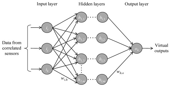
Figure 1.
An exemplary artificial neural network.
The AFDAR approach consists of four steps: (i) initialization, (ii) fault detection, (iii) fault isolation, and (iv) fault accommodation. The initialization step starts with investigating the correlations inherent in data recorded by sensors in the SHM system to find a set of correlated sensors. Thereafter, data from the set of correlated sensors are prepared to train the ANN models. In this context, and to avoid overfitting of ANN models, the data are divided into training data (70%), validation data (20%), and testing data (10%). During the training phase, the training data are fed into the ANN model, in which the model “learns” from existing relationships between known input data (sensor data from correlated sensors) and known output data (sensor data from the single sensor). Meanwhile, the validation data are used to evaluate the model performance during the training phase and tune the weights of connections between neurons in the ANN model. Upon completing the training phase of the ANN models, the testing data are used to evaluate the prediction capability of the ANN model with a different set of known input–output data, independent from the set used in the training phase.
The virtual outputs are compared with the sensor data from the single sensor, and if the residuals of the comparison lie below the fault detection threshold, the training is considered successful. Once the training has been successfully finished, fault detection is performed in the second step by feeding new input data into the input layers of the ANN models and producing new virtual outputs. The occurrence of faults is declared if the difference between the virtual outputs and the sensor data exceeds the fault detection threshold.
Fault isolation follows fault detection, i.e., the declaration of the occurrence of sensor faults as a result of the virtual outputs produced by the ANN models. A fault time stamp is utilized to specify a time window with length N, for which the moving average values of p data points uij (j = 1, …, p, p < N) are computed for sensor i (Equation (1)).
Gradual or abrupt changes in the values are indicative of faults. It should be noted that the reliability of the MA in isolating faults can only be ensured once the faults have been detected by the ANN models, and the corresponding fault time stamp has been established. In other words, bypassing the fault detection step and simply attempting to track changes in MA values of sensor data from individual sensors across the entire time period of monitoring may result in “false positives” because these changes may be attributed to fluctuations in the sensor data induced by variability in loading and/or environmental conditions affecting the structure being monitored by the SHM system.
Fault accommodation, the last step of the AFDAR approach, relies on the ability of the ANN models to adapt to the current state of the SHM system. As a result, the knowledge transferred from the fault isolation step is necessary for removing faulty sensors from the input layers of the ANN models to avoid contaminating the virtual outputs. Retraining the ANN models is accomplished by repeating the training phase, described previously, with sensor data prior to the fault time stamp. The implementation of the AFDAR approach is presented in the next section.
3. Implementation of the AFDAR Approach
The implementation of the proposed AFDAR approach in an SHM system is described in this section, referring to the four steps introduced above. A flowchart depicting the workflow of the AFDAR approach is shown in Figure 2. In what follows, the implementation of the four steps is briefly discussed.
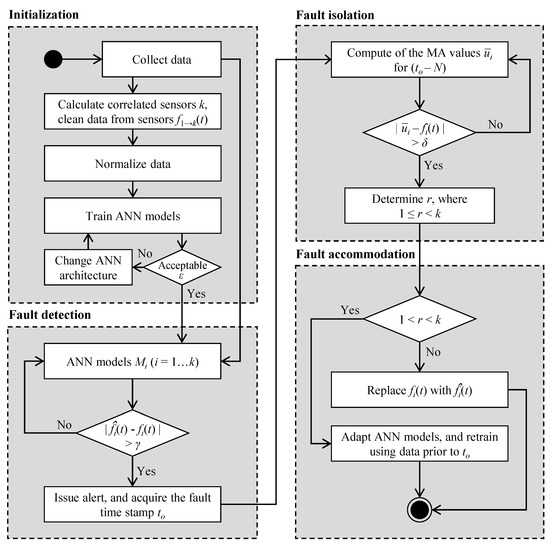
Figure 2.
Flowchart of the AFDAR approach.
- Initialization:
- To identify correlated sensors, data recorded by the sensors in the SHM system undergo a correlation analysis. The result of the correlation analysis determines the number of correlated sensors k. Then, data recorded by correlated sensors f1→k(t) is “cleaned”, i.e., if sensor data from an individual sensor are missing at a specific time window, the same time window is neglected in correlated sensors.
- The sensor data to be used for training the ANN models are normalized to avoid extremities in activations that would hinder the training process, using a minimum–maximum normalization, depicted in Equation (2), in which x denotes an arbitrary measurement in the sensor data, xmin and xmax are the minimum and maximum measurements in the sensor data, respectively, and xnormalized is the normalized value. The same normalization is applied to newly recorded sensor data that are fed to the ANN models after training.
- One ANN model Mi for each correlated sensor i (i = 1, …, k) is designed and trained using sensor data from the SHM system. During the training of Mi, sensor data from the correlated sensors (1, 2, …, i – 1, i + 1, …, k) are used as input data, and sensor data fi(t) from the sensor i are used as output data. As a result of the training, model Mi estimates the virtual outputs of sensor i, denoted by . The training phase of each ANN model involves selecting the ANN architecture, in terms of the number of hidden layers and number of neurons per hidden layer. An acceptable ANN architecture is based on the prediction accuracy of the model Mi lying below the fault detection threshold γ, determined by the root mean squared error (RMSE) value ε between the virtual outputs and the sensor data fi(t), as described in Equation (3). Upon completing the training of the ANN models, the models are deployed on a central computer of the SHM system to automatically detect, isolate, and accommodate sensor faults.
- Fault detection:
In this step, newly recorded sensor data are fed into all ANN models. In the event of faults occurring in r sensors (1 < r < k), the residuals between the actual sensor data and the virtual outputs in models Mn (n = 2, …, r) are expected to exceed γ, which, on the one hand, issues a fault detection alert only for the r sensors. The time to marking the violation of the fault detection threshold γ serves as the fault time stamp. On the other hand, the (faulty) sensor data fn(t) are also used as inputs to the s models Mv (v = 1, …, s, r + s = k) of the unfaulty sensors, which results in contaminating the virtual outputs of the Mv models and in yielding residual values that also exceed γ. Evidently, despite the design and training of ANN models dedicated for each correlated sensor, fault isolation requires further analysis of the sensor data on an individual sensor level. However, conducting the analysis on an individual sensor level requires the fault time stamp to, which represents the knowledge transferred to the next step.
- 3.
- Fault isolation:
- For fault isolation, the time window for the MA is defined around the fault time stamp to. The time window should have an adequate length N before the fault time stamp (to − N), to ensure the reliable tracking of the moving average.
- Equation (1) is applied to compute the MA across the entire length of the time window with a step of p data points of sensor i. Discrepancies between MA values and the fault isolation threshold δ from time to forward indicate the faulty sensor data of a sensor i.
- 4.
- Fault accommodation:
- 5.
- Once the fault isolation has been completed and the r faulty sensors have been specified, the ANN models adapt to the new conditions of the SHM system as follows:
- Adapting the ANN models essentially entails removing sensor data of the r correlated sensors that have been diagnosed as faulty from the ANN input layers of all models. As a result, the architectures of the ANN models are modified, and retraining the ANN models is necessary to produce virtual outputs for the faulty sensors.
- Retraining is achieved using sensor data prior to time to. Upon completing the retraining, the virtual outputs of the Mn (n = 2, …, r) models are used as substitutes for the faulty sensor data, thus accommodating the sensor faults.
The threshold γ is defined based on the maximum RMSE value (εmax) obtained during the training of the ANN models. The reasoning behind adopting the εmax value as threshold, instead, e.g., from the εmin of the training, is to grant each ANN model a somewhat conservative character, avoiding “false negative” outcomes in the fault detection step, i.e., neglecting potential faults that would result in RMSE values marginally higher than εmin. Furthermore, the fault isolation threshold δ is defined based on the accuracy of the sensors. Therefore, both thresholds γ and δ are case-specifically defined according to the application area. The validation of the AFDAR approach, using sensor data from a real-world SHM system is presented in the next section.
4. Validation of the AFDAR Approach
In this section, the AFDAR approach is validated via two tests using sensor data from a real-world SHM system installed on a railway bridge. In the first validation test, sensor faults were artificially injected into a clean dataset recorded by the SHM system. In the second validation test, the AFDAR approach was applied to a new dataset recorded by the SHM system over one year to diagnose real-world sensor faults. As a result, the proposed AFDAR approach was validated, ensuring the accuracy, reliability, and performance of real-world SHM systems in which faults in multiple sensors may occur simultaneously.
4.1. Description of the Railway Bridge and of the SHM System
The validation tests were conducted on a composite double-track railway bridge, located in Germany. The bridge consists of two parallel steel truss girders that support a 45 cm thick reinforced concrete (RC) slab. The bridge comprises 15 spans, each 58 m in length except for the edge spans, which are 57 m in length, and has a total length of 868 m. The deck width is 14.1 m, and the distance between the centroids of the steel truss girders is 6.2 m, as shown in the cross section of an inner span, illustrated in Figure 3.
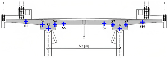
Figure 3.
Bridge cross-section and location of embedded temperature sensors (blue pluses).
A SHM system was installed on the bridge consisting of temperature sensors, displacement transducers, potentiometers, and strain gauges. In general, sensor faults have the same mechanisms and nature, regardless of the sensor type. In other words, deviations in sensor data from strain gauges, caused by drift, gain, bias or complete failure, follow the same patterns as deviations in sensor data from temperature sensors. As a result, for the sake of brevity and simplicity in the validation test, the sensor data from 10 temperature sensors were used, which were embedded in the RC slab in the positions depicted in Figure 3 (S1, …, S10). The temperature sensors were of type Pt100, measuring at a range from −35 °C to 105 °C with a sensitivity of ± 0.5°C. The sensor data recorded by the temperature sensors was transferred to a central computer, where it was processed and stored.
4.2. Description of the Validation Test
The temperature measurements used for validation were recorded over almost five years with a sampling rate of 1.7 mHz, i.e., one temperature measurement was recorded every 10 min, with a total of 256,000 measurements recorded by each sensor. In the initialization step, which is common for both validation tests, correlations between the temperature measurements recorded over a period of two years were investigated via correlation analysis. A strong positive correlation was unveiled by the Pearson correlation coefficient among all 10 temperature sensors belonging to the SHM system; hence, the number of correlated sensors was set to k = 10. The lowest correlation coefficient was 0.994 between sensors S2 and S5. Next, temperature measurements from the correlated sensors in the SHM system were cleaned and normalized to train the ANN models.
A total of 10 ANN models, equal to the number of correlated sensors (k = 10), were trained. Each model predicted the virtual outputs of one sensor, using temperature measurements from the other nine correlated sensors in the SHM system as input data. As a result, each ANN model had nine input neurons and one output neuron; the number of hidden layers and neurons per hidden layer was determined with different ANN architectures. Before training the ANN models for FD, the temperature measurements were split into training and testing sets. An ANN with a 9-32-64-256-256-1 architecture was determined for all ANN models, based on the lowest RMSE values ε, which lay between 0.09 and 0.15, with a total training time of approximately 680 s for each ANN model. The fault detection threshold was set to γ = 0.15, based upon engineering judgment. Exemplarily, Figure 4 illustrates the architecture of the ANN model M1, predicting the virtual outputs (t) for sensor S1 using temperature measurements from correlated sensors f2→10(t) as input data. With the training of the 10 ANN models, the initialization phase was completed, and the remaining steps of the AFDAR approach, i.e., fault detection, fault isolation and fault accommodation, were executed separately for each validation test.
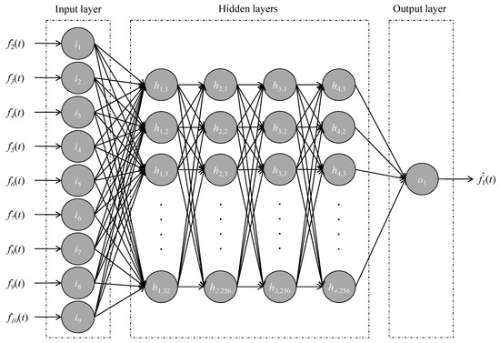
Figure 4.
Architecture of the ANN model for sensor 1.
In the first validation test, faults were artificially injected into a clean dataset. First, the dataset was manually inspected to confirm a clean and fault-free dataset, in which artificial faults could be injected. Then, under “controlled conditions”, i.e., with prior knowledge of the existence of faults, faults were artificially injected into the non-faulty set of temperature measurements to evaluate the ability of the proposed AFDAR approach. The injected faults included complete failure, complete failure with noise, outliers, drift, bias, and gain. Exemplary visual representations of the artificially injected faults are depicted in Figure 5. A total of 1717 faulty temperature measurements were injected simultaneously in multiple sensors.
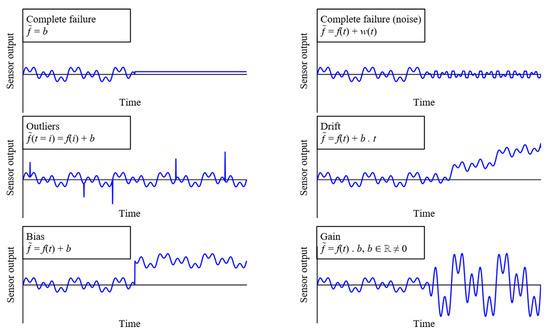
Figure 5.
Types of artificially injected sensor faults.
In the second validation test, the AFDAR approach was applied to new temperature measurements recorded by the SHM system. Unlike the first validation test, where faults were injected under controlled conditions, no prior knowledge was available about the correct or incorrect operation of the sensors that record the data in this case. Therefore, when faults were detected in the SHM data, the data from the faulty sensor was visualized side-by-side with the data from the correlated sensors. The reason for visualizing the data was to perceive deviations between the faulty sensors detected by the AFDAR approach and the correlated sensors. The results of the validation tests are presented and discussed in the next section.
5. Results and Discussion
In this section, the results of the AFDAR approach with faults artificially injected into the temperature measurements are shown, followed by the results of applying the AFDAR approach to a dataset that is newly recorded by the SHM system and contains real-world sensor faults.
5.1. Artificially Injected Faults
The results of applying the AFDAR approach on the temperature measurements recorded by the real-world SHM system with the artificially injected faults are shown in Table 1, expressed by the number of detected faults and the fault detection accuracy. The results show that 95.9% of the artificially injected faults are detected.

Table 1.
Fault detection results of artificially injected faults.
To describe the results of fault detection, isolation, and accommodation, the first row of Table 1, which addresses the simultaneous complete failure of sensors S1 and S2, was analyzed in more detail. Fault detection was positive when residuals between the temperature measurements of sensors S1 and S2 and the virtual outputs of models M1 and M2 exceeded the fault detection threshold of γ = 0.15. Next, a corresponding fault time stamp to = 101 min was recorded and transferred to the following AFDAR step, i.e., fault isolation, to isolate the faulty sensors. A time window with length of N = 25 min was utilized prior to the fault time stamp of to = 101 min, for which the MA was calculated individually for each sensor in the range of the correlated sensors (k = 10). At this point, it was still unknown which sensors were faulty. Then, if the residuals between the MA of each sensor and the recorded temperature measurement from to = 101 min onward exceeded the fault isolation threshold δ, the sensor was isolated. The value of the fault isolation threshold (δ) was set to the accuracy of the temperature sensors ± 0.5 °C. The MA value for the sensors S1 and S2 was 6.2 °C and 5.6 °C, respectively; however, no temperature measurements were recorded from to = 101 min onward. As a result, both sensors S1 and S2 were isolated.
In the final step, fault accommodation, temperature measurements recorded by the faulty sensors S1 and S2, f1(to ≥ 101) and f2(to ≥ 101), could not be replaced with the virtual outputs (to ≥ 101) and (to ≥ 101), respectively, because temperature measurements recorded by sensor S1 f1(to ≥ 101) were used as an input for model M2, which would result in the contamination of the virtual output (to ≥ 101), and vice versa. Consequently, both models M1 and M2 were adapted to this simultaneous fault by modifying the architecture of the ANN models M1 and M2. Thus, temperature measurements from S1 and S2 were shifted from the ANN input layer of models M1 and M2 to the output layer, and data prior to to = 101 min was used to train the adapted model M1,2. Figure 6 illustrates the architecture of the adapted ANN model, M1,2, predicting the virtual outputs and for both sensors, S1 and S2.
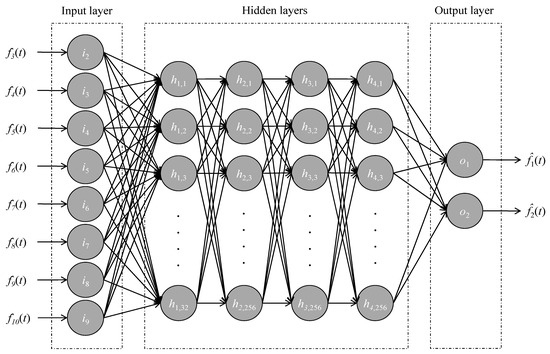
Figure 6.
Adapted model M1,2 for sensors S1 and S2.
Representing a case with more than two simultaneous faults, the fault detection step was activated in the time window 901–1000 min after residuals between the temperature measurements of sensors S3, S5, and S7 and the virtual outputs of the models M3, M5, and M7 exceeded the fault detection threshold of γ = 0.15. A fault time stamp of to = 901 min was recorded and transferred to the fault isolation step. Upon isolating the three faulty sensors, models M3, M5, and M7 were adapted to the three simultaneous faults in the fault accommodation step, and data prior to to = 901 min was used to train the adapted model M3,5,7, predicting virtual outputs , , and for sensors, S3, S5, and S7.
In Figure 7, a visual representation of the temperature measurements and the artificially injected faults are presented in Figure 7. Furthermore, in Figure 7, the results of applying the AFDAR approach are presented. As can be seen from Figure 7, the AFDAR approach has successfully achieved FD for sensor faults occurring simultaneously in multiple sensors of the SHM system. The continuous blue line represents the temperature measurements obtained by the sensors in the SHM system with the artificially injected sensor faults, the dashed green line shows the virtual outputs of the ANN models, and the dotted black lines represent the fault detection thresholds.
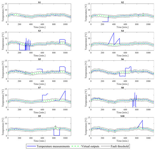
Figure 7.
Artificially injected faults detected by the AFDAR approach.
5.2. Real-World Sensor Faults
The results of applying the AFDAR approach with temperature measurements newly recorded by the SHM system are presented herein. The temperature measurements used in this validation test correspond to a period of one year; specifically, 52,560 temperature measurements were recorded by each sensor. Table 2 introduces the number of faults diagnosed by the AFDAR approach in the newly recorded data.

Table 2.
Real-world sensor faults detected by the AFDAR approach.
As shown in Table 2, the AFDAR approach has diagnosed 4632 faults in the new data recorded over one year. To ensure that the proposed AFDAR approach correctly detected real-world sensor faults, and since data were recorded by the same type of sensors (temperature sensors), the data recorded by all temperature sensors were visualized side-by-side. By visualizing and comparing the data, deviations in the faulty sensor data can be observed. Figure 8 shows the data recorded by the correlated sensors in the SHM system. In the figure, the continuous red line represents the data recorded by sensor S3, the continuous green line represents data recorded by sensor S8, and the dotted lines show data recorded by the correlated sensors in the SHM system.
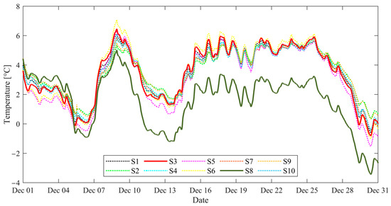
Figure 8.
Comparison of temperature measurements recorded by the ten temperature sensors of the SHM system.
As depicted in Figure 8, from December 5, data recorded by sensor S8, represented with the green continuous line, started deviating from the data recorded by the other sensors. The deviation in the data recorded by sensor S8 may be attributed to a drift occurring in the sensor. Furthermore, in the figure, between December 19 and December 20, no data were recorded by sensor S3, which may be attributed to a complete failure of the sensor.
The faults occurring simultaneously in sensors S3 and S8 were detected by the AFDAR approach, as the recorded temperature measurements exceeded the fault detection threshold, as shown in Figure 9. The figure shows data recorded by sensors S3 (top, continuous red line) and S8 (bottom, continuous green line). The dashed green line shows the virtual outputs of the ANN models, and the dotted black lines represent the fault detection thresholds. It should be noted that a total of 274 simultaneous faults occurred in sensors S3 and S8 between December 19 and December 20; however, the focus was drawn only on simultaneous faults that occurred in the aforementioned period, which fall within the scope of this paper.
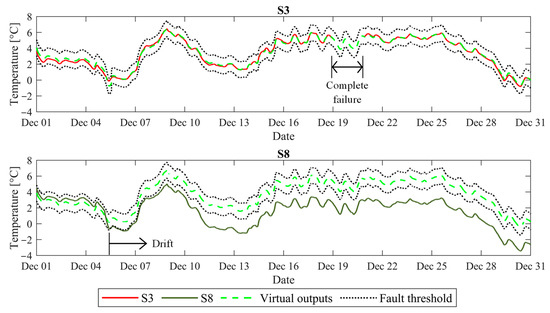
Figure 9.
Comparison of temperature measurements and virtual outputs with the fault threshold.
To describe the results of the fault detection, isolation, and accommodation for simultaneous real-world sensor faults, sensors S3 and S8 between December 19 and December 20 were analyzed in more detail. Similar to the previous validation test, fault detection was performed when residuals between the recorded temperature measurements from sensors S3 and S8, and the virtual outputs of models M3 and M8, exceeded the fault detection threshold of γ = 0.15. Then, fault isolation was conducted using the fault time stamp to of simultaneous fault occurrence in both sensors S3 and S8, which was determined at to = 01:20, on December 19. First, the fault isolation threshold was set to the accuracy of the temperature sensors ± 0.5 [°C]. Then, observing that the residuals between the MA values of sensors S3 and S8 and the respective temperature measurements at to exceeded the fault isolation threshold δ, the faulty sensors were isolated. Finally, fault accommodation was performed: Since both sensors S3 and S8 were faulty, models M3 and M8 were adapted by modifying the architecture of the ANN models. The ANN architecture was modified by shifting sensors S3 and S8 from the input layer to the output layer, and data prior to to were used to train the adapted ANN model M3,8. Figure 10 illustrates the architecture of the adapted ANN model M3,8, predicting the virtual outputs and for both sensors S3 and S8.

Figure 10.
Adapted model M3,8 for sensors S3 and S8.
6. Summary and Conclusions
Sensor fault diagnosis concepts have been increasingly adopted by the SHM community because sensor faults may significantly disrupt monitoring strategies. Contrary to sophisticated FD approaches in several disciplines addressing complex scenarios with multiple sensor faults, FD approaches for SHM have typically considered single-fault occurrence, which may underestimate the risks posed by sensor faults in real-world SHM systems. To extend FD to SHM by covering the occurrence of simultaneous sensor faults in multiple sensors, this paper has presented the AFDAR approach, an adaptive FD approach for simultaneous sensor faults in SHM systems, based on analytical redundancy. The AFDAR approach combines ANN models with moving averages of individual sensor data (i) to detect, (ii) to isolate, and (iii) to accommodate sensor faults in multiple sensors. Fault identification, commonly regarded as another step within fault diagnosis, has not been included within the scope of the AFDAR approach, because the identification of faults is independent from single-fault occurrence or multiple-fault occurrence and has been effectively addressed in previous work. Fault detection is achieved with ANN models, which predict virtual outputs for each sensor of an SHM system, on the basis of comparison between the virtual outputs and actual measurements. Then, the faults are isolated by comparing the moving average of the sensor data around the time instance of fault detection, individually for each sensor, with the fault isolation threshold. Finally, fault accommodation is conducted by replacing faulty data from sensors with the virtual outputs predicted by the ANN models upon adapting the models by removing faulty sensor data from the input neurons. As opposed to other analytical redundancy approaches that have been reported for SHM, the AFDAR approach considers multiple sensor faults occurring simultaneously.
To validate the AFDAR approach, two validation tests have been conducted. In the first validation test, artificial sensor faults were injected into a dataset containing sensor data recorded by a real-world SHM system installed on a composite (i.e., steel truss and reinforced concrete slab) railway bridge. In the second validation test, the proposed AFDAR was applied with sensor data newly collected by the SHM system to evaluate the ability to diagnose real-word sensor faults. The results achieved in the validation tests have confirmed the accuracy, reliability, and performance of the FD approach to detect, isolate, and accommodate sensor faults. Furthermore, the AFDAR approach has been proven capable of adapting to the new conditions of the SHM system regardless of the number of faulty sensors. In summary, the AFDAR approach can be used to ensure the accuracy of any type of sensors and thus ensure the reliability and performance of SHM systems installed on civil infrastructure.
In future research, the AFDAR approach may be extended and validated on damaged structures to investigate ways of differentiating between structural damage and sensor faults. Finally, the AFDAR approach may be distributedly implemented into wireless sensor nodes to automatically assess the condition of SHM systems on board the sensor nodes. Decentralizing the AFDAR approach into wireless sensor nodes, as opposed to transmitting all sensor data to central servers, is expected to decrease the energy spent on data communication, to reduce storage requirements, and to avoid the analysis of large amounts of raw data in central servers.
Author Contributions
All authors (T.A.-Z., C.C.G., K.D. and K.S.) contributed to the conception and design of the manuscript. The data curation, formal analysis, methodology, and software development was performed by T.A.-Z. The manuscript was written by all authors and supervised by K.S. The funding acquisition and project administration was carried out by K.S. All authors have read and agreed to the published version of the manuscript.
Funding
This work is partially sponsored by the German Research Foundation (DFG) under grants SM 281/15-1 and SM 281/20-1, by the German Federal Ministry for Digital and Transport (BMDV) within the mFUND program under grant 19FS2013B, and by the German Federal Ministry of Education and Research (BMBF) under grant 02P20E201. Any opinions, findings, conclusions, or recommendations expressed in this paper are those of the authors and do not necessarily reflect those of DFG, BMDV, or BMBF.
Institutional Review Board Statement
Not applicable.
Informed Consent Statement
Not applicable.
Data Availability Statement
Not applicable.
Acknowledgments
The authors gratefully acknowledge the support offered by MKP GmbH in providing sensor data used for validation purposes.
Conflicts of Interest
The authors declare no conflict of interest.
References
- Law, K.H.; Smarsly, K.; Wang, Y. Sensor data management technologies for infrastructure asset management. In Sensor Technologies for Civil Infrastructures, 1st ed.; Wang, M.L., Lynch, J.P., Sohn, H., Eds.; Woodhead Publishing: Sawston, UK, 2014; Volume 56, pp. 3–32. [Google Scholar]
- Liu, Y.; Nayak, S. Structural Health Monitoring: State of the Art and Perspectives. JOM 2012, 64, 3–32. [Google Scholar] [CrossRef]
- Bazzucchi, F.; Restuccia, L.; Ferro, G.A. Considerations over the Italian road bridge infrastructure safety after the Polcevera viaduct collapse: Past errors and future perspectives. Frat. Integrita Strutt. 2018, 12, 400–421. [Google Scholar] [CrossRef]
- Smarsly, K.; Theiler, M.; Dragos, K. IFC-based modeling of cyber-physical systems in civil engineering. In Proceedings of the 24th EG-ICE International Workshop on Intelligent Computing in Engineering, Nottingham, UK, 10 July 2017. [Google Scholar]
- Theiler, M.; Dragos, K.; Smarsly, K. BIM-based design of structural health monitoring systems. In Proceedings of the 11th International Workshop on Structural Health Monitoring, Stanford, CA, USA, 12 September 2017. [Google Scholar]
- Dragos, K.; Theiler, M.; Magalhães, F.; Moutinho, C.; Smarsly, K. On-board data synchronization in wireless structural health monitoring systems based on phase locking. Struct. Control Health Monit. 2018, 25, e2248. [Google Scholar] [CrossRef]
- Zhang, Z.; Mehmood, A.; Shu, L.; Huo, Z.; Zhang, Y.; Mukherjee, M. A Survey on Fault Diagnosis in Wireless Sensor Networks. IEEE Access 2018, 6, 11349–11364. [Google Scholar] [CrossRef]
- Li, L.; Liu, G.; Zhang, L.; Li, Q. Sensor fault detection with generalized likelihood ratio and correlation coefficient for bridge SHM. JSV 2019, 442, 445–458. [Google Scholar] [CrossRef]
- Patton, R.J. Fault detection and diagnosis in aerospace systems using analytical redundancy. In Proceedings of the IEE Colloquium on Condition Monitoring and Fault Tolerance, London, UK, 6 November 1990. [Google Scholar]
- Frank, P.M. Fault diagnosis in dynamic systems using analytical and knowledge-based redundancy: A survey and some new results. Automatica (Oxf.) 1990, 26, 459–474. [Google Scholar] [CrossRef]
- Smarsly, K.; Law, K.H. Decentralized fault detection and isolation in wireless structural health monitoring systems using analytical redundancy. Adv. Eng. Softw. 2014, 73, 1–10. [Google Scholar] [CrossRef]
- Isermann, R.; Ballé, P. Trends in the application of model-based fault detection and diagnosis of technical processes. Control Eng. Pract. 1997, 5, 709–719. [Google Scholar] [CrossRef]
- Zaher, A.; McArthur, S.D.J.; Infield, D.G.; Patel, Y. Online wind turbine fault detection through automated SCADA data analysis. J. Wind Energy 2009, 12, 574–593. [Google Scholar] [CrossRef]
- Dragos, K.; Smarsly, K. Distributed adaptive diagnosis of sensor faults using structural response data. SMS 2016, 25, 105019. [Google Scholar] [CrossRef]
- Fritz, H.; Peralta Abadía, J.J.; Legatiuk, D.; Steiner, M.; Dragos, K.; Smarsly, K. Fault Diagnosis in Structural Health Monitoring Systems Using Signal Processing and Machine Learning Techniques. In Structural Health Monitoring Based on Data Science Techniques, 1st ed.; Cury, A., Ribeiro, D., Ubertini, F., Todd, M.D., Eds.; Springer International Publishing: New York, NY, USA, 2022; pp. 143–164. [Google Scholar]
- Du, M.; Scott, J.; Mhaskar, P. Actuator and sensor fault isolation of nonlinear process systems. Chem. Eng. Sci. 2013, 104, 294–303. [Google Scholar] [CrossRef]
- Liu, M.; Cao, X.; Shi, P. Fuzzy-Model-Based Fault-Tolerant Design for Nonlinear Stochastic Systems Against Simultaneous Sensor and Actuator Faults. IEEE Trans. Fuzzy Syst. 2013, 21, 789–799. [Google Scholar] [CrossRef]
- Taqvi, S.A.A.; Zabiri, H.; Tufa, L.D.; Uddin, F.; Fatima, S.A.; Maulud, A.S. A Review on Data-Driven Learning Approaches for Fault Detection and Diagnosis in Chemical Processes. ChemBioEng Rev. 2021, 8, 239–259. [Google Scholar] [CrossRef]
- Yang, H.; Yin, S. Descriptor Observers Design for Markov Jump Systems With Simultaneous Sensor and Actuator Faults. IEEE Trans. Autom. Control. 2019, 64, 3370–3377. [Google Scholar] [CrossRef]
- Gu, Y.; Yang, G.H. Simultaneous actuator and sensor fault estimation for discrete-time Lipschitz nonlinear systems in finite-frequency domain. Optim. Control. Appl. Methods 2022, 39, 410–423. [Google Scholar] [CrossRef]
- Mallavalli, S.; Fekih, A. A fault tolerant tracking control for a quadrotor UAV subject to simultaneous actuator faults and exogenous disturbances. Int. J. Control 2020, 93, 655–668. [Google Scholar] [CrossRef]
- Yu, Z.; Zhang, Y.; Jiang, B.; Su, C.Y.; Fu, J.; Jin, Y.; Chai, T. Fractional-Order Adaptive Fault-Tolerant Synchronization Tracking Control of Networked Fixed-Wing UAVs Against Actuator-Sensor Faults via Intelligent Learning Mechanism. IEEE Trans. Neural Netw. Learn. Syst. 2021, 32, 5539–5553. [Google Scholar] [CrossRef]
- Zhang, X.; Zhang, Y.; Su, C.Y.; Feng, Y. Fault-tolerant control for quadrotor UAV via backstepping approach. In Proceedings of the 48th AIAA Aerospace Sciences Meeting Including the New Horizons Forum and Aerospace Exposition, Orlando, FL, USA, 4 January 2010. [Google Scholar]
- Rago, C.; Prasanth, R.; Mehra, R.K.; Fortenbaugh, R. Failure detection and identification and fault tolerant control using the IMM-KF with applications to the Eagle-Eye UAV. In Proceedings of the 37th IEEE Conference on Decision and Control, Tampa, FL, USA, 18 December 1998. [Google Scholar]
- Reppa, V.; Papadopoulos, P.; Polycarpou, M.M.; Panayiotou, C.G. Distributed detection and isolation of sensor faults in HVAC systems. In Proceedings of the 21st Mediterranean Conference on Control and Automation, Crete, Greece, 25 June 2013. [Google Scholar]
- Papadopoulos, P.M.; Reppa, V.; Polycarpou, M.M.; Panayiotou, C.G. Scalable distributed sensor fault diagnosis for smart buildings. IEEE/CAA J. Autom. Sin. 2020, 7, 638–655. [Google Scholar] [CrossRef]
- Kougiatsos, N.; Negenborn, R.R.; Reppa, V. Distributed model-based sensor fault diagnosis of marine fuel engines. IFAC-PapersOnLine 2022, 55, 347–353. [Google Scholar] [CrossRef]
- Reppa, V.; Polycarpou, M.M.; Panayiotou, C.G. Distributed Sensor Fault Diagnosis for a Network of Interconnected Cyberphysical Systems. IEEE Trans. Control Netw. Syst. 2015, 2, 11–23. [Google Scholar] [CrossRef]
- Reppa, V.; Polycarpou, M.M.; Panayiotou, C.G. Decentralized Isolation of Multiple Sensor Faults in Large-Scale Interconnected Nonlinear Systems. IEEE Trans. Automat. Contr. 2015, 60, 1582–1596. [Google Scholar] [CrossRef]
- Shen, Z.; Wang, Q. Failure Detection, Isolation, and Recovery of Multifunctional Self-Validating Sensor. IEEE Trans. Instrum. Meas. 2012, 61, 3351–3362. [Google Scholar] [CrossRef]
- Shifat, T.A.; Hur, J.W. ANN Assisted Multi Sensor Information Fusion for BLDC Motor Fault Diagnosis. IEEE Access 2021, 9, 9429–9441. [Google Scholar] [CrossRef]
- Wang, J.S.; Yang, G.H. Data-Driven Approach to Accommodating Multiple Simultaneous Sensor Faults in Variable-Gain PID Systems. IEEE Trans. Ind. Electron. 2019, 66, 3117–3126. [Google Scholar] [CrossRef]
- Samy, I.; Postlethwaite, I.; Gu, D.W. Survey and application of sensor fault detection and isolation schemes. Control Eng. Pract. 2011, 19, 658–674. [Google Scholar] [CrossRef]
Disclaimer/Publisher’s Note: The statements, opinions and data contained in all publications are solely those of the individual author(s) and contributor(s) and not of MDPI and/or the editor(s). MDPI and/or the editor(s) disclaim responsibility for any injury to people or property resulting from any ideas, methods, instructions or products referred to in the content. |
© 2023 by the authors. Licensee MDPI, Basel, Switzerland. This article is an open access article distributed under the terms and conditions of the Creative Commons Attribution (CC BY) license (https://creativecommons.org/licenses/by/4.0/).