Article

Comparative Analysis of Machine-Learning Models for Recognizing Lane-Change Intention Using Vehicle Trajectory Data

1
Jiangsu Key Laboratory of Urban ITS, School of Transportation, Southeast University, Nanjing 210000, China
2
Department of Civil, Environmental and Construction Engineering, University of Central Florida, 12800 Pegasus Dr #211, Orlando, FL 32816, USA
*
Author to whom correspondence should be addressed.
Infrastructures 2023, 8(11), 156; https://doi.org/10.3390/infrastructures8110156
Submission received: 2 September 2023 / Revised: 11 October 2023 / Accepted: 14 October 2023 / Published: 25 October 2023
(This article belongs to the Special Issue Recent Progress in Transportation Infrastructures)

Abstract

:
Accurate detection and prediction of the lane-change (LC) processes can help autonomous vehicles better understand their surrounding environment, recognize potential safety hazards, and improve traffic safety. This study focuses on the LC process, using vehicle trajectory data to select a model for identifying vehicle LC intentions. Considering longitudinal and lateral dimensions, the information extracted from vehicle trajectory data includes the interactive effects among target and adjacent vehicles (54 indicators) as input parameters. The LC intention of the target vehicle serves as the output metric. This study compares three widely recognized machine-learning models: support vector machines (SVM), ensemble methods (EM), and long short-term memory (LSTM) networks. The ten-fold cross-validated method was used for model training and evaluation. Classification accuracy and training complexity were used as critical metrics for evaluating model performance. A total of 1023 vehicle trajectories were extracted from the CitySim dataset. The results indicate that, with an input length of 150 frames, the XGBoost and LightGBM models achieve an impressive overall classification performance of 98.4% and 98.3%, respectively. Compared to the LSTM and SVM models, the results show that the two ensemble models reduce the impact of Types I and III errors, with an improved accuracy of approximately 3.0%. Without sacrificing recognition accuracy, the LightGBM model exhibits a sixfold improvement in training efficiency compared to the XGBoost model.

1. Introduction

Lane-changing (LC) behavior induces spatiotemporal interactions between vehicles, significantly impacting traffic efficiency and safety. Statistical data shows that LC behaviors are responsible for 18% of all roadway crashes and contribute to 10% of delays in China [1]. In 2015, the National Highway Traffic Safety Administration (NHTSA) reported approximately 451,000 traffic accidents in the US related to LC behavior [2]. Timely identification and prediction of LC behaviors are crucial for reducing accidents, enhancing traffic safety, and optimizing road operations.
Lane-changing behavior is a complex process influenced by various factors, including human, vehicle, road, and environmental factors [3,4,5,6,7]. Lane-change intention is defined as a driver’s planned or intended action to change lanes while driving. In previous studies, various indicators were used to characterize LC intentions, such as vehicle dynamics parameters (e.g., steering wheel angle, rate of steering angle change, brake pedal position, and turn signal status) [8,9,10], driver’s physiological indicators (e.g., eye movements and head rotation angle) [11,12,13], and vehicle operating state indicators (e.g., speed, acceleration, and headway distance) [14,15,16]. However, the practical application of vehicle dynamics parameters is limited due to variations in driving habits, affecting the recognition performance of related models. For example, turn signal utilization rates of LC vehicles have been reported to be 44% and 40% in the United States and China, respectively [17,18]. The acquisition of a driver’s physiological indicators faces challenges related to experimental conditions, such as small sample sizes and high data homogeneity, which can impact the transferability and reliability of trained models. Monitoring a driver’s physiological characteristics faces challenges related to data quality, cost, and potential discomfort for the driver. With the development of vehicle-to-vehicle communication and vehicle-to-infrastructure technologies, access to personalized, high-precision vehicle trajectory data has increased. Vehicle operating status indicators can be extracted directly from the vehicle trajectory and are increasingly used for LC intention recognition due to their easy accessibility and large sample size [19,20,21]. Compared to conducting real-world or driving simulator experiments, vehicle trajectory data are more accessible and overcomes limitations related to small sample sizes and data homogeneity. Technological progress enables traffic system monitors and road users to access vast, real-time, personalized, and precise vehicle trajectory data. This study uses vehicle trajectory data to identify LC behaviors by considering interactive influences among adjacent vehicles.
From a methodology perspective, LC intention recognition models can be categorized into two main groups: statistical theory-based and machine-learning approaches. Common statistical methods include multinomial logit regression models [22] and Bayesian networks [9,23]. These offer high interpretability but may produce biased predictions when the collected data deviates from assumed statistical distributions and hypotheses. Machine learning models have rapidly progressed and gained significant attention across various domains in recent years. Machine learning models, such as support vector machines (SVM) [24], long short-term memory neural networks (LSTM) [14,21,25], and ensemble (EM) learning methods [26], are used in LC intention recognition to capture nonlinear relationships among parameters. However, previous studies have primarily focused on evaluating the model’s accuracy and have largely ignored the impact of increasing model complexity on the training time. This study compares various machine learning models for vehicle LC intention recognition, considering their accuracy and training complexity.
The contribution of this study can be summarized into two main points: firstly, utilizing vehicle trajectory data to account for the interactive effects among vehicles in recognizing LC intentions. Secondly, compared to previous studies, this research emphasizes the complexity of the model. Considering classification accuracy and training complexity, this research performs a comparative analysis of three well-established machine learning models: SVM, EM, and LSTM. The remainder of this paper is organized as follows: Section 2 presents the details of the proposed methodology. The data process is presented in Section 3. Results and discussion are provided in Section 4. Finally, Section 5 summarizes the conclusions and limitations.

2. Vehicle Trajectory Data

The NGSIM, CitySim, and HighD trajectory datasets are extensively used in academic research. Among these datasets, only CitySim provides the coordinates of the vehicle bounding box [27,28]. Compared to publicly available trajectory datasets, CitySim employs seven bounding box points to characterize vehicles and is more suitable for fine-grained studies of driving behavior [4]. Therefore, the CitySim dataset was chosen for this study to validate the model’s performance.
CitySim is a publicly available drone-based vehicle trajectory dataset containing detailed driving data, vehicle data, and supporting information for studying driving trajectory and driving intention [29]. A sub-dataset freeway-B with six lanes in two directions was used in this research. The freeway-B dataset was collected using two UAVs simultaneously over a 2230 ft primary freeway segment. A total of 5623 vehicle trajectories were extracted from 60 min of drone videos. Figure 1 displays a snapshot of the freeway-B segment.
This study focuses on lane-change processes. We retained samples with only one lane-change, and samples with two or more lane-changes were all removed. The dataset used in this study was freeway-B, from which 1023 vehicle trajectories were extracted. Among these, 545 trajectories were for lane-change (LC) vehicles, with 240 trajectories for left lane-changes (LLC) and 305 trajectories for right lane-changes (RLC). The remaining 478 trajectories were for lane-keeping (LK) vehicles. Lane-keeping vehicle trajectories were randomly extracted.

2.1. Data Processing

The Freeway-B dataset was derived from two merged drone videos. During the data processing, we observed the issue of frame skipping in the raw data. Therefore, vehicle trajectories with variations greater than one in adjacent frames were eliminated to minimize the effects of frame misalignment or skipping. A moving average (MA) method was used to reduce the negative effect of errors by smoothing the trajectory [30], and the moving average filter was set to 0.5 s. A comparison of the original trajectory and the processed trajectory is shown in Figure 2.

2.2. Indicator Calculation

To accurately characterize the vehicle’s driving state, six metrics were extracted from the vehicle’s two-dimensional position coordinates, encompassing both the longitudinal and lateral dimensions. These metrics encompass longitudinal velocity (vx), lateral velocity (vy), longitudinal acceleration (ax), lateral acceleration (ay), vehicle heading (θ), and yawRate (Δθ). Longitudinal is the direction in which the vehicle is moving forward. The lateral direction is perpendicular to the road. A nonlinear low-pass filter was used to mitigate the potential adverse effects of measurement errors [31].
l n ( t ) = l ( t + n ) l ( t n ) 2 n T
where l is a specific indicator, t is the current time, T is a constant, representing 1/30 s in this paper, n represents the time-step, and   l t n is the indicator in the frame t n , where n takes different values. In this paper, n is set to 8. For more information on calculating the indicators, please refer to our previous research [3]. For example, the vehicle heading can be calculated as:
θ n ( t ) = arctan ( y H ( t + n ) - y R ( t - n ) x H ( t + n ) - x R ( t - n ) )
where θ n t is the vehicle heading at the frame t,   y H t + n is the vehicle head point longitudinal position in the frame t + n , and x R t + n is the vehicle tail point horizontal position in frame t + n .

2.3. Input Indicator

To fully consider the effects of various factors, the inputs to the integrated model should consist of three main components: information about the target vehicle, information about the surrounding vehicles, and relative position information. As shown in Figure 3, the surrounding vehicles include the nearest front and rear vehicles in the adjacent and current lanes. The primary goal of this study is to detect LC intention for the target vehicle. Six indicators (vx, vy, ax, ay, θ, Δθ) were calculated for each vehicle.
Relative position information (dw) is the headway distance between the target vehicle and other vehicles. If the corresponding vehicle was not recorded in the drone video, the corresponding dw was set to 0. Due to limited video coverage, specific trajectory segments of the surrounding vehicles were not captured. To address this, a categorical variable was introduced for each surrounding vehicle, denoting this occurrence with values of 0 and 1, where 0 means it has recorded trajectory information and 1 means no trajectory information is present. For instance, when the target vehicle first appeared, the following vehicle was not yet in the drone videos. The following vehicle status variable was set to 1. Considering both longitudinal and lateral dimensions, the extracted information from vehicle trajectory data comprises interactive effects among neighboring vehicles and details regarding the target and adjacent vehicles (54 indicators). More details are shown in Table 1.
In Table 1, the values of i are 0, 1, 2, 3, 4, 5, and 6, which, respectively, represent the indicators corresponding to the target vehicle, the closest preceding vehicle in the same lane, the closest following vehicle in the same lane, the closest preceding vehicle in the adjacent left lane, the closest following vehicle in the adjacent left lane, the closest preceding vehicle in the adjacent right lane, and the closest following vehicle in the adjacent right lane. u is set to 1, 2, 3, 4, 5, and 6, representing the indicators corresponding to surrounding vehicles.

3. Methods

Lane-change intention recognition is a multivariate time series classification problem. The indicators that require classification exhibit high dimensionality. Selecting the appropriate model for this issue in machine-learning applications can be complex and challenging. Three main methods are commonly used: SVM, ensemble methods, and long short-term memory models.

3.1. Support Vector Machine

A support vector machine is a supervised machine learning model primarily used for classification tasks [6,9,24]. An SVM performs classification by constructing a hyperplane in higher dimensions. The main idea of an SVM is to find an optimal hyperplane by mapping vectors to a higher-dimensional space. The hyperplane could effectively separate the data points of different classes, and on each of its sides, two parallel hyperplanes are established.

3.2. Ensemble Models

The ensemble method aims to improve the generalization and robustness performance of a single model by combining the results of multiple base estimators. The eXtreme Gradient Boosting (XGBoost) and Light Gradient Boosting Machine (LightGBM) models are the two commonly used ensemble methods in machine learning.
(1) The eXtreme Gradient Boosting model.
XGBoost is an ensemble learning model based on gradient boosting decision trees, first proposed by Friedman [32]. It uniquely merges an efficient linear model solver with a regression tree model. By employing an additive training strategy, this technique combines multiple “weak” models into a single, powerful “strong” model. Of particular significance is that XGBoost incorporates regularization components within the cost function, thereby enabling meticulous management of the model’s intricacy. The calculation of the regularized objective Γ k   for the k-th iteration is as follows:
Γ ( k ) = i = 1 n l ( y i , y i ( k ) ) + j = 1 k Ω ( f j )
where n is the number of samples, y i k is the prediction of sample i at iteration k, y i is the actual value of sample i, l() is the loss function, f j is a tree from the ensemble trees, a n d   Ω ( f j ) is the regularization term, denoting model complexity of the j-th tree, defined as:
Ω ( f j ) = γ T + 1 2 λ j = 1 T ω j 2
where γ is the minimum split loss reduction, λ is a regularization term on the weight, ω is the value of the i-th leaf node in the tree, T is the number of leaf nodes, and c is the weight associated with each leaf.
(2) LightGBM.
LightGBM is a novel boosting framework proposed in 2017 [33], which shares the same basic principle as XGBoost, which uses decision trees based on a learning model. However, LightGBM employs a histogram-based “Leaf-wise” tree growth strategy and internal handling of missing values, aiming for rapid training and efficient memory usage. On the other hand, XGBoost adopts “Level-wise” growth, precise feature value splitting, and L1/L2 regularization, emphasizing balanced fitting and complexity control.

3.3. LSTM

LSTM employs gating mechanisms to intelligently retain or discard information, thereby significantly enhancing the inherent long-term dependency modeling capacity of conventional recurrent neural networks (RNNs). LSTMs find versatile applications in individual contexts, effectively addressing challenges such as sequence-to-sequence prediction and time series classification. A typical LSTM block is configured mainly by an input gate   i t , a forget gate f t , and an output gate ο t . These gates are computed as follows:
i t = σ ( W i x t + U i h t 1 + b i )
f t = σ ( W f x t + U f h t 1 + b f )
o t = s ( W o x t + U o h t - 1 + b o )
where σ is the sigmoid activation function,   x t is the input sequence at time t,   h t 1 is the hidden state, W is the parameter matrix at time t, representing the input weight, U is the parameter matrix at time t−1, representing the recurrent weight, and   b i ,   b f , and b ο are the biases. The internal update state of the LSTM recurrent cells can be expressed as:
c t = f t c t 1 + i t c ˜ t
h t = ο t t a n h ( c t )
where is the vector element-wise product, c t is the memory cell at time t−1, c ~ t is the candidate memory at time t, and h t is the outcome at time t.

3.4. Evaluation Indices

Lane-change intention recognition is a classification issue. The performance of classification models is evaluated from two aspects. One is the overall performance of the classification, and the other is the recognition performance of each class [34]. The two indices, precision and recall, are used to evaluate the detection performance of each class. The accuracy index measures the overall performance of the model. The three indices can be calculated as follows:
A c c u r a c y = T T + F
P r e c i s i o n = T P T P + F P
R c a l l = T P T P + F N
where T is the number of correctly classified samples, F is the number of incorrectly classified samples, TP is the number of correctly classified samples in a given class, FP is the number of incorrectly classified samples in a given class, and FN is the number of incorrectly classified samples in a given class.

4. Results and Discussion

The parameter setting affects the performance of the model. Some sensitivity experiments were performed on four models using the control variable method to determine the optimal parameter settings. The parameters were selected based on classification accuracy and training time metrics. The final model used should minimize the training time of the model (reduce the complexity of the model) without compromising the accuracy of the model. With an equal number of samples, all experiments were conducted using the same device. The ten-fold cross-validation was adopted to train and test the model. As an example, the impact of the number of decision trees on classification accuracy was evaluated while maintaining the exact input durations (input time duration = 5 s). The dataset was randomly split into a training dataset. A test dataset was made with a ratio of 8:2. For training the LC intention classification model, 80% of the total data were applied. Twenty percent of the samples were used for testing the classification performance.
Figure 4 shows the experimental results. It is evident that as the number of decision trees increases, the model’s recognition accuracy and training time will increase. The accuracy stabilizes once the number of decision trees reaches 120. The LightGBM model exhibits a faster training speed compared to the XGBoost model. Similar results were obtained when utilizing sequences with different input durations. Hence, the number of decision trees for the LightGBM and XGBoost models was set to 120 in this study. The performance of SVM, XGBoost, LightGBM, and LSTM models with varying input durations was evaluated to determine the effect of the input sequence length on the classification outcomes. With an interval of 15 frames, 12 input lengths were extracted from 30 frames (1 s) to 180 frames (6 s).
Figure 5 illustrates the overall accuracy comparison results of the four models. It can be observed that each model has good classification performance (above 80%), even though the four models are slightly different among different durations. With the same input data time scale, the two ensemble methods outperform the SVM and LSTM models regarding classification accuracy. Three models (LSTM, XGBoost, and LightGBM) achieved the best classification accuracy when the input length was 5 s. Despite not attaining optimal accuracy for this length, the SVM model exhibited marginal enhancements in classification accuracy. Hence, a time duration of T = 150 frames (5 s) was chosen as the input sequence length. Finally, 22,160 RLC sequences and 15,410 LLC sequences were extracted. To maintain data balance, 18,000 LK sequences were randomly extracted from the raw dataset. The ten-fold cross-validated method was used for model training and evaluation using the training dataset.
Figure 6 illustrates the outcomes of a ten-fold cross-validation analysis conducted on LSTM, SVM, XGBoost, and LightGBM models. The average accuracy for LSTM and SVM is 0.9568 and 0.9317, with standard deviations of 0.007 and 0.004, respectively. XGBoost and LightGBM models have average accuracies of 0.9835 and 0.9829, with a standard deviation of 0.001. The results indicate that the XGBoost and LightGBM models outperformed LSTM and SVM regarding classification performance and showed more stability. With an input length of 150 frames, Figure 7 illustrates the confusion matrix for the four models using the validation set.
Errors in classifying LC intentions can be categorized into three categories: the misidentification of LK as LC (Type I), the misclassification of LC as LK (Type II), and the misidentification of LLC and RLC from each other (Type III). Figure 7 shows that XGBoost and LightGBM models reduce the impact of Type II and Type III errors compared to LSTM and SVM models. Type I errors significantly impact the accuracy of all four models. This error could originate from two sources. One is that the model correctly identifies the behavior of a failed lane-change. The other could be attributed to the variations in individual LC behaviors among drivers [35,36]. The LK process is influenced by factors such as driving style and driving ability, which can exceed the cognitive capabilities of the model, resulting in misjudgment. To provide a comprehensive assessment of classification performance, in addition to accuracy, other evaluation metrics such as precision, recall, and training time were evaluated through the confusion matrixes. The comparison results are shown in Table 2.
The table shows that the overall performance of SVM and LSTM is 94.2% and 95.3%, respectively. On the other hand, XGBoost and LightGBM models achieve similar overall performances of 98.4% and 98.3%, respectively. The two ensemble models outperformed the LSTM and SVM models and improved accuracy by approximately 3.0%. With similar classification performance, the XGBoost model requires six times more training than the LightGBM model. This result indicates that the LightGBM model provides a promising solution for driving intention classification tasks, as it outperforms other models in terms of both classification accuracy and computational efficiency.

5. Conclusions

This paper compares different machine-learning methods’ performance to recognize LC intention from high-dimensionality time series trajectory data. Four commonly used models (SVM, LSTM, XGBoost, and LightGBM) were selected in this study. The ten-fold cross-validated method was used for model training and evaluation. Considering both longitudinal and lateral dimensions, information extracted from vehicle trajectory data encompasses interactive effects among neighboring vehicles, the target vehicle, and adjacent vehicles (a total of 54 indicators) as input parameters. To assess the impact of input sequence length on classification results, the performance of SVM, XGBoost, LightGBM, and LSTM models is examined with different input durations. Using a 15-frame interval, 12 input lengths are derived from a range spanning 30 frames (1 s) to 180 frames (6 s). Based on this study, the following conclusions are made:
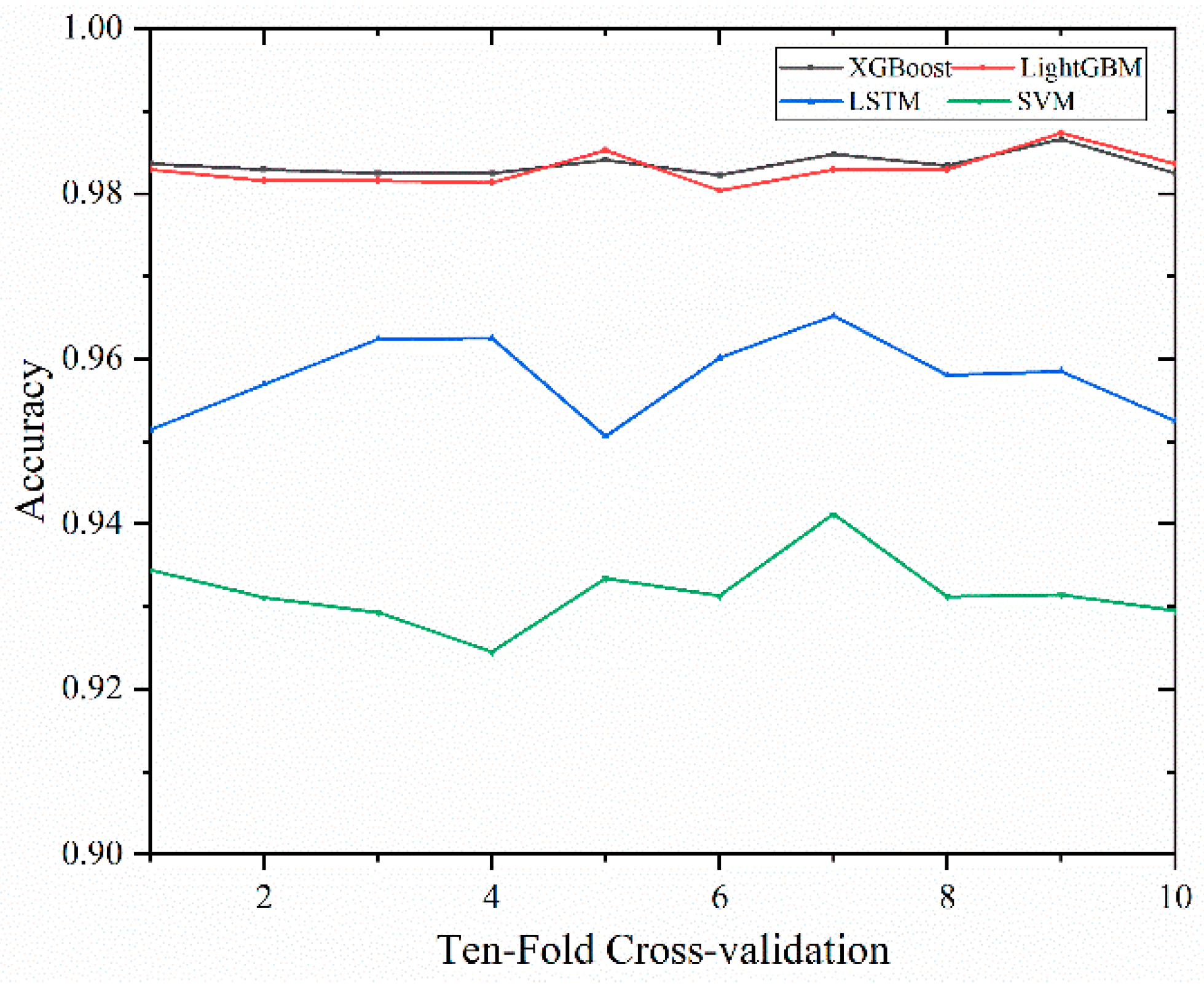
  • The results of this study indicate that, with an input length of 150 frames, the XGBoost and LightGBM models achieve an impressive overall classification performance of 98.4% and 98.3%, respectively. Compared to the LSTM and SVM models, the results show that the two ensemble models reduce the impact of Types I and III errors, improving accuracy by approximately 3.0%. With approximately equal classification performance, it is noteworthy that the XGBoost model required six times more training time than the LightGBM model.
  • The findings of this study should be helpful in the development of accurate and efficient models for LC recognition intentions in automated vehicles. Vehicle trajectories are accumulations of a series of driving behaviors. This study developed a real-time detection model for LC intention using vehicle trajectory data. Such models would aid road safety by facilitating intelligent interactions in automated driving and holding crucial implications for future traffic systems and urban planning.
  • This study has some limitations. First, only four existing models were compared. However, a broader array of models should be included in the comparison. Second, new models with superior performance may be developed in the future by amalgamating the strengths of existing models. Third, this study retained samples with only one lane-change, and samples with two or more lane-changes were all removed. Future studies should consider continuous lane-changing behavior. Finally, this study exclusively used the CitySim dataset, and future research should contemplate using a more extensive range of datasets to validate the findings of this study further.

Author Contributions

Conceptualization, R.Y. and C.W.; methodology, software, R.Y.; validation, R.Y. and S.D.; writing—original draft preparation, R.Y.; writing—review and editing, S.D. All authors have read and agreed to the published version of the manuscript.

Funding

This research received no external funding.

Data Availability Statement

Data is unavailable due to privacy or ethical restrictions. However, raw data can be requested through this website (https://github.com/ozheng1993/UCF-SST-CitySim-Dataset (Accessed on 20 June 2023)).

Conflicts of Interest

The authors declare no conflict of interest.

References

  1. Xu, T.; Zhang, Z.; Wu, X.; Qi, L.; Han, Y. Recognition of lane-changing behaviour with machine learning methods at freeway off-ramps. Phys. A Stat. Mech. Its Appl. 2021, 567, 125691. [Google Scholar] [CrossRef]
  2. Zhang, Y.; Chen, Y.; Gu, X.; Sze, N.; Huang, J. A proactive crash risk prediction framework for lane-changing behavior incorporating individual driving styles. Accid. Anal. Prev. 2023, 188, 107072. [Google Scholar] [CrossRef]
  3. Yuan, R.; Abdel-Aty, M.; Gu, X.; Zheng, O.; Xiang, Q. A Unified Approach to Lane Change Intention Recognition and Driving Status Prediction through TCN-LSTM and Multi-Task Learning Models. arXiv 2023, arXiv:2304.13732. [Google Scholar]
  4. Yuan, R.; Abdel-Aty, M.; Xiang, Q.; Wang, Z.; Zheng, O. A Novel Temporal Multi-Gate Mixture-of-Experts Approach for Vehicle Trajectory and Driving Intention Prediction. arXiv 2023, arXiv:2308.00533. [Google Scholar]
  5. Zhao, Y.; Zhou, J.; Zhao, C.; Li, M. Traffic Risk Assessment of Lane-Changing Process in Urban Inter-Tunnel Weaving Segment. Transp. Res. Rec. 2023, 2677, 03611981231160171. [Google Scholar] [CrossRef]
  6. Zhao, Y.; Wang, Z.; Wu, Y.; Ma, J. Trajectory-based characteristic analysis and decision modeling of the lane-changing process in intertunnel weaving sections. PLoS ONE 2022, 17, e0266489. [Google Scholar] [CrossRef] [PubMed]
  7. Zheng, B.; Hong, Z.; Tang, J.; Han, M.; Chen, J.; Huang, X. A Comprehensive Method to Evaluate Ride Comfort of Autonomous Vehicles under Typical Braking Scenarios: Testing, Simulation and Analysis. Mathematics 2023, 11, 474. [Google Scholar] [CrossRef]
  8. Xu, G.; Liu, L.; Song, Z. Driver behavior analysis based on Bayesian network and multiple classifiers. In Proceedings of the 2010 IEEE International Conference on Intelligent Computing and Intelligent Systems, Xiamen, China, 29–31 October 2010. [Google Scholar]
  9. Kumar, P.; Perrollaz, M.; Lefevre, S.; Laugier, C. Learning-Based Approach for Online Lane Change Intention Prediction. In Proceedings of the 2013 IEEE Intelligent Vehicles Symposium (IV), Gold Coast, Australia, 23–26 June 2013; pp. 797–802. (In English). [Google Scholar]
  10. Moridpour, S.; Sarvi, M.; Rose, G. Lane changing models: A critical review. Transp. Lett. 2010, 2, 157–173. [Google Scholar] [CrossRef]
  11. Deng, Q.; Wang, J.; Hillebrand, K.; Benjamin, C.R.; Söffker, D. Prediction performance of lane changing behaviors: A study of combining environmental and eye-tracking data in a driving simulator. IEEE Trans. Intell. Transp. Syst. 2019, 21, 3561–3570. [Google Scholar] [CrossRef]
  12. Doshi, A.; Trivedi, M. A Comparative Exploration of Eye Gaze and Head Motion Cues for Lane Change Intent Prediction. In Proceedings of the 2008 IEEE Intelligent Vehicles Symposium, Eindhoven, Netherlands, 4–6 June 2008; Volumes 1–3; pp. 1180–1185. (In English). [Google Scholar]
  13. Xing, Y.; Lv, C.; Wang, H.; Cao, D.; Velenis, E. An ensemble deep learning approach for driver lane-change intention inference. Transp. Res. Part C Emerg. Technol. 2020, 115, 102615. [Google Scholar] [CrossRef]
  14. Wang, L.; Yang, M.; Li, Y.; Hou, Y. A model of lane-changing intention induced by deceleration frequency in an automatic driving environment. Phys. A Stat. Mech. Its Appl. 2022, 604, 127905. [Google Scholar] [CrossRef]
  15. Morris, B.; Doshi, A.; Trivedi, M. Lane change intent prediction for driver assistance: On-road design and evaluation. In Proceedings of the 2011 IEEE Intelligent Vehicles Symposium (IV), Baden-Baden, Germany, 5–9 June 2011; IEEE: Piscataway, NJ, USA, 2011; pp. 895–901. [Google Scholar]
  16. Xing, Y.; Lv, C.; Wang, H.; Wang, H.; Ai, Y.; Cao, D.; Velenis, E.; Wang, F.Y. Driver lane-change intention inference for intelligent vehicles: Framework, survey, and challenges. IEEE Trans. Veh. Technol. 2019, 68, 4377–4390. [Google Scholar] [CrossRef]
  17. Li, K.; Wang, X.; Xu, Y.; Wang, J. Lane changing intention recognition based on speech recognition models. Transp. Res. Part C Emerg. Technol. 2016, 69, 497–514. [Google Scholar] [CrossRef]
  18. Dang, R.; Zhang, F.; Wang, J.; Yi, S.; Li, K. Analysis of Chinese driver’s lane change characteristic based on real vehicle tests in highway. In Proceedings of the 16th International IEEE Conference on Intelligent Transportation Systems (ITSC 2013), The Hague, the Netherlands, 6–9 October 2013; IEEE: Piscataway, NJ, USA, 2013; pp. 1917–1922. [Google Scholar]
  19. Zheng, J.; Suzuki, K.; Fujita, M. Predicting driver’s lane-changing decisions using a neural network model. Simul. Model. Pract. Theory 2014, 42, 73–83. [Google Scholar] [CrossRef]
  20. Ng, C.; Susilawati, S.; Kamal, M.A.S.; Chew, I.M.L. Development of a binary logistic lane change model and its validation using empirical freeway data. Transp. B Transp. Dyn. 2020, 8, 49–71. [Google Scholar] [CrossRef]
  21. Shi, Q.; Zhang, H. An improved learning-based LSTM approach for lane change intention prediction subject to imbalanced data. Transp. Res. Part C Emerg. Technol. 2021, 133, 103414. [Google Scholar] [CrossRef]
  22. Park, M.; Jang, K.; Lee, J.; Yeo, H. Logistic regression model for discretionary lane changing under congested traffic. Transp. A Transp. Sci. 2015, 11, 333–344. [Google Scholar] [CrossRef]
  23. McCall, J.C.; Wipf, D.P.; Trivedi, M.M.; Rao, B.D. Lane Change Intent Analysis Using Robust Operators and Sparse Bayesian Learning. IEEE Trans. Intell. Transp. Syst. 2007, 8, 431–440. [Google Scholar] [CrossRef]
  24. Izquierdo, R.; Parra, I.; Munoz-Bulnes, J.; Fernandez-Llorca, D.; Sotelo, M.A. Vehicle trajectory and lane change prediction using ANN and SVM classifiers. In Proceedings of the 2017 IEEE 20th International Conference on Intelligent Transportation Systems (ITSC), Yokohama, Japan, 16–19 October 2017. [Google Scholar]
  25. Gao, J.; Murphey, Y.L.; Yi, J.; Zhu, H. A data-driven lane-changing behavior detection system based on sequence learning. Transp. B Transp. Dyn. 2020, 10, 831–848. [Google Scholar] [CrossRef]
  26. Ali, Y.; Hussain, F.; Bliemer, M.C.J.; Zheng, Z.; Haque, M.M. Predicting and explaining lane-changing behaviour using machine learning: A comparative study. Transp. Res. Part C Emerg. Technol. 2022, 145, 103931. [Google Scholar] [CrossRef]
  27. Ding, S.; Abdel-Aty, M.; Zheng, O.; Wang, Z.; Wang, D. Traffic flow clustering framework using drone video trajectories to identify surrogate safety measures. arXiv 2023, arXiv:2303.16651. [Google Scholar] [CrossRef]
  28. Zheng, O. Development, Validation, and Integration of AI-Driven Computer Vision System and Digital-Twin System for Traffic Safety Dignostics. Ph.D. Thesis, University of Central Florida, Orlando, FL, USA, 2023. [Google Scholar]
  29. Zheng, O.; Abdel-Aty, M.; Yue, L.; Abdelraouf, A.; Wang, Z.; Mahmoud, N. CitySim: A Drone-Based Vehicle Trajectory Dataset for Safety Oriented Research and Digital Twins. arXiv 2022, arXiv:2208.11036. [Google Scholar] [CrossRef]
  30. Gu, X.; Abdel-Aty, M.; Xiang, Q.; Cai, Q.; Yuan, J. Utilizing UAV video data for in-depth analysis of drivers’ crash risk at interchange merging areas. Accid. Anal. Prev. 2019, 123, 159–169. [Google Scholar] [CrossRef] [PubMed]
  31. Coifman, B.; Li, L. A critical evaluation of the Next Generation Simulation (NGSIM) vehicle trajectory dataset. Transp. Res. Part B Methodol. 2017, 105, 362–377. [Google Scholar] [CrossRef]
  32. Chen, T.; Guestrin, C. XGBoost. In Proceedings of the 22nd ACM SIGKDD International Conference on Knowledge Discovery and Data Mining, San Francisco, CA, USA, 13–17 August 2016. [Google Scholar]
  33. Ke, G.; Meng, Q.; Finley, T.; Wang, T.; Chen, W.; Ma, W.; Ye, Q.; Liu, T.Y. LightGBM: A highly efficient gradient boosting decision tree. In Proceedings of the 31st International Conference on Neural Information Processing Systems, Long Beach, CA, USA, 4–9 December 2017. [Google Scholar]
  34. Yang, D.; Wu, Y.; Sun, F.; Chen, J.; Zhai, D.; Fu, C. Freeway accident detection and classification based on the multi-vehicle trajectory data and deep learning model. Transp. Res. Part C Emerg. Technol. 2021, 130, 103303. [Google Scholar] [CrossRef]
  35. Bocklisch, F.; Bocklisch, S.F.; Beggiato, M.; Krems, J.F. Adaptive fuzzy pattern classification for the online detection of driver lane change intention. Neurocomputing 2017, 262, 148–158. [Google Scholar] [CrossRef]
  36. Schiro, J.; Loslever, P.; Gabrielli, F.; Pudlo, P. Inter and intra-individual differences in steering wheel hand positions during a simulated driving task. Ergonomics 2015, 58, 394–410. [Google Scholar] [CrossRef]
Figure 1. A snapshot of the freeway-B segment.
Infrastructures 08 00156 g001
Figure 2. Comparison of original trajectory and processed trajectory.
Infrastructures 08 00156 g002
Figure 3. The subject vehicle and surrounding vehicles.
Infrastructures 08 00156 g003
Figure 4. The impact of the decision tree number on recognition accuracy and training time.
Infrastructures 08 00156 g004
Figure 5. Accuracy comparison of LSTM, SVM, XGBoost, and LightGBM.
Infrastructures 08 00156 g005
Figure 6. Ten-fold cross-validation for LSTM, SVM, XGBoost, and LightGBM.
Infrastructures 08 00156 g006
Figure 7. Confusion matrix of classification models.
Infrastructures 08 00156 g007
Table 1. Input variables.
NotationVariableDescription
vx-iLongitudinal velocityLongitudinal velocities of the target and surrounding vehicles are separately considered. (ft/sec)
vy-iLateral velocityLateral velocities of the target and surrounding vehicles are separately considered. (ft/sec)
ax-iLongitudinal accelerationLongitudinal accelerations of the target and surrounding vehicles are separately considered. (ft/sec2)
ay-iLateral accelerationLateral accelerations of the target and surrounding vehicles are separately considered. (ft/sec2)
θ-iVehicle headingVehicle headings of the target and surrounding vehicles are separately considered.
Δθ-iYawRateYaw rates of the target and surrounding vehicles are separately considered.
dw-uHeadwayThe distance between the target vehicle and surrounding vehicles.
Val-uState variable0 means it has recorded trajectory information; 1 means the trajectory information is missing.
Table 2. Evaluation results of LSTM, SVM, XGBoost, and LightGBM.
ModelTypePrecisionRecallAccuracyTraining Time (s)
LSTMLK90.10%96.21%95.33%992.3
RLC97.83%95.78%
LLC97.79%93.73%
SVMLK88.31%97.29%94.21%33,819.3
RLC97.23%93.46%
LLC96.88%92.10%
XGBoostLK95.29%99.88%98.42%3850.7
RLC99.93%97.92%
LLC99.96%97.50%
LightGBMLK99.91%94.98%98.32%496.4
RLC97.89%99.93%
LLC97.34%100%
Disclaimer/Publisher’s Note: The statements, opinions and data contained in all publications are solely those of the individual author(s) and contributor(s) and not of MDPI and/or the editor(s). MDPI and/or the editor(s) disclaim responsibility for any injury to people or property resulting from any ideas, methods, instructions or products referred to in the content.

