
Framework for Smart Cost Optimization of Material Logistics in Construction Road Projects


Abstract
:1. Introduction
2. Literature Review
2.1. IoT Studies
2.2. Supplier Selection Criteria Studies
|
|
|
|
|
|
|
|
|
|
|
|
|
|
|
|
|
|
|
|
|
|
|
|
2.3. Supplier Selection Methods
- Statistical/probabilistic (cluster analysis), such as fuzzy set theory.
- Multi-attribute decision making (categorial methods), such as AHP, ANP, TOPSIS, MAUT, and outranking methods such as ELECTRE and PROMOTHEE.
- Methods based on costs, such as ABC and TCO.
- Mathematical programming (data envelopment analysis), such as LP, MOLP, and goal programming.
- AI, such as CBR and ANN.
- Combined approaches, such as (MP + TCO, AHP + LP, MAUT + LP, ANP + TOPSIS, and fuzzy TOPSIS).
2.4. Studies Related to LP Methods of Optimizing Material Supply Chain
2.5. Studies Related to Location Data Accuracy for Optimizing Material Supply Chain
2.6 Studies Related to Data Validation for Optimizing Material Supply Chain Using BC
2.7. Studies Related to CSM in Optimizing Material Supply Chain
2.8. Studies Related to ICT Technology CSM in Optimizing Material Supply Chain
2.9. Smart Networks and IoT-Based Real-Time Production Logistics
2.10. Discussion of the Gap of Knowledge in This Study
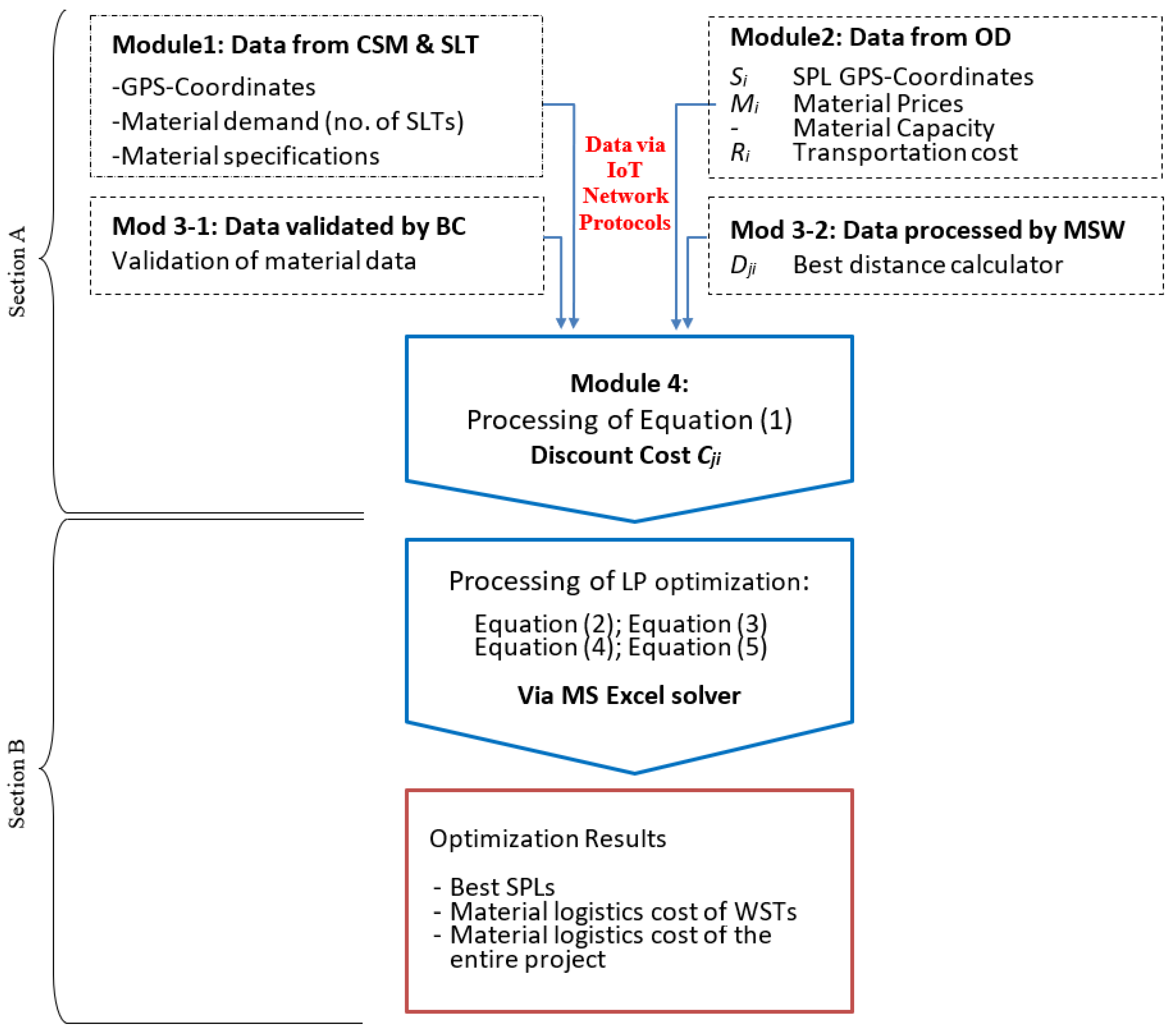
3. Flowchart of the Proposed Smart Framework for Logistics Cost Optimization
3.1. Section A: Collecting and Validating of Dynamic Input Data of Material Logistics Cost
- Material demand volume (denoted by variable Tj) is required for the current WST. The active CSM working at the current position predicts this material demand volume. The variable counts the number of fully-loaded SLTs needed to cover the demand of this site.
- GPS coordinates of the current WST (latitude and longitude). These data are fed permanently by the active CSM and used by the MSW to determine the distance between the current WST and potential SPLs.
- Type of construction materials required to the current WST.
- GPS coordinates of trusted SPL (exact latitude and longitude);
- Material transportation price per km (Ri);
- Material types available by SPLs (M-types, such as M1, M2, and M3);
- Capacity: the maximum count of fully loaded SLTs that SPL can send (the quantity unit of the transported material is measured by the count of fully loaded SLTs, not m3);
- The material price, which is updated dynamically by SPLs (Mi).
- T: Material demand (number of fully loaded SLTs needed for current WST);
- D: Accurate logistics distance (derived from MSW);
- R: Updated transportation cost per km (imported from OD and proved by BC);
- V: Constant SLT volume equals 30 m3 (max. 24 ton);
- M: Material procurement cost per m3 (imported from OD and proved by BC).
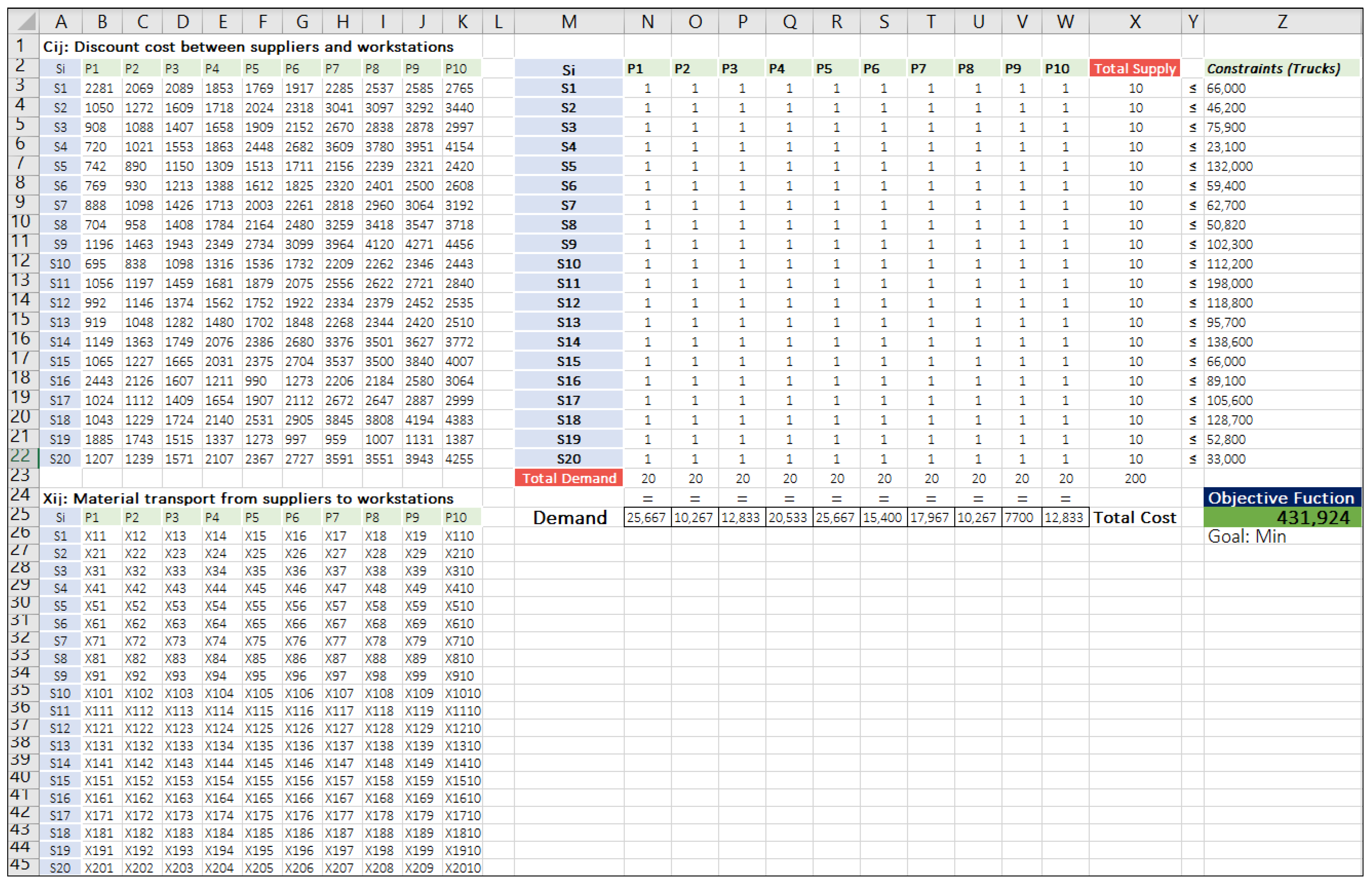
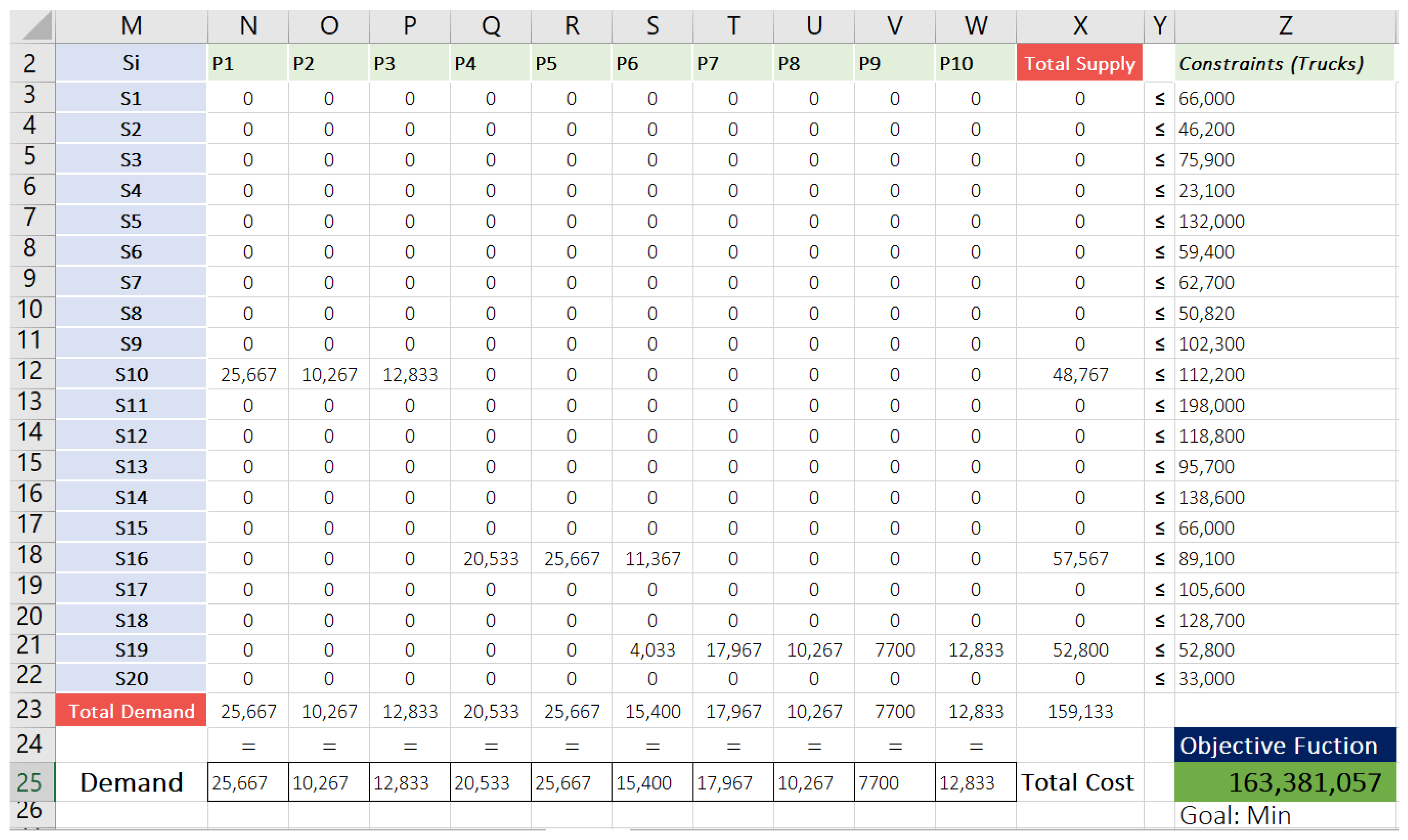
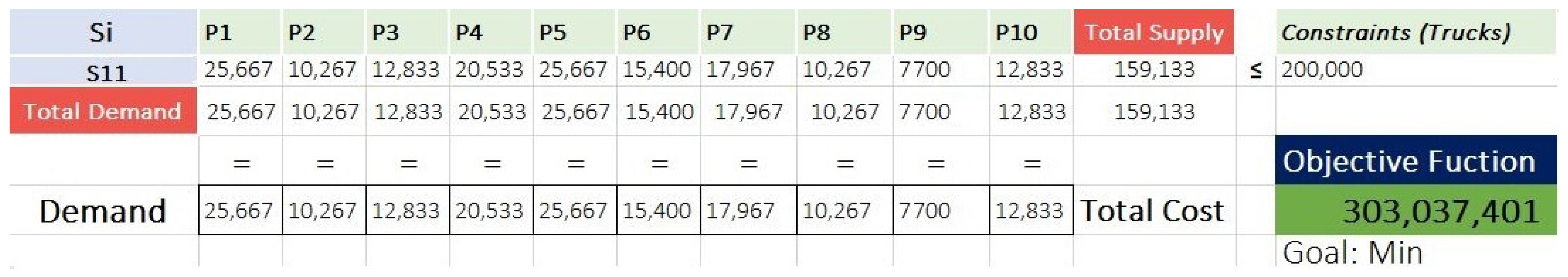
3.2. Section B: Applying LP Optimization Functions by MS Excel Solver
- Conceptualize sourcing of raw material for road construction as a logistics optimization problem.
- Formulate the LP model for the given problem statement and implied resource constraints.
- Solve the LP formulation by an optimization solver.
- Interpret the final output of the solver to determine the quantity to be procured from each supplier and distributed through various demand locations of the road.
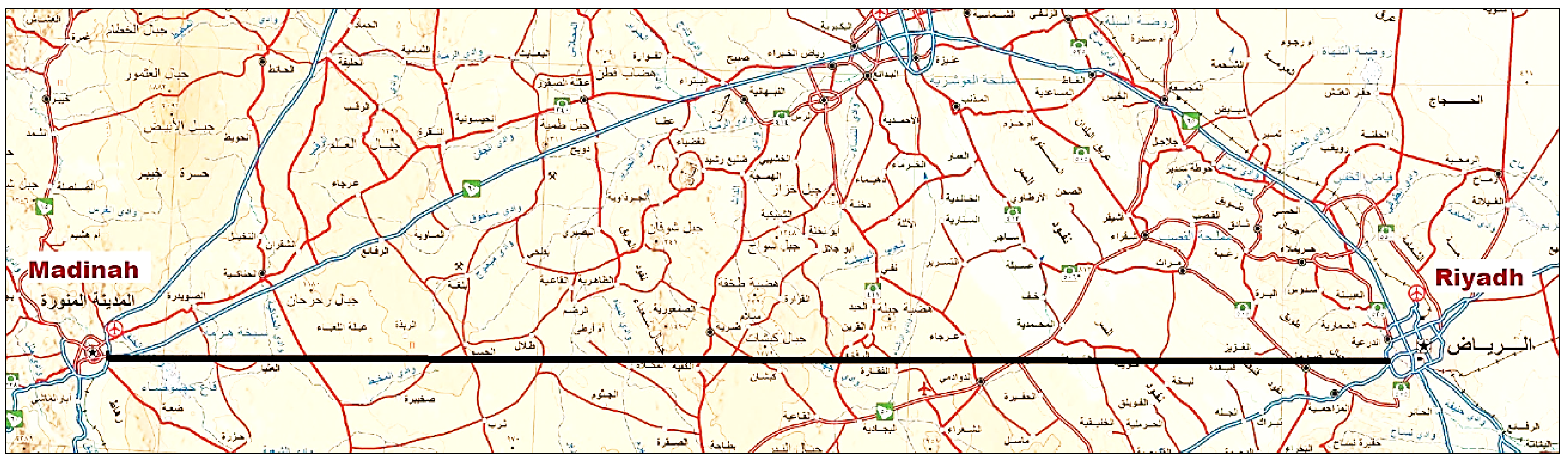
4. Case Study: Enhancing Material Logistics Cost with a Smart Framework
4.1. Case Study Description
4.2. Applying Case Study with the Proposed Framework
4.3. Results and Discussion of the Case Study
- j = 3, which refers to WST P3
- I = 2, which refers to SPL S2
- T3 = 1, which represents one full loaded SLT of limestone collected from WST P3
- D3,2 = 242 km, where this value is derived from MSW (Module 3), which imports
- R2 = SAR 3.30 for one fully loaded SLT per km. These data were imported from Module (2) and validated by Module (3).
- VT = 30 m3 SLT volume (max. 24 ton). This value is constant.
- M2 = SAR 27 per m3. Module (2) and (3) imported and validated these data.
4.4. Validation of the Smart Framework
= 700,000 m × 22 m × 0.50 m × 4.78 SAR/m3
= SAR 36,806,000
4.5. Sensitivity Analysis
5. Conclusions
Author Contributions
Funding
Institutional Review Board Statement
Informed Consent Statement
Data Availability Statement
Acknowledgments
Conflicts of Interest
Abbreviations
| IoT | internet of things |
| DC | data connectivity |
| BC | blockchain |
| AI | artificial intelligence |
| KSA | Kingdom of Saudi Arabia |
| LP | linear programming |
| GPS | global positioning system |
| MIM | ministry of industry and mineral resources |
| OD | governmental open data |
| MSW | mapping software |
| CSM | construction smart machine |
| WST | workstation |
| SPL | supplier |
| SAR | Saudi Arabian Riyal (currency) |
| MM | million |
| j | index of workstations |
| i | index of suppliers |
| Pj | symbol of workstation |
| Si | symbol of supplier |
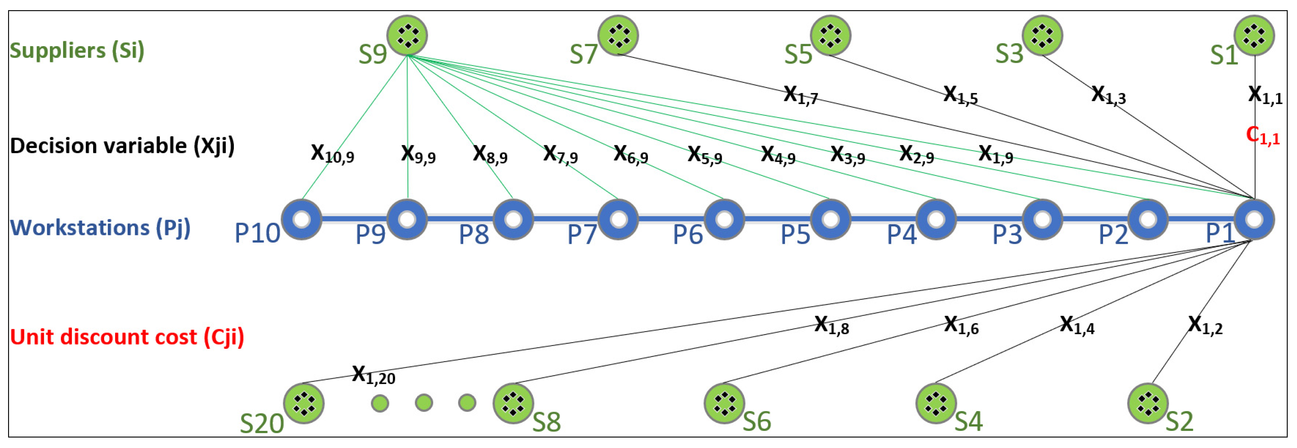
| Xji | decision variable of unit quantity for shipping material from SPL to WST |
| Cji | variable of unit discount cost for shipped material. |
| Dji | distance variable measured by MSW to ship material from SPL to WST. |
| Tj | unit demand of material (loaded SLT) needed for WST j |
| Ri | transportation price per km and SLT |
| Mi | dynamically updated material prices offered by SPL. |
| V | SLT volume |
| ρi | maximum supply capacity of raw material available by SPL |
| μj | total demand of raw material (loaded SLTs) needed for WST j |
| km | kilometer |
References
- SPA, Saudi Press Agency. Available online: https://www.spa.gov.sa/viewfullstory.php?lang=en&newsid=2109234 (accessed on 20 December 2021).
- BCS. The Chartered Institute for IT. Available online: https://www.bcs.org/articles-opinion-and-research/10-disruptive-technologies-and-how-they-ll-change-your-life/ (accessed on 20 December 2021).
- Saudi Gazette. Available online: https://saudigazette.com.sa/article/590331 (accessed on 20 December 2021).
- CITC, Communications and Information Technology Commission. Available online: https://www.citc.gov.sa/en/researchs-studies/research-innovation/Documents/CITC-IoT_Demand.pdf (accessed on 20 December 2021).
- Gul, R. Impact of Rural Road Construction in Local Economy in Afghanistan. Master’s Thesis, Kardan University, Kabul, Afghanistan, 2020. [Google Scholar]
- Choudhari, S.; Tindwani, A. Logistics optimisation in road construction project. Constr. Innov. 2017, 17, 158–179. [Google Scholar] [CrossRef]
- Jaziri, R.; Korbi, K.; Gontara, S. The Application of Physical Internet in Saudi Arabia—Towards a Logistic Hub in 2030. J. Manag. Train. Ind. 2020, 7, 1–16. [Google Scholar] [CrossRef]
- Issaoui, Y.; Khiat, A.; Bahnasse, A.; Hassan, O. Smart Logistics: Blockchain trends and applications. J. Ubiquitous Syst. Pervasive Netw. 2020, 12, 9–15. [Google Scholar] [CrossRef]
- Karakostas, B. A DNS Architecture for the Internet of Things: A Case Study in Transport Logistics. Procedia Comput. Sci. 2013, 19, 594–601. [Google Scholar] [CrossRef] [Green Version]
- Kumar, N.; Dash, A. The Internet of Things: An Opportunity for Transportation and Logistics. In Proceedings of the International Conference on Inventive Computing and Informatics, Coimbatore, India, 1 November 2017. [Google Scholar]
- Witkowski, K. Internet of Things, Big Data, Industry 4.0—Innovative Solutions in Logistics and Supply Chains Management. Procedia Eng. 2017, 182, 763–769. [Google Scholar] [CrossRef]
- Nabto. Available online: https://www.nabto.com/guide-iot-protocols-standards/ (accessed on 27 March 2022).
- Cengiz, A.E.; Aytekin, O.; Ozdemir, I.; Kusan, H.; Çabuk, A. A Multi-criteria Decision Model for Construction Material Supplier Selection. Procedia Eng. 2017, 196, 294–301. [Google Scholar] [CrossRef]
- Taherdoost, H.; Brard, A. Analysing the Process of Supplier Selection Criteria and Methods. Procedia Manuf. 2019, 32, 1024–1034. [Google Scholar] [CrossRef]
- Singh, R.K.; Modgil, S. Supplier selection using SWARA and WASPAS—A case study of Indian cement industry. Meas. Bus. Excel. 2020, 24, 243–265. [Google Scholar] [CrossRef]
- Mukherjee, K. Supplier selection criteria and methods: Past, present and future. Int. J. Oper. Res. 2016, 27, 356–373. [Google Scholar] [CrossRef]
- Tahriri, F.; Osman, M.; Ali, A.; Yusuff, R. A review of supplier selection methods in manufacturing industries. Suranaree J. Sci. Technol. 2008, 15, 201–208. [Google Scholar]
- Ali, I.; Fügenschuh, A.; Gupta, S.; Modibbo, U.M. The LR-Type Fuzzy Multi-Objective Vendor Selection Problem in Supply Chain Management. Mathematics 2020, 8, 1621. [Google Scholar] [CrossRef]
- Nazari-Shirkouhi, S.; Shakouri, H.; Javadi, B.; Keramati, A. Supplier selection and order allocation problem using a two-phase fuzzy multi-objective linear programming. Appl. Math. Model. 2013, 37, 9308–9323. [Google Scholar] [CrossRef]
- Liao, C.-N.; Kao, H.-P. An integrated fuzzy TOPSIS and MCGP approach to supplier selection in supply chain management. Expert Syst. Appl. 2011, 38, 10803–10811. [Google Scholar] [CrossRef]
- Jadidi, O.; Zolfaghari, S.; Cavalieri, S. A new normalized goal programming model for multi-objective problems: A case of supplier selection and order allocation. Int. J. Prod. Econ. 2014, 148, 158–165. [Google Scholar] [CrossRef]
- Uygun, O.; Kaçamak, H.; Kahraman, Ü.A. An integrated DEMATEL and Fuzzy ANP techniques for evaluation and selection of outsourcing provider for a telecommunication company. Comput. Ind. Eng. 2015, 86, 137–146. [Google Scholar] [CrossRef]
- Astanti, R.D.; Mbolla, S.E.; Ai, T.J. Raw material supplier selection in a glove manufacturing: Application of AHP and fuzzy AHP. Decis. Sci. Lett. 2020, 9, 291–312. [Google Scholar] [CrossRef]
- Sobotka, A.; Jaskowski, P.; Czarnigowsk, A. Optimisation of Aggregate Supplies for Road Projects. Procedia-Soc. Behav. Sci. 2012, 48, 838–846. [Google Scholar] [CrossRef] [Green Version]
- Xiaojiang, Y. Optimization Algorithm of Logistics Transportation Cost of Prefabricated Building Components for Project Management. J. Math. 2022, 2022, 9. [Google Scholar]
- De Lima, R.; Júnior, E.; Prata, B.; Weissmann, J. Distribution of materials in road earthmoving and paving: Mathematical programming approach. J. Constr. Eng. Manag. 2013, 139, 1046–1054. [Google Scholar] [CrossRef] [Green Version]
- Arayapan, K.; Warunyuwong, P. Logistics optimisation: Application of Optimisation Modeling in Inbound Logistics. Master’s Thesis, Mälardalen University, Västerås, Sweden, 2009. [Google Scholar]
- Fathi, M.; Bevrani, H. Optimisation in Electrical Engineering; Springer: Cham, Switzerland, 2019. [Google Scholar]
- Sammut, C.; Webb, G. Data Preparation. In Encyclopedia of Machine Learning and Data Mining; Springer: Boston, MA, USA, 2017. [Google Scholar]
- Beskorovainyi, V.; Kuropatenko, O.; Gobov, D. Optimisation of transportation routes in a closed logistics system. Innov. Technol. Sci. Solut. Ind. 2019, 4, 24–32. [Google Scholar]
- Zhao, X.; Carling, K.; Håkansson, J. An Evaluation of the Reliability of GPS-Based Transportation Data. In Proceedings of the Computer Science Conference, Vienna, Austria, 24 November 2017. [Google Scholar]
- Cedillo-Campos, M.; Pérez-González, C.; Piña-Barcena, J.; Moreno-Quintero, E. Measurement of travel time reliability of road transportation using GPS data: A freight fluidity approach. Transp. Res. Part A Policy Pract. 2019, 130, 240–288. [Google Scholar] [CrossRef]
- Devlin, G.; McDonnell, K.; Ward, S. Performance Accuracy of Low-Cost Dynamic Non-Differential GPS On Articulated Trucks. Appl. Eng. Agric. Am. Soc. Agric. Biol. Eng. 2007, 23, 273–279. [Google Scholar]
- Somplak, R.; Smidova, Z.; Smejkalova, V.; Nevrly, V. Statistical Evaluation of Large-Scale Data Logistics System. Mendel 2018, 24, 9–16. [Google Scholar] [CrossRef]
- Farouk, M.; Darwish, S. Reverse Logistics Solution in e-Supply Chain Management by Blockchain Technology. Egypt. Comput. Sci. J. 2020, 44, 1110–2586. [Google Scholar]
- Penzes, B. Blockchain Technology in the Construction Industry; Institute of Civil Engineers: London, UK, 2018. [Google Scholar]
- Ganne, E. Can Blockchain Revolutionise International Trade? World Trade Organization: Geneva, Switzerland, 2018; ISBN 978-92-870-4761-8. [Google Scholar]
- Japan Gov. Available online: https://www.japan.go.jp/tomodachi/2017/autumn2017/power_of_innovation.html (accessed on 23 January 2022).
- Evans, V.; Horak, J. Sustainable Urban Governance Networks, Data-driven Internet of Things Systems, and Wireless Sensor-based Applications in Smart City Logistics. JSTOR Geopolit. Hist. Int. Relat. 2021, 13, 65–78. [Google Scholar]
- Nica, E.; Stan, C.I.; Luțan, A.G.; Oașa, R.-Ș. Internet of Things-based Real-Time Production Logistics, Sustainable Industrial Value Creation, and Artificial Intelligence-driven Big Data Analytics in Cyber-Physical Smart Manufacturing Systems. Econ. Manag. Financ. Mark. 2021, 16, 52–62. [Google Scholar]
- Popescu, G.H.; Petreanu, S.; Alexandru, B.; Corpodean, H. Internet of Things-based Real-Time Production Logistics, Cyber-Physical Process Monitoring Systems, and Industrial Artificial Intelligence in Sustainable Smart Manufacturing. J. Self-Gov. Manag. Econ. 2021, 9, 52–62. [Google Scholar]
- Mays, W.; Tung, Y. Hydrosystems Engineering and Management. In Water-Supply Engineering; McGraw-Hill: New York, NY, USA, 1992; pp. 54–90. [Google Scholar]
- GASGI. General Authority for Survey and Geospatial Information. Available online: https://www.gasgi.gov.sa/en/pages/default.aspx (accessed on 3 February 2022).
- The Civil Engineering. Available online: https://thecivilengineerings.com/method-statement-for-asphalt-paving-works-asphalt-concrete/ (accessed on 29 January 2022).
- MIM. Ministry of Industry and Mineral Resources. Available online: https://dmmr.gov.sa/mop/Documents/MineralResourcesBook_Ar.pdf (accessed on 3 February 2022).


| Notation | Description |
|---|---|
| Index | |
| i | SPL index (from 1 to I) |
| j | WST index (from 1 to J) |
| Decision variables | |
| xij | Unit quantity of raw material shipped from Si to Pj |
| Parameters | |
| I | Total number of SPLs |
| J | Total number of WSTs |
| cij | Discount cost of transporting single unit of material from Si to Pj |
| ρi | The maximum supply capacity of raw material at source Si (per SLT) * |
| μj | The total demand of raw material at WST Pj (per SLT) * |
| Field Name | SPL S1 | SPL S2 | SPL S3 | … Si |
|---|---|---|---|---|
| location (city) | Jubail | Riyadh | Jeddah | … |
| GPS (lat., long.) | 27.15, 49.2 | 24.98, 46.99 | 21.47, 39.39 | … |
| raw material type | M1 | M3 | M1 | … |
| material description | limestone | silica sand | limestone | … |
| capacity (per SLT) | 210,372 | 135,621 | 77,235 | … |
| price (SAR/SLT) | SAR 830.00 | SAR 720.00 | SAR 980.00 | … |
| available transporters (SLTs) | 50 | 33 | 75 | … |
| transportation price (per SLT/km) | SAR 3.50 | SAR 4.00 | SAR 4.30 | … |
| quotation update time | 16/9/21 7:16 | 19/9/21 13:52 | 18/9/21 0:43 | … |
| WST Pj | Demand (SLTs) | SPL Si | Capacity (SLTs) | SPL Si | Capacity (SLTs) |
|---|---|---|---|---|---|
| P1 (depth = 0.5 m) | 25,667 | S1 | 66,000 | S11 | 198,000 |
| P2 (0.2 m) | 10,267 | S2 | 46,200 | S12 | 118,800 |
| P3 (0.25 m) | 12,833 | S3 | 75,900 | S13 | 95,700 |
| P4 (0.4 m) | 20,533 | S4 | 23,100 | S14 | 138,600 |
| P5 (0.5 m) | 25,667 | S5 | 132,000 | S15 | 66,000 |
| P6 (0.3 m) | 15,400 | S6 | 59,400 | S16 | 89,100 |
| P7 (0.35 m) | 17,967 | S7 | 62,700 | S17 | 105,600 |
| P8 (0.2 m) | 10,267 | S8 | 50,820 | S18 | 128,700 |
| P9 (0.15 m) | 7700 | S9 | 102,300 | S19 | 52,800 |
| P10 (0.25 m) | 12,833 | S10 | 112,200 | S20 | 33,000 |
| Si | P1 | P2 | P3 | P4 | P5 | P6 | P7 | P8 | P9 | P10 |
|---|---|---|---|---|---|---|---|---|---|---|
| S1 | 2281 | 2069 | 2089 | 1853 | 1769 | 1917 | 2285 | 2537 | 2585 | 2765 |
| S2 | 1050 | 1272 | 1609 | 1718 | 2024 | 2318 | 3041 | 3097 | 3292 | 3440 |
| S3 | 908 | 1088 | 1407 | 1658 | 1909 | 2152 | 2670 | 2838 | 2878 | 2997 |
| S4 | 720 | 1021 | 1553 | 1863 | 2448 | 2682 | 3609 | 3780 | 3951 | 4154 |
| S5 | 742 | 890 | 1150 | 1309 | 1513 | 1711 | 2156 | 2239 | 2321 | 2420 |
| S6 | 769 | 930 | 1213 | 1388 | 1612 | 1825 | 2320 | 2401 | 2500 | 2608 |
| S7 | 888 | 1098 | 1426 | 1713 | 2003 | 2261 | 2818 | 2960 | 3064 | 3192 |
| S8 | 704 | 958 | 1408 | 1784 | 2164 | 2480 | 3259 | 3418 | 3547 | 3718 |
| S9 | 1196 | 1463 | 1943 | 2349 | 2734 | 3099 | 3964 | 4120 | 4271 | 4456 |
| S10 | 695 | 838 | 1098 | 1316 | 1536 | 1732 | 2209 | 2262 | 2346 | 2443 |
| S11 | 1056 | 1197 | 1459 | 1681 | 1879 | 2075 | 2556 | 2622 | 2721 | 2840 |
| S12 | 992 | 1146 | 1374 | 1562 | 1752 | 1922 | 2334 | 2379 | 2452 | 2535 |
| S13 | 919 | 1048 | 1282 | 1480 | 1702 | 1848 | 2268 | 2344 | 2420 | 2510 |
| S14 | 1149 | 1363 | 1749 | 2076 | 2386 | 2680 | 3376 | 3501 | 3627 | 3772 |
| S15 | 1065 | 1227 | 1665 | 2031 | 2375 | 2704 | 3537 | 3500 | 3840 | 4007 |
| S16 | 2443 | 2126 | 1607 | 1211 | 990 | 1273 | 2206 | 2184 | 2580 | 3064 |
| S17 | 1024 | 1112 | 1409 | 1654 | 1907 | 2112 | 2672 | 2647 | 2887 | 2999 |
| S18 | 1043 | 1229 | 1724 | 2140 | 2531 | 2905 | 3845 | 3808 | 4194 | 4383 |
| S19 | 1885 | 1743 | 1515 | 1337 | 1273 | 997 | 959 | 1007 | 1131 | 1387 |
| S20 | 1207 | 1239 | 1571 | 2107 | 2367 | 2727 | 3591 | 3551 | 3943 | 4255 |
| Cost Type | SPL (A) | SPL (B) | SPL (C) | Optimal Unit Cost |
|---|---|---|---|---|
| SAR/m3 | SAR/m3 | SAR/m3 | SAR/m3 | |
| Average material price (excl. overhead cost) | 22.5 | 24 | 22 | 17.22 |
| Transported (+SAR 4.0) | 26.5 | 28 | 26 | 21.22 |
Publisher’s Note: MDPI stays neutral with regard to jurisdictional claims in published maps and institutional affiliations. |
© 2022 by the authors. Licensee MDPI, Basel, Switzerland. This article is an open access article distributed under the terms and conditions of the Creative Commons Attribution (CC BY) license (https://creativecommons.org/licenses/by/4.0/).
Share and Cite
Alanazi, A.; Al-Gahtani, K.; Alsugair, A. Framework for Smart Cost Optimization of Material Logistics in Construction Road Projects. Infrastructures 2022, 7, 62. https://doi.org/10.3390/infrastructures7050062
Alanazi A, Al-Gahtani K, Alsugair A. Framework for Smart Cost Optimization of Material Logistics in Construction Road Projects. Infrastructures. 2022; 7(5):62. https://doi.org/10.3390/infrastructures7050062
Chicago/Turabian StyleAlanazi, Abdulkareem, Khalid Al-Gahtani, and Abdullah Alsugair. 2022. "Framework for Smart Cost Optimization of Material Logistics in Construction Road Projects" Infrastructures 7, no. 5: 62. https://doi.org/10.3390/infrastructures7050062
APA StyleAlanazi, A., Al-Gahtani, K., & Alsugair, A. (2022). Framework for Smart Cost Optimization of Material Logistics in Construction Road Projects. Infrastructures, 7(5), 62. https://doi.org/10.3390/infrastructures7050062