
Bridge Inspection and Defect Recognition with Using Impact Echo Data, Probability, and Naive Bayes Classifiers


Abstract
:1. Introduction
- Developing a preprocessing approach based on distinguishable peak points;
- Using probabilistic methods to find a relative pattern for detecting defects or sound regions based on the features of the IE signals;
- Using probabilistic methods to find atypical IE data or data that does not follow the general pattern of IE signals in each dataset. Classification of the IE data in terms of defect or sound based on the feature of preprocessed IE signals.
2. Method
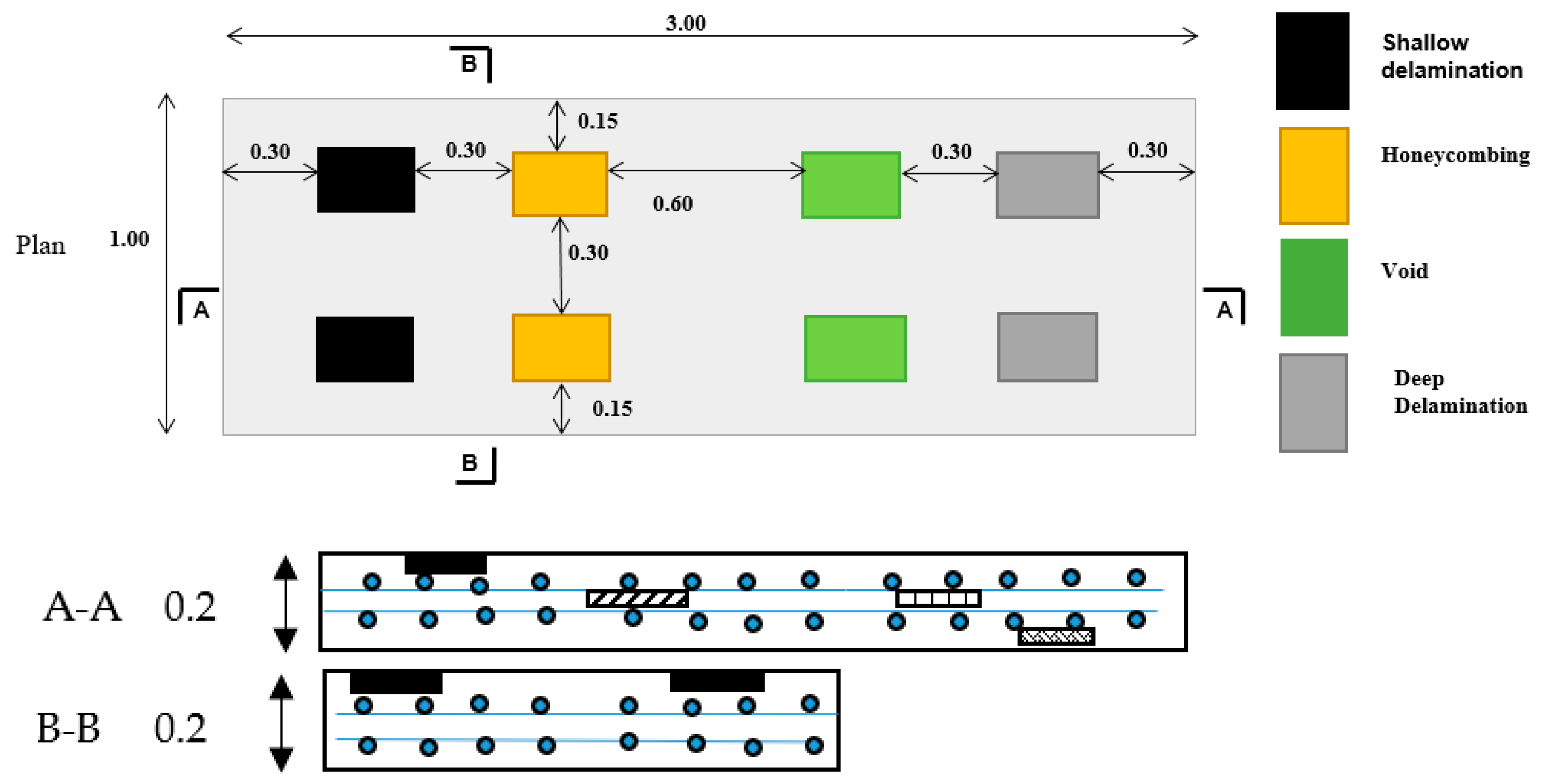
2.1. Description of Data
2.2. IE Method
2.3. Description of the Proposed Method
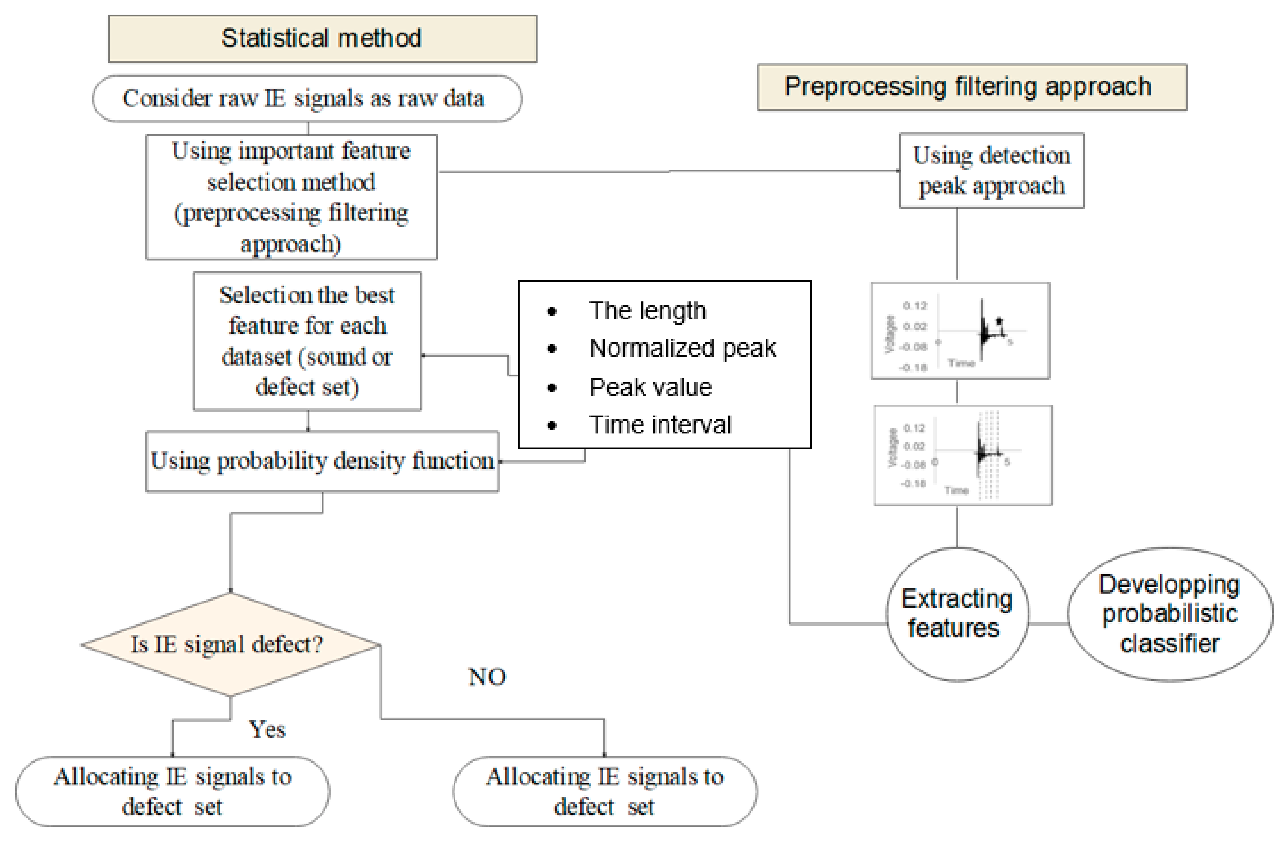
- The use of preprocessing filtering approach to detect distinguished peaks, which leads to statistical classification and detection of IE signals. The preprocessed IE signals were generated based on distinguished peaks in IE signals as seen Figure 3. Generally, the frequency domain corresponding to the peak point of IE signal has been employed to evaluate the behavior of IE signals in the frequency approach. However, some research in computer science shows the peak values of signals can be used to classify data in time domain [23]. To evaluate IE signals in time domain, detection peak algorithm was employed to cut signals based on distinguished points. To do this, as shown in Figure 3, any point with values less than 10% of the absolute maximum value was removed from the start and end of the IE signal. This will not have a major impact on the analysis, since peaks with values smaller than 10% of the absolute max will not change the frequency repose significantly. This claim was validated through applying the proposed preprocessing filtering approach on a set of random IE signals, which showed the frequency response of raw and processed signal impact echo signals were the same when the trivial points were removed. Finally, the IE signal was divided into five segments. Time domain (starts and end point), normalized peak values and length of preprocessed IE signals was obtained for each segment as the futures of IE signals.
- Probability and Naive Bayes classifiers were used to classify data. In the following, the statistical and Probabilistic classification was discussed.
- -
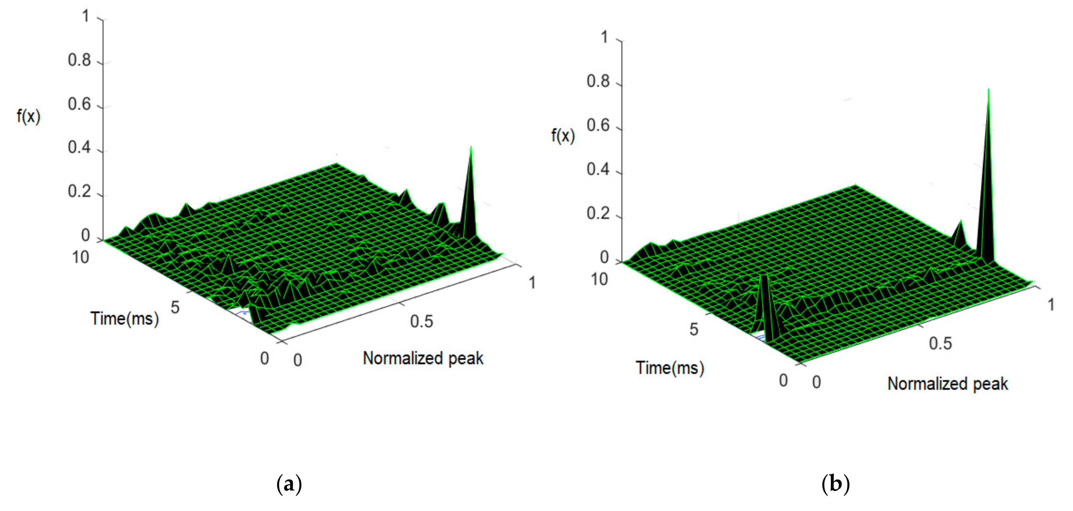
- Statistical methodThe probability density function (PDF) can be used to see the probability of occurrence of samples, it also can be used to remove outliers or atypical data from an original dataset. Understanding the PDF for a group of data could be useful to determine data distribution type, mean, and variance, special patterns for classifying. A set of PDFs for IE data were generated based on the feature of IE signals. Easy Fit [24] was used to fit a series of known probability distribution to the IE PDFs. Additionally, 3-D representation of pdf (probability density function (f(x))) were built to identify correlation between the variables.
- -
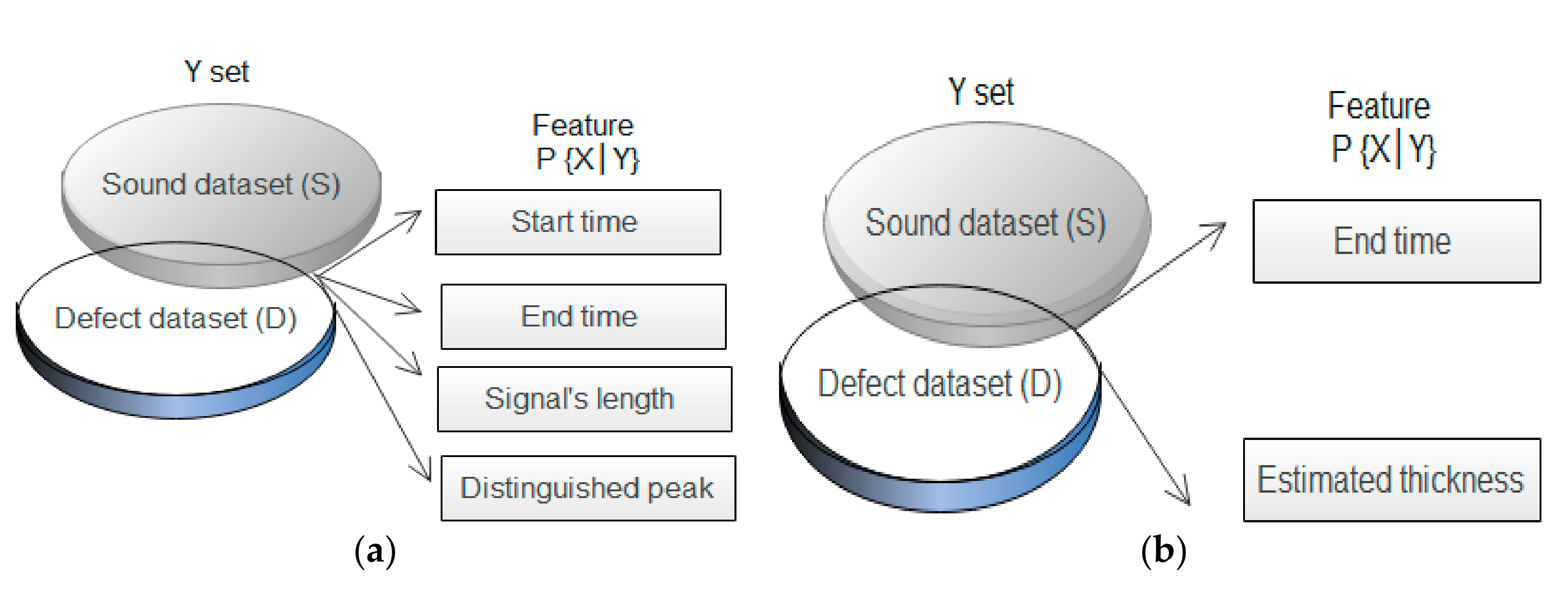
- Probabilistic classificationA probabilistic classifier is considered as a classification approach in machine learning, which is employed to estimate the probability that each data set occur with using input layers. Naive Bayes classifiers were employed for classification by applying Bayes’ theorem and independence assumptions between input layers [25]. In this research, the relationship between input variables such as signal peaks, length, end and start time of preprocessed signals, and the output layers (defect or sound area) was obtained. In addition, the relationship among the IE signal’s end time interval and the amount of the estimated thickness was evaluated. As seen in Figure 2, two models were generated as probabilistic classification models. For the first model, the input layer contained the length of signals, average of peak value, start and end time of preprocessed IE signals, and the output layers are defect and sound set. For the second, in the input layer is contained the estimated thickness, which was obtained using frequency approach and end time of preprocessed signals.
3. Results
- -
- First, the futures of IE signals in defected and sound regions were compared
- -
- The relationship between the estimated thickness, which was obtained by the frequency domain of IE signals, was compared to the features of signals in the time domain.
3.1. Statistical Result
- -
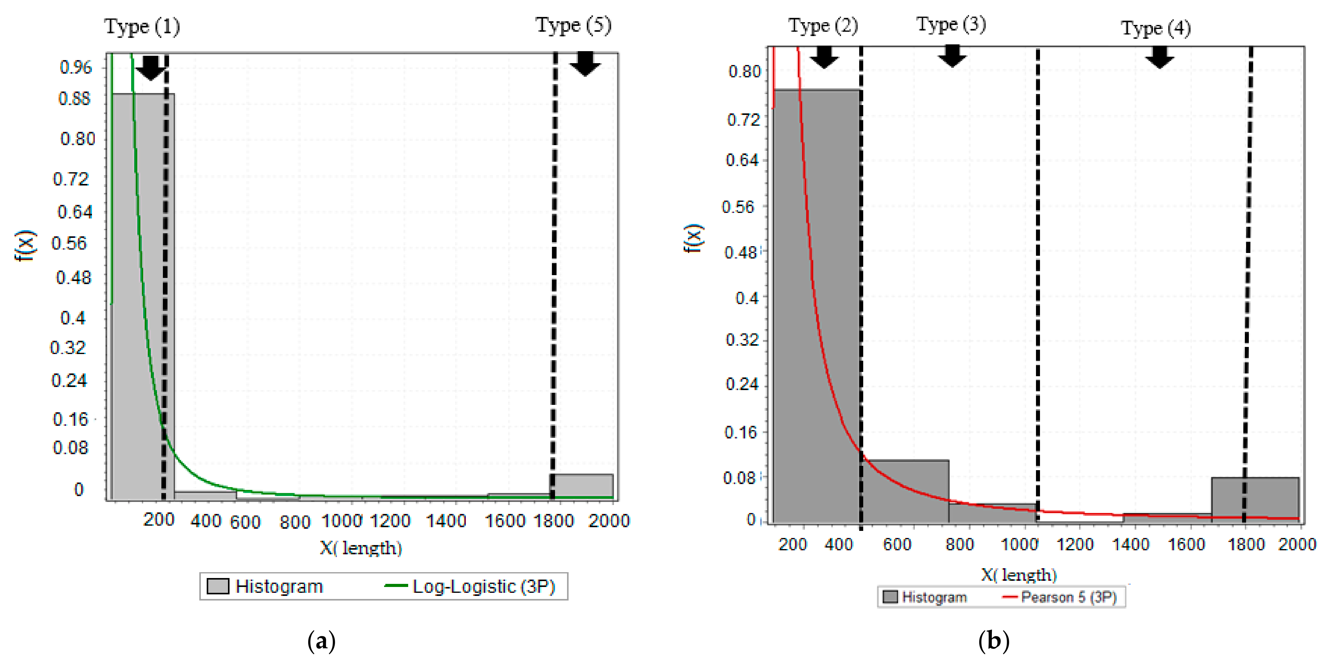
- Data classification based on the length of the signals
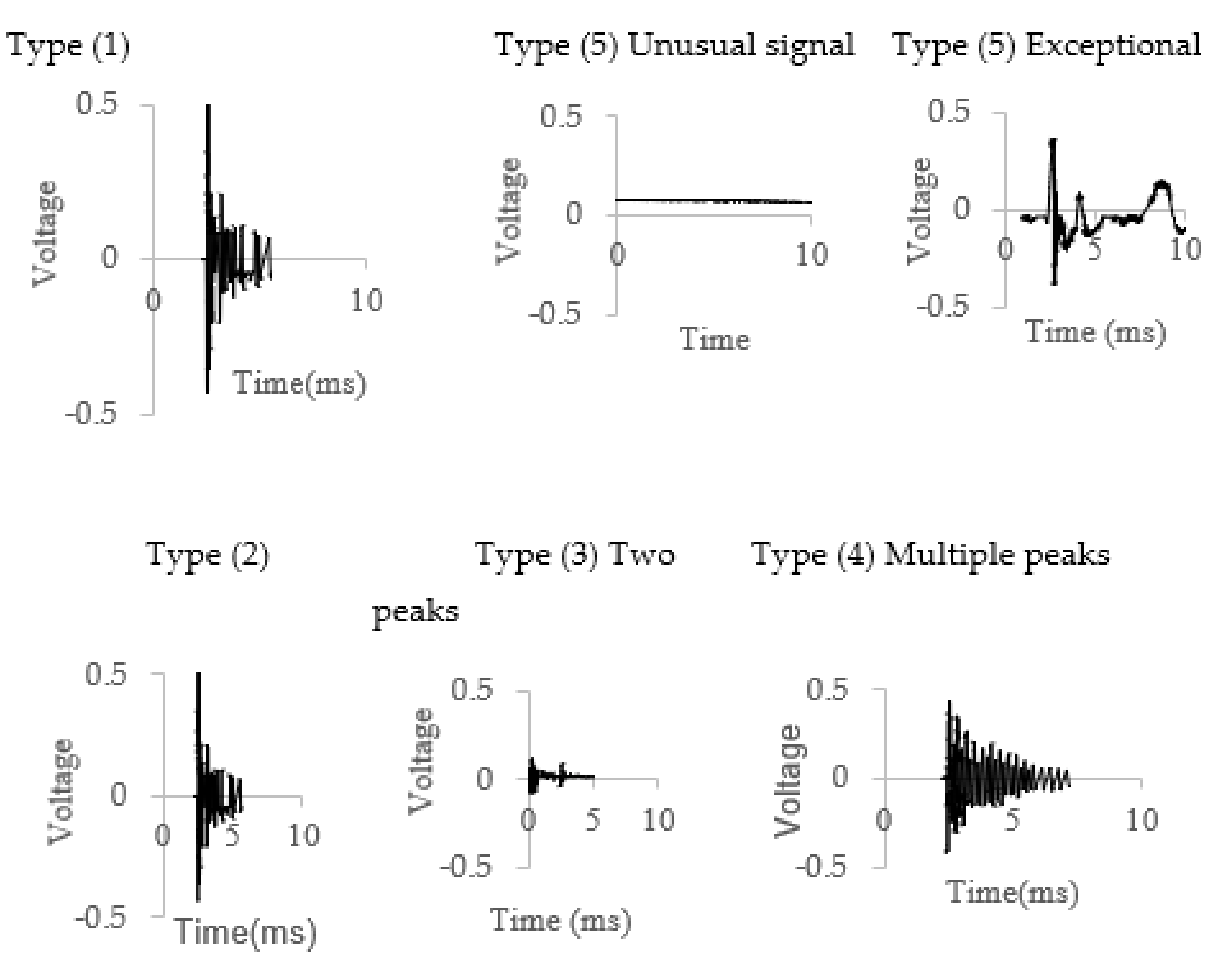
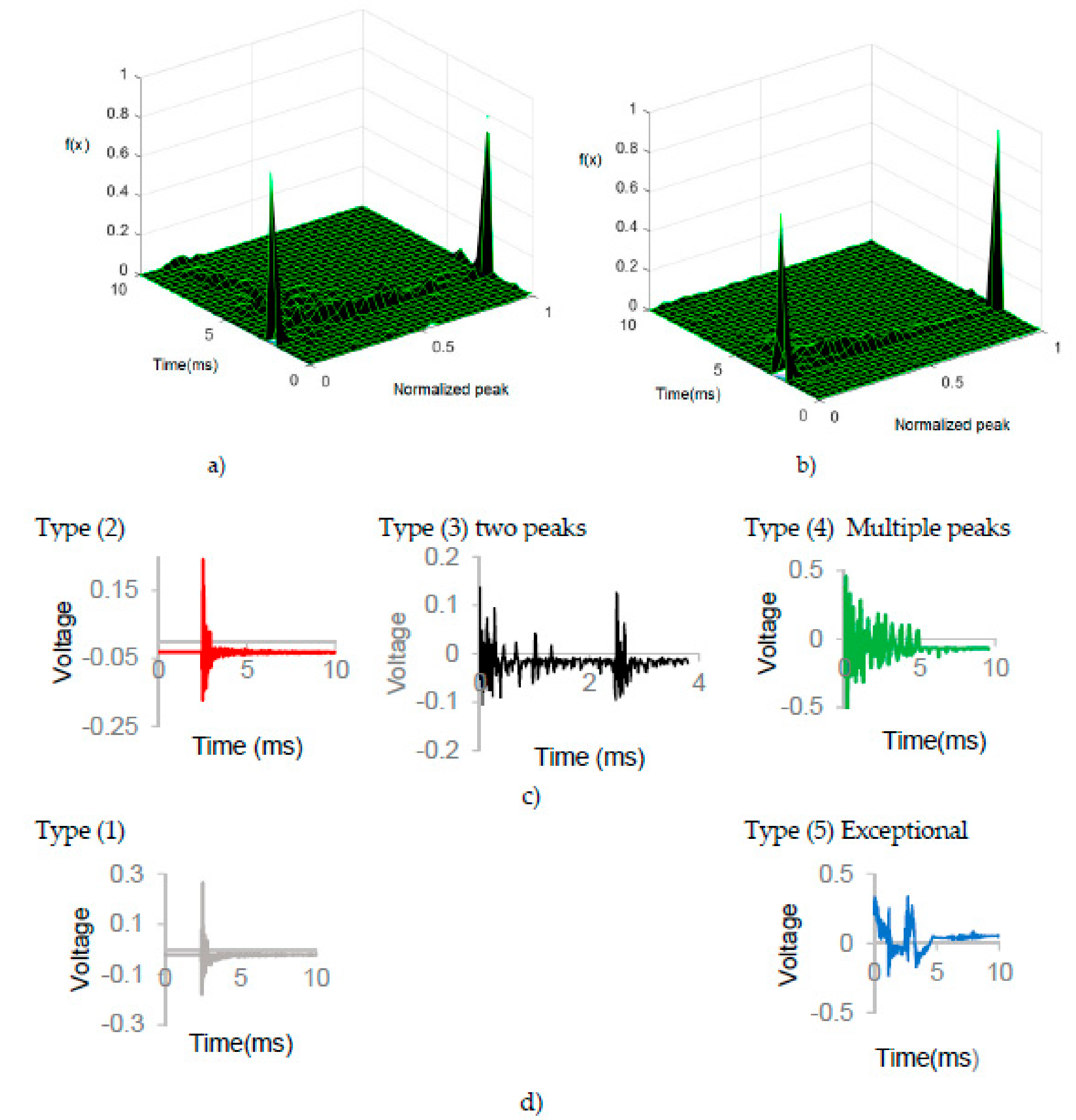
- Type (1), IE signals in sound group concluded one distinguished peak point with signal’s length contained 200 points or less.
- Type (2), IE signals in defect group concluded one or two distinguished peak points with the signal’s length contained 400 points or less than 400 points.
- Type (3), IE signals concluded one or two distinguished peaks in different times, the length of signals contained more than 400 points, and less than 1000 points.
- Type (4), IE signals concluded multiple distinguished peak points in different time intervals, the length of IE signals contained more than 1000 points, and less than 1800 points.
- Type (5), Exceptional IE signals, this type of signal broke the common pattern that was obtained by frequency analyses for classification in previous research. For example, some IE signals in the sound set were not cut by the proposed processing method due to their unusual shape.
- -
- Data classification and statistical pattern recognition based on time interval and normalized peak values.
- -
- Normalized energy
- ▪
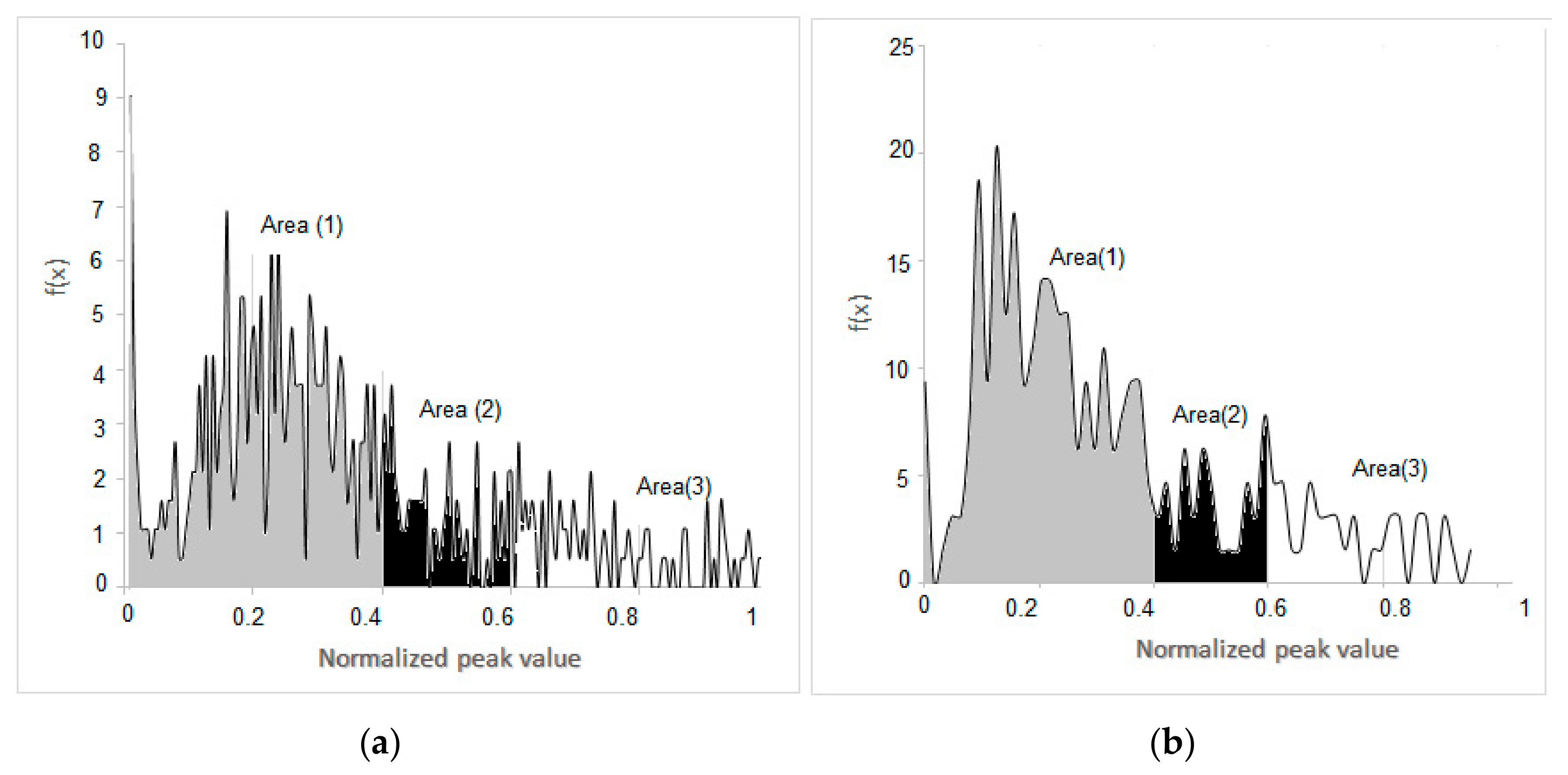
- Area 1: normalized local peaks are between 0.005 and 0.4, with small local peaks compared to the absolute maximum.
- ▪
- Area 2: normalized local peaks are between 0.4 and 0.6, with moderate local peaks compared to the absolute maximum.
- ▪
- Area 3: normalized local peaks are between 0.6 and 0.95, with significant local peaks compared to the absolute maximum.
- -
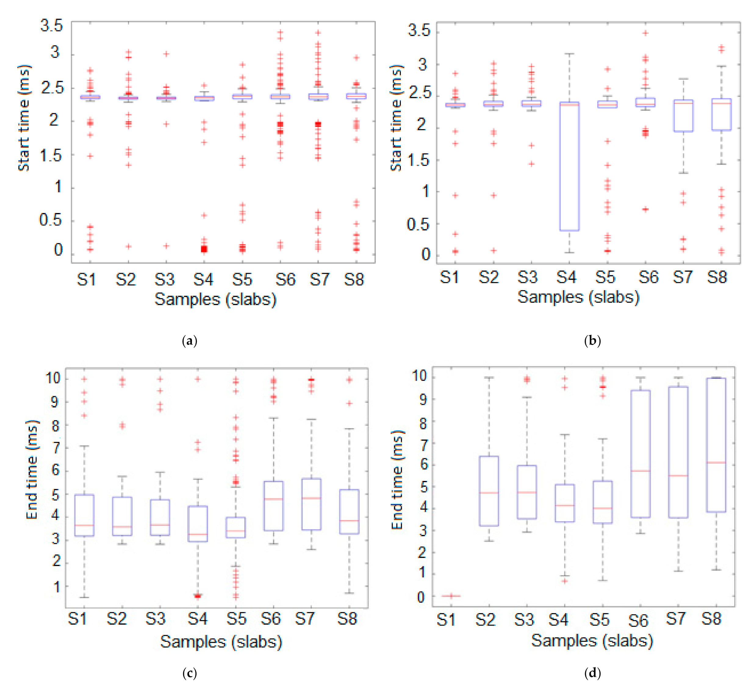
- Start and stop time
- -
- Defect type and histogram
3.2. Probability Classifier to Make Predicted Models Based on the Feature of IE Signals
- -
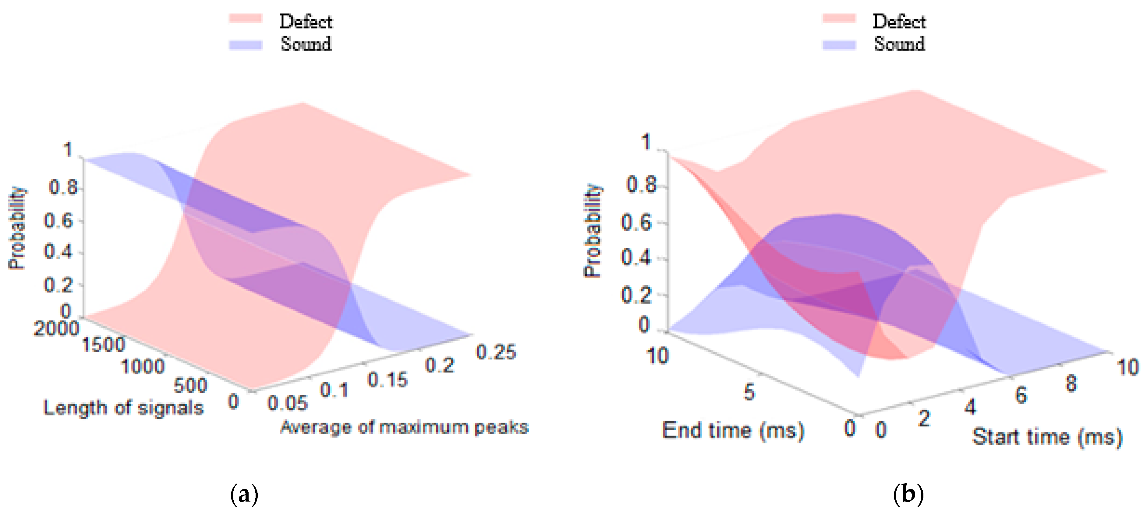
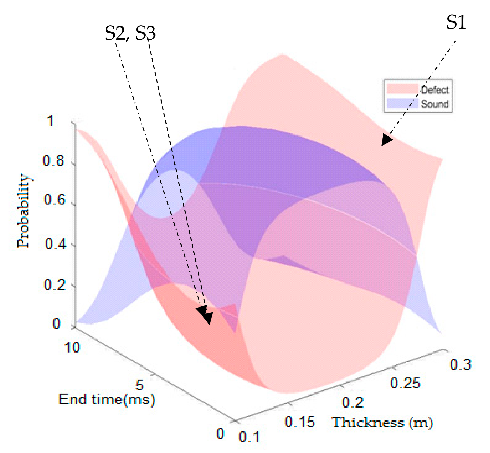
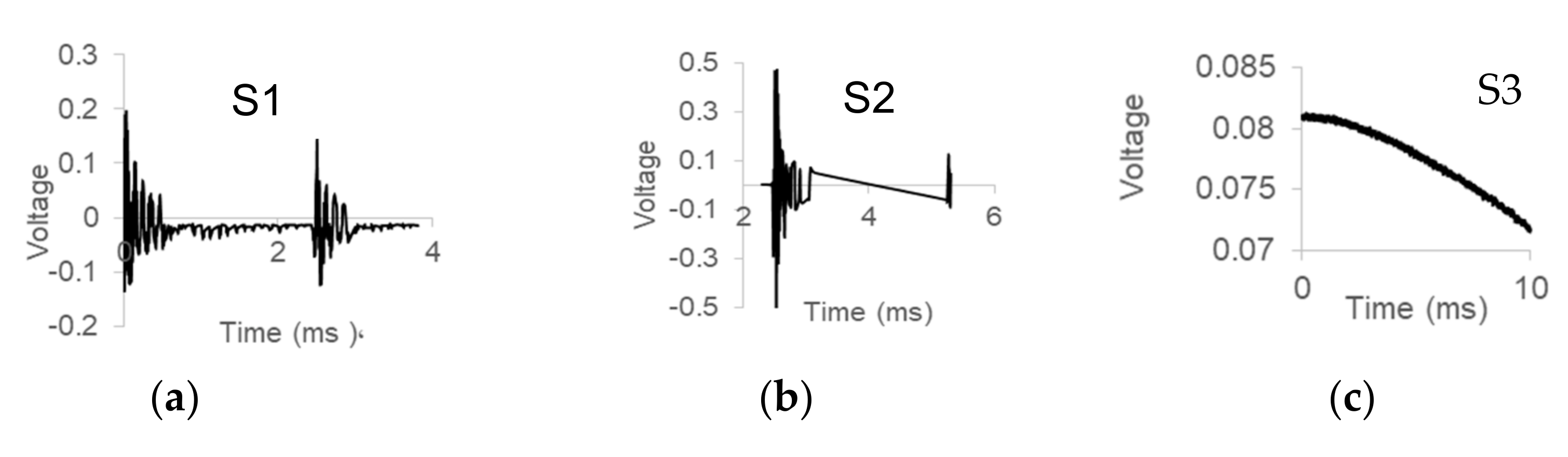
- The probability of the defect occurring ranges from 0.6–1 if the IE signal is truncated before 2 ms ().
- -
- The probability of the defect occurring ranges from 0.6–1 if the IE signal is truncated before 5 ms.
- -
- The probability that the defect occurs is between 0.8–1 if the average of maximum peak of IE signal are higher than 0.16
- -
- The probability of the defect occurring ranges from 0.1–0.2 if the IE signal is truncated between 2 and 4 ms.
- -
- The length of 90% of the preprocessed IE signals from the sound regions concluded 210 points within 2.5 and 3.5 ms. However, the length of 75% of preprocessed IE signals was concluded more than 400 points in the defect dataset, which is within 2.5 and 10 ms.
- -
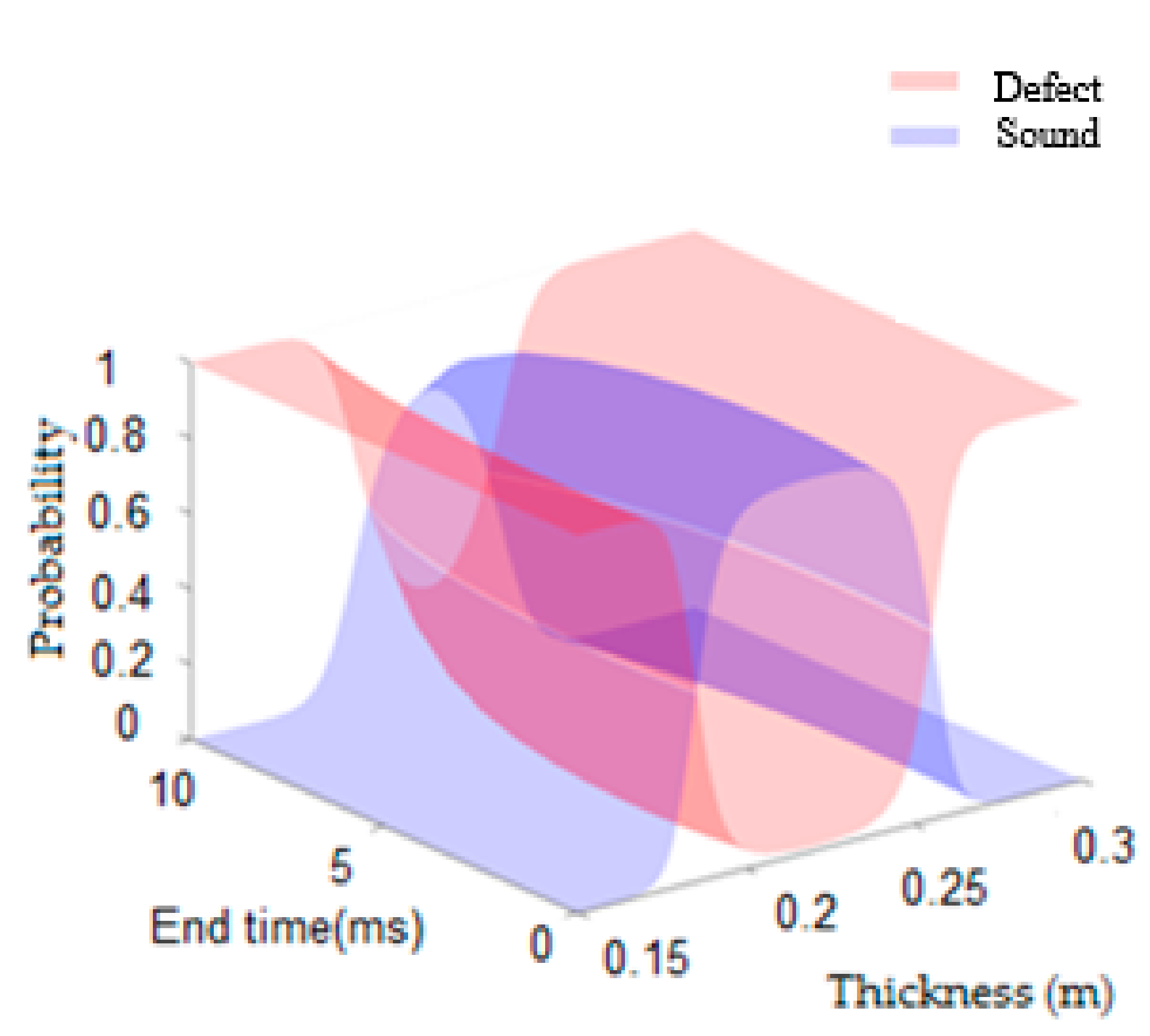
- Probability classifier to make predicted models based on the estimated thickness and end time of preprocessed IE signals
- -
- Pearson coefficient
- -
- Comparison
4. Conclusions
- -
- The result of statistical model and probability classifier shows 10% of the IE data collected from the sound area are unusable for estimating thickness using the frequency method because of unusual shape.
- -
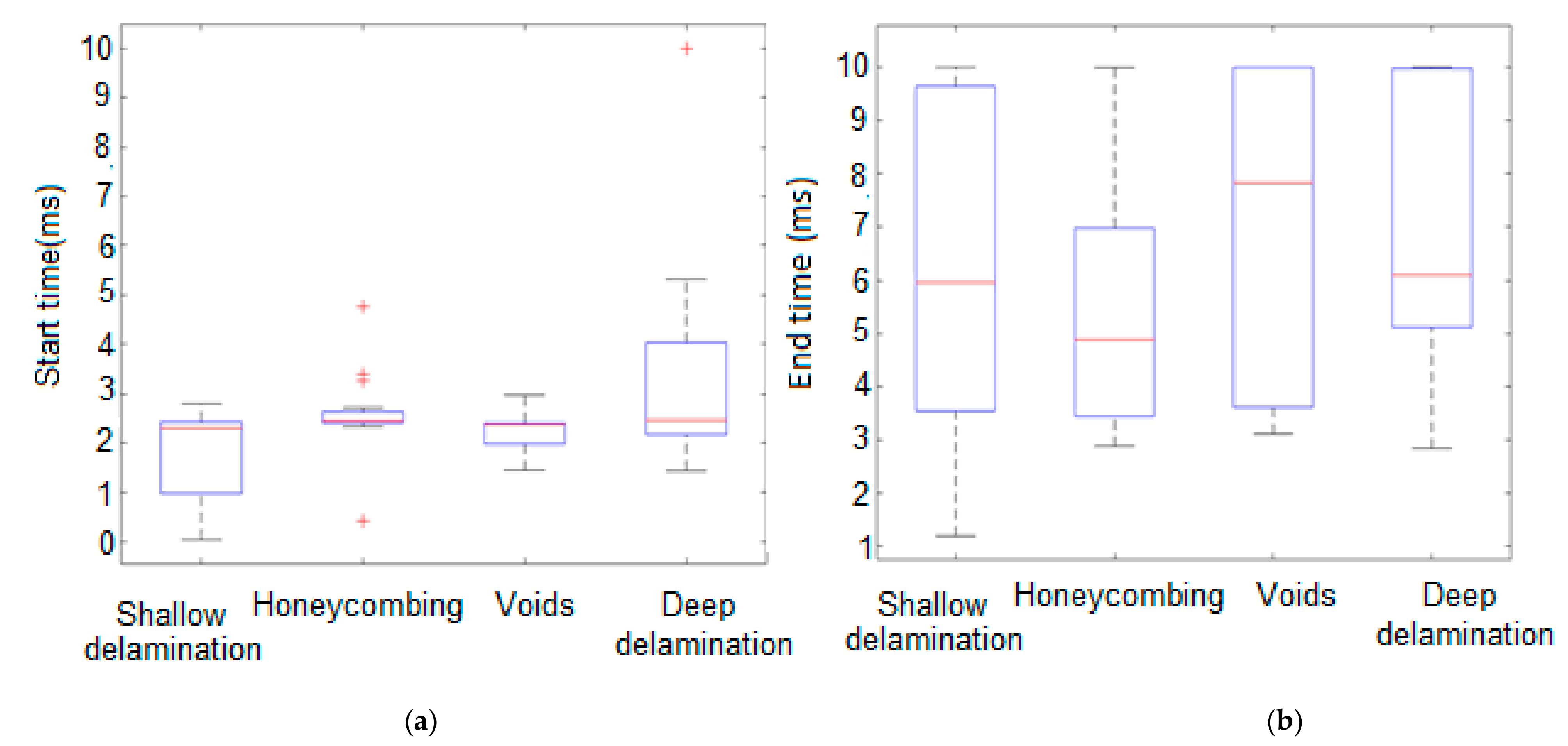
- The result over defect type of IE signals showed the detection of shallow delamination and deep delamination as defect types were more straightforward than the other two types of defect types, as 50% of the preprocessed IE data collected from shallow delamination had distinguishable points before and after 2.5 ms in the processed signals. However, the preprocessed IE signals collected from the sound area had no distinguishable peaks before 2.5 ms.
- -
- The proposed features in this study can be directly applied to IE collected by different data collection settings and devices as they were extracted from process IE signals. The result of classification using the proposed features in this study can be coupled with the conventional peak frequency method to consider both time domain and frequency domain characteristics.
- -
- Using the preprocessing approach results in obtaining more information about the number of peaks, the peak values, and the corresponding time range, which improved the classification accuracy.
- -
- Using the preprocessing approach and frequency methods leads to a better understanding of IE data, which can help the user distinguish the defect area. In addition, some data in two datasets (sound or defect) do not follow the common patterns in the dataset, which can be separated by the probability method.
- -
- With using the proposed probability, probability classifier, and preprocessing approach, it is possible to increase the rate of the frequency analyses.
Author Contributions
Funding
Institutional Review Board Statement
Informed Consent Statement
Data Availability Statement
Conflicts of Interest
References
- Ghomi, M.T.; Mahmoudi, J.; Darabi, M. Concrete plate thickness measurement using the indirect impact-echo method. Nondestruct. Test. Eval. 2013, 282, 119–144. [Google Scholar] [CrossRef]
- Edwards, L.; Bell, H.P. Comparative evaluation of nondestructive devices for measuring pavement thickness in the field. Int. J. Pavement Res. Technol. 2016, 9, 102–111. [Google Scholar] [CrossRef] [Green Version]
- Yeh, P.-L.; Liu, P.-L. Imaging of internal cracks in concrete structures using the surface rendering technique. NDT E Int. 2009, 42, 181–187. [Google Scholar] [CrossRef]
- Carino, N.J.; Sansalone, M. Flaw detection in concrete using the impact-echo method. In Bridge Evaluation, Repair and Rehabilitation; Springer: Berlin/Heidelberg, Germany, 1990; pp. 101–118. [Google Scholar]
- Kee, S.H.; Gucunski, N. Interpretation of flexural vibration modes from impact-echo testing. J. Infrastruct. Syst. 2016, 223, 04016009. [Google Scholar] [CrossRef]
- Abdelkhalek, S.; Zayed, T. Comprehensive inspection system for concrete bridge deck application: Current situation and future needs. J. Perform. Constr. Facil. 2020, 34, 03120001. [Google Scholar] [CrossRef]
- Muldoon, R.; Chalker, A.; Forde, M.C.; Ohtsu, M.; Kunisue, F. Identifying voids in plastic ducts in post-tensioning prestressed concrete members by resonant frequency of impact–echo, SIBIE and tomography. Constr. Build. Mater. 2007, 213, 527–537. [Google Scholar] [CrossRef]
- Colla, C.; Lausch, R. Influence of source frequency on impact-echo data quality for testing concrete structures. NDT E Int. 2003, 364, 203–213. [Google Scholar] [CrossRef]
- Nguyen, T.D.; Tran, K.T.; Gucunski, N. Detection of bridge-deck delamination using full ultrasonic waveform tomography. J. Infrastruct. Syst. 2017, 232, 04016027. [Google Scholar] [CrossRef]
- Yeh, P.L.; Liu, P.L.; Hsu, Y.Y. Parametric analysis of the impact-echo phase method in the differentiation of reinforcing bar and crack signals. Constr. Build. Mater. 2018, 180, 375–381. [Google Scholar] [CrossRef]
- Dorafshan, S.; Azari, H. Deep learning models for bridge deck evaluation using impact echo. Constr. Build. Mater. 2020, 263, 120109. [Google Scholar] [CrossRef]
- Schubert, F.; Wiggenhauser, H.; Lausch, R. On the accuracy of thickness measurements in impact-echo testing of finite concrete specimens––Numerical and experimental results. Ultrasonics 2004, 421, 897–901. [Google Scholar] [CrossRef]
- Schoefs, F.; Abraham, O. Probabilistic evaluation to improve design of impact–echo sources. Transp. Res. Rec. 2012, 23131, 109–115. [Google Scholar] [CrossRef] [Green Version]
- Igual, J.; Salazar, A.; Safont, G.; Vergara, L. Semi-supervised Bayesian classification of materials with impact-echo signals. Sensors 2015, 155, 11528–11550. [Google Scholar] [CrossRef]
- Pagnotta, A. Probabilistic Impact-Echo Method for Nondestructive Detection of Defects around Steel Reinforcing Bars in Reinforced Concrete. Ph.D. Thesis, Civil Engineering in the Graduate College, University of Illinois at Urbana-Champaign, Champaign, IL, USA, 2018. [Google Scholar]
- Rashidi, M.; Azari, H.; Nehme, J. Assessment of the overall condition of bridge decks using the Jensen-Shannon divergence of NDE data. NDT E Int. 2020, 110, 102204. [Google Scholar] [CrossRef]
- Ye, J.; Kobayashi, T.; Iwata, M.; Tsuda, H.; Murakawa, M. Computerized hammer sounding interpretation for concrete assessment with online machine learning. Sensors 2018, 18, 833. [Google Scholar] [CrossRef] [PubMed] [Green Version]
- Cho, Y.S.; Hong, S.U.; Lee, M.S. The assessment of the compressive strength and thickness of concrete structures using nondestructive testing and an artificial neural network. Nondestruct. Test. Eval. 2009, 243, 277–288. [Google Scholar] [CrossRef]
- Sadowski, Ł.; Hoła, J.; Czarnecki, S. Non-destructive neural identification of the bond between concrete layers in existing elements. Constr. Build. Mater. 2016, 127, 49–58. [Google Scholar] [CrossRef]
- Dorafshan, S.; Azari, H. Evaluation of bridge decks with overlays using impact echo, a deep learning approach. Autom. Constr. 2020, 113, 103133. [Google Scholar] [CrossRef]
- Zheng, Q.; Yang, M.; Yang, J.; Zhang, Q.; Zhang, X. Improvement of Generalization Ability of Deep CNN via Implicit Regularization in Two-Stage Training Process. IEEE Access 2018, 6, 15844–15869. [Google Scholar] [CrossRef]
- Shen, J.; Li, S.; Jia, F.; Zuo, H.; Ma, J. A deep multi-label learning framework for the intelligent fault diagnosis of machines. IEEE Access 2020, 8, 113557–113566. [Google Scholar] [CrossRef]
- Adam, A.; Shapiai, M.I.; Tumari, M.Z.M.; Mohamad, M.S.; Mubin, M. Feature Selection and Classifier Parameters Estimation for EEG Signals Peak Detection Using Particle Swarm Optimization. Sci. World J. 2014, 2014, 1–13. [Google Scholar] [CrossRef] [PubMed] [Green Version]
- Schittkowski, K. EASY-FIT: A software system for data fitting in dynamical systems. Struct. Multidiscip. Optim. 2002, 23, 153–169. [Google Scholar] [CrossRef]
- Friedman, J.; Hastie, T.; Tibshirani, R. The Elements of Statistical Learning; Springer Series in Statistics; Springer: New York, NY, USA, 2001; Volume 1. [Google Scholar]
- Sengupta, A.; Ilgin Guler, S.; Shokouhi, P. Interpreting Impact Echo Data to Predict Condition Rating of Concrete Bridge Decks: A Machine-Learning Approach. J. Bridge Eng. 2021, 268, 04021044. [Google Scholar] [CrossRef]
- Sutan, N.M.; Jaafar, M.S. Defect Detection of Concrete Material by Using Impact Echo Test. J. Nondestruct. Test. 2003, 8, 1–5. [Google Scholar]
- Garren, S.T. Maximum likelihood estimation of the correlation coefficient in a bivariate normal model with missing data. Stat. Probab. Lett. 1998, 38, 281–288. [Google Scholar] [CrossRef]
- Epp, T.; Svecova, D.; Cha, Y.J. Semi-Automated air-coupled impact-echo method for large-scale parkade structure. Sensors 2018, 18, 1018. [Google Scholar] [CrossRef] [PubMed] [Green Version]
- Zhang, J.K.; Yan, W.; Cui, D.M. Concrete condition assessment using impact-echo method and extreme learning machines. Sensors 2016, 16, 447. [Google Scholar] [CrossRef] [PubMed]
- Baggens, O.; Ryden, N. Systematic errors in Impact-Echo thickness estimation due to near field effects. NDT E Int. 2015, 69, 16–27. [Google Scholar] [CrossRef] [Green Version]


| Parameters | Slab 1 | Slab 2 | Slab 3 | Slab 4 | Slab 5 | Slab 6 | Slab 7 | Slab 8 | Mean |
|---|---|---|---|---|---|---|---|---|---|
| Number of data | 64 | 64 | 64 | 64 | 64 | 64 | 64 | 64 | 64 |
| Mean value | 243.9 | 361.23 | 272.53 | 215.47 | 330.8 | 837.5 | 589 | 402 | 399 |
| Coef. of Variance | 1.39 | 1.39 | 1.04 | 1.22 | 1.23 | 0.96 | 1.2 | 1.13 | 1.19 |
| Percentile 10% | 104.3 | 100.5 | 94.50 | 90 | 98 | 114.5 | 111 | 111.50 | 103.14 |
| Percentile 25% | 114.75 | 110.75 | 105 | 114.50 | 119.5 | 130.5 | 123 | 129.75 | 118.41 |
| Percentile 50% | 134 | 132 | 160 | 145 | 151.5 | 358.5 | 187 | 189.50 | 180.38 |
| Percentile 75% | 197 | 334.75 | 289.75 | 168.50 | 306.7 | 1893 | 436 | 438.25 | 497.21 |
| Percentile 90% | 464.4 | 1108 | 664.50 | 399 | 1026 | 1984 | 1638 | 1238 | 1062.1 |
| Best probabilistic fit | Gen- Extreme value | Pearson 3P | Log-logistic | wake by | Frechet 3P | Johnson SB | Pearson 3P | Burr | ----- |
| f(x) for 0–380 points | 0.86 | 0.76 | 0.82 | 0.88 | 0.80 | 0.52 | 0.72 | 0.70 | 0.755 |
| f(x) for 380–900 points | 0.12 | 0.09 | 0.16 | 0.10 | 0.09 | 0.11 | 0.14 | 0.18 | 0.122 |
| f(x) for 900–1600 point | 0 | 0.06 | 0.02 | 0.01 | 0.08 | 0.04 | 0.04 | 0.08 | 0.043 |
| f(x) for 1600–2000 point | 0.01 | 0.07 | 0 | 0.005 | 0.03 | 0.01 | 0.09 | 0.02 | 0.030 |
| f(x) for unusual type | 0.01 | 0.02 | 0 | 0.005 | 0 | 0.32 | 0.01 | 0.02 | 0.043 |
| Parameters | Slab 1 | Slab 2 | Slab 3 | Slab 4 | Slab 5 | Slab 6 | Slab 7 | Slab 8 | Mean |
|---|---|---|---|---|---|---|---|---|---|
| Number of data | 188 | 188 | 188 | 188 | 188 | 188 | 188 | 188 | 188 |
| Mean value | 262.53 | 302.95 | 155.74 | 127.83 | 262.53 | 227 | 245.31 | 122 | 216.5 |
| Coef. of Variance | 1.71 | 1.65 | 1.51 | 1.10 | 1 | 1.42 | 1.31 | 1.36 | 1.386 |
| Percentile 10% | 96 | 97 | 90.9 | 77.80 | 96 | 102 | 100.9 | 99.99 | 95.17 |
| Percentile 25% Q1 | 107.25 | 104 | 99 | 95 | 108.25 | 113 | 112.2 | 109.25 | 106.2 |
| Percentile 50% | 126 | 119.5 | 114.5 | 110 | 123 | 129 | 133 | 122.5 | 122.1 |
| Percentile 75% Q3 | 151.75 | 153.25 | 137.75 | 126.50 | 147 | 169 | 200 | 149 | 153.9 |
| Percentile 90% | 279.5 | 1359.5 | 157.70 | 149.50 | 446 | 402 | 501 | 210.40 | 441.2 |
| Best probabilistic fit | Log-logistic | Burr 4P | wake by | wake by | Cauchy | Levy 2P | Burr 4P | Burr 4P | ---- |
| f(x) for 0–250 points | 0.9 | 0.87 | 0.98 | 0.98 | 0.88 | 0.88 | 0.86 | 0.94 | 0.911 |
| f(x) for 250–900 points | 0.05 | 0.04 | 0.01 | 0.01 | 0.05 | 0.08 | 0.10 | 0.02 | 0.042 |
| f(x) for 900–2000 point | 0.02 | 0.03 | 0.002 | 0.005 | 0.06 | 0.03 | 0.02 | 0.02 | 0.024 |
| f(x) for unusual (type 6) | 0.02 | 0.05 | 0.008 | 0.005 | 0.01 | 0.01 | 0.01 | 0.01 | 0.020 |
| (a) | |||||||||
|---|---|---|---|---|---|---|---|---|---|
| Slab 1 | Slab 2 | Slab 3 | Slab 4 | Slab 5 | Slab 6 | Slab 7 | Slab 8 | Mean | |
| Number of data 64 × (number of peaks for each signal = 5) | 320 | 320 | 320 | 320 | 320 | 320 | 320 | 320 | 320 |
| f(x) for number of peaks between 0 to 2 ms | 0.05 | 0.02 | 0.67 | 0.22 | 0.13 | 0.25 | 0.07 | 0.09 | 0.21 |
| f(x) for number of peaks between 2 to 4.5 ms | 0.75 | 0.79 | 0.20 | 0.66 | 0.74 | 0.47 | 0.64 | 0.60 | 0.60 |
| f(x) for number of peaks between 4.5 to 9.99 ms | 0.20 | 0.19 | 0.13 | 0.12 | 0.11 | 0.28 | 0.13 | 0.31 | 0.19 |
| (b) | |||||||||
| Slab 1 | Slab 2 | Slab 3 | Slab 4 | Slab 5 | Slab 6 | Slab 7 | Slab 8 | Mean | |
| Number of data 188 × (number of peaks for each signal = 5) | 940 | 940 | 940 | 940 | 940 | 940 | 940 | 940 | 940 |
| f(x) for number of peaks between 0 to 2 ms | 0.03 | 0.012 | 0.005 | 0.19 | 0.07 | 0.03 | 0.07 | 0.07 | 0.06 |
| f(x) for number of peaks between 2 to 3.5 ms | 0.88 | 0.90 | 0.96 | 0.76 | 0.89 | 0.76 | 0.72 | 0.85 | 0.85 |
| f(x) for number of peaks between 3.5 to 9 ms | 0.10 | 0.10 | 0.05 | 0.06 | 0.05 | 0.22 | 0.21 | 0.06 | 0.11 |
| (a) | |||||||||
|---|---|---|---|---|---|---|---|---|---|
| Slab 1 | Slab 2 | Slab 3 | Slab 4 | Slab 5 | Slab 6 | Slab 7 | Slab 8 | Mean | |
| Number of peaks 5 × 64 | 320 | 320 | 320 | 320 | 320 | 320 | 320 | 320 | 320 |
| Area 1 | 4.19 | 4.50 | 4.30 | 4.26 | 4.74 | 4.87 | 4.85 | 4.69 | 4.55 |
| Area 2 | 0.82 | 0.74 | 0.85 | 0.85 | 0.84 | 0.62 | 0.66 | 0.98 | 0.80 |
| Area 3 | 1.42 | 1.26 | 1.23 | 1.53 | 1.17 | 1.50 | 1.37 | 1.21 | 1.33 |
| (b) | |||||||||
| Slab 1 | Slab 2 | Slab 3 | Slab 4 | Slab 5 | Slab 6 | Slab 7 | Slab 8 | Mean | |
| Number of peaks 5 × 188 | 940 | 940 | 940 | 940 | 940 | 940 | 940 | 940 | 940 |
| Area 1 | 1.50 | 1.59 | 1.54 | 1.47 | 1.56 | 1.68 | 1.65 | 1.56 | 1.57 |
| Area 2 | 0.39 | 0.25 | 0.26 | 0.26 | 0.32 | 0.24 | 0.24 | 0.32 | 0.29 |
| Area 3 | 0.41 | 0.40 | 0.42 | 0.52 | 0.46 | 0.45 | 0.48 | 0.46 | 0.45 |
| Parameters | Shallow Delamination | Honeycombing | Voids | Deep Delimitation | Mean |
|---|---|---|---|---|---|
| Number of data | 128 | 128 | 128 | 128 | 128 |
| Mean value | 551 | 330 | 380.29 | 338 | 399 |
| Coef. of Variance | 0.90 | 1.45 | 1.20 | 1.5 | 1.26 |
| Percentile 10% | 117 | 95.9 | 113.2 | 99.3 | 106 |
| Percentile 25% | 175.75 | 114.25 | 132.5 | 110.25 | 132 |
| Percentile 50% | 415 | 146.5 | 201 | 134.5 | 224 |
| Percentile 75% | 900.5 | 234 | 473 | 213 | 455 |
| Percentile 90% | 1716.25 | 1861 | 1727 | 1962 | 1816 |
| Best probabilistic fit | Fatigue life 3P | Pearson 5 3P | Burr | Logistic | ---- |
| f(x) for 0–370 points | 0.42 | 0.78 | 0.70 | 0.80 | 0.67 |
| f(x) for 370–900 points | 0.30 | 0.04 | 0.10 | 0.02 | 0.11 |
| f(x) for 900–1600 points | 0.18 | 0.01 | 0.06 | 0.02 | 0.06 |
| f(x) for 1600–2000 points | 0.52 | 0.12 | 0.11 | 0.15 | 0.22 |
| f(x) for unusual type | 0 | 0.005 | 0.03 | 0.01 | 0.0125 |
| Slab 1 | Slab 2 | Slab 3 | Slab 4 | Slab 5 | Slab 6 | Slab 7 | Slab 8 | |
|---|---|---|---|---|---|---|---|---|
| Slab 1 | 1 | 0.8437 | 0.7359 | 0.7070 | 0.4921 | 0.7891 | 0.6845 | 0.5638 |
| Slab 2 | 0.8437 | 1 | 0.7167 | 0.8763 | 0.6200 | 0.6890 | 0.8553 | 0.7167 |
| Slab 3 | 0.7359 | 0.7167 | 1 | 0.9568 | 0.6368 | 0.6559 | 0.8732 | 0.7417 |
| Slab 4 | 0.7070 | 0.8763 | 0.9568 | 1 | 0.7024 | 0.7399 | 0.8485 | 0.7926 |
| Slab 5 | 0.4921 | 0.6200 | 0.6368 | 0.7024 | 1 | 0.6442 | 0.7456 | 0.9543 |
| Slab 6 | 0.7891 | 0.6890 | 0.6559 | 0.7399 | 0.6442 | 1 | 0.6790 | 0.6710 |
| Slab 7 | 0.6845 | 0.8553 | 0.8732 | 0.8485 | 0.7456 | 0.6790 | 1 | 0.8364 |
| Slab 8 | 0.5638 | 0.7167 | 0.7417 | 0.7926 | 0.9543 | 0.6710 | 0.8364 | 1 |
Publisher’s Note: MDPI stays neutral with regard to jurisdictional claims in published maps and institutional affiliations. |
© 2021 by the authors. Licensee MDPI, Basel, Switzerland. This article is an open access article distributed under the terms and conditions of the Creative Commons Attribution (CC BY) license (https://creativecommons.org/licenses/by/4.0/).
Share and Cite
Jafari, F.; Dorafshan, S. Bridge Inspection and Defect Recognition with Using Impact Echo Data, Probability, and Naive Bayes Classifiers. Infrastructures 2021, 6, 132. https://doi.org/10.3390/infrastructures6090132
Jafari F, Dorafshan S. Bridge Inspection and Defect Recognition with Using Impact Echo Data, Probability, and Naive Bayes Classifiers. Infrastructures. 2021; 6(9):132. https://doi.org/10.3390/infrastructures6090132
Chicago/Turabian StyleJafari, Faezeh, and Sattar Dorafshan. 2021. "Bridge Inspection and Defect Recognition with Using Impact Echo Data, Probability, and Naive Bayes Classifiers" Infrastructures 6, no. 9: 132. https://doi.org/10.3390/infrastructures6090132
APA StyleJafari, F., & Dorafshan, S. (2021). Bridge Inspection and Defect Recognition with Using Impact Echo Data, Probability, and Naive Bayes Classifiers. Infrastructures, 6(9), 132. https://doi.org/10.3390/infrastructures6090132