Article

Sensitivity Investigation on the Pressure Coefficients Non-Dimensionalization

Department of Engineering and Geology, Gabriele D’Annunzio University, 65127 Pescara, Italy
Infrastructures 2021, 6(4), 53; https://doi.org/10.3390/infrastructures6040053
Submission received: 1 March 2021 / Revised: 16 March 2021 / Accepted: 31 March 2021 / Published: 1 April 2021
(This article belongs to the Special Issue Scaled Modeling for Experimental Tests)

Abstract

:
The scaling of large structures to investigate their aerodynamics in wind tunnels is a common and robust procedure to estimate important magnitudes, including pressure coefficients. Different aspects can affect the estimation of pressure coefficients; four examples are the non-dimensionalization, blockage, non-stationarity, and non-Gaussianity of the wind tunnel velocity. This paper shows the variability of pressure coefficients due to these four aspects for the case study of a closed box section of a suspended bridge. It was estimated that the pressure coefficients of similar pressure taps vary significantly due to different sets of wind velocity time history used to non-dimensionalize the wind tunnel pressures. In addition, the stationarity of the wind velocity process was not confirmed for all wind velocity sets and the non-Gaussianity of the wind velocity time history was confirmed.

1. Introduction

Error propagation due to the small scale of experimental models is known to affect results at the prototype scale [1,2,3,4,5,6]. Uncertainty related to experiments with scaled models is an issue which is currently being discussed by the international scientific community [7]. One of the causes of this uncertainty is that codes of practice do not provide experimental protocols [8,9]. In the field of structural engineering, the scaling of prototypes is commonly used for lab investigations of magnitudes such as wind loads, vibrations, and comfort conditions [10,11]. In particular, a common practice in wind engineering is to use scale models for experimental campaigns in wind tunnels.
This paper is focused on wind tunnel tests to estimate pressure coefficients. The uncertainty related to the entire process of testing affects results at the prototype scale. Several approximations should be considered. Two of these are the geometry and the simulation of the environmental conditions. The first consists of the accuracy of the test model: its geometry, the roughness of its surface, and the number of details that are represented. The second consists of the wind velocity and turbulence simulation [12,13]. In particular, the pressure coefficient is non-dimensionalized on the wind tunnel velocity. Thus, to investigate the dependence on the Reynolds number, tests are repeated using different wind tunnel velocity sets. The kinetic pressure is estimated using the mean value of a wind tunnel time history assuming that it is stationary and Gaussian. However, the mean value is not always representative of the measured random process [7] and can affect the pressure coefficient calculation.
Based on the discussion of the uncertainty [14,15,16,17,18,19] related to the non-dimensionalization of pressure coefficients [20,21], a wind tunnel experimental campaign was proposed for closed box sections of a suspended bridge [22,23,24,25] carried out with the purpose to investigate the suspended bridge instability due to the wind action [26,27,28,29,30,31,32,33,34]. Section 2 discusses the setup of the experimental tests and the experimental error estimated by observing the stationarity, the Gaussianity [35,36,37], the fluctuation of the mean and standard deviation of the wind tunnel velocity time histories, and the blockage effect [38,39,40,41,42,43,44,45,46,47]. Section 3 discusses the variability of the pressure coefficients due to non-dimensionalization.

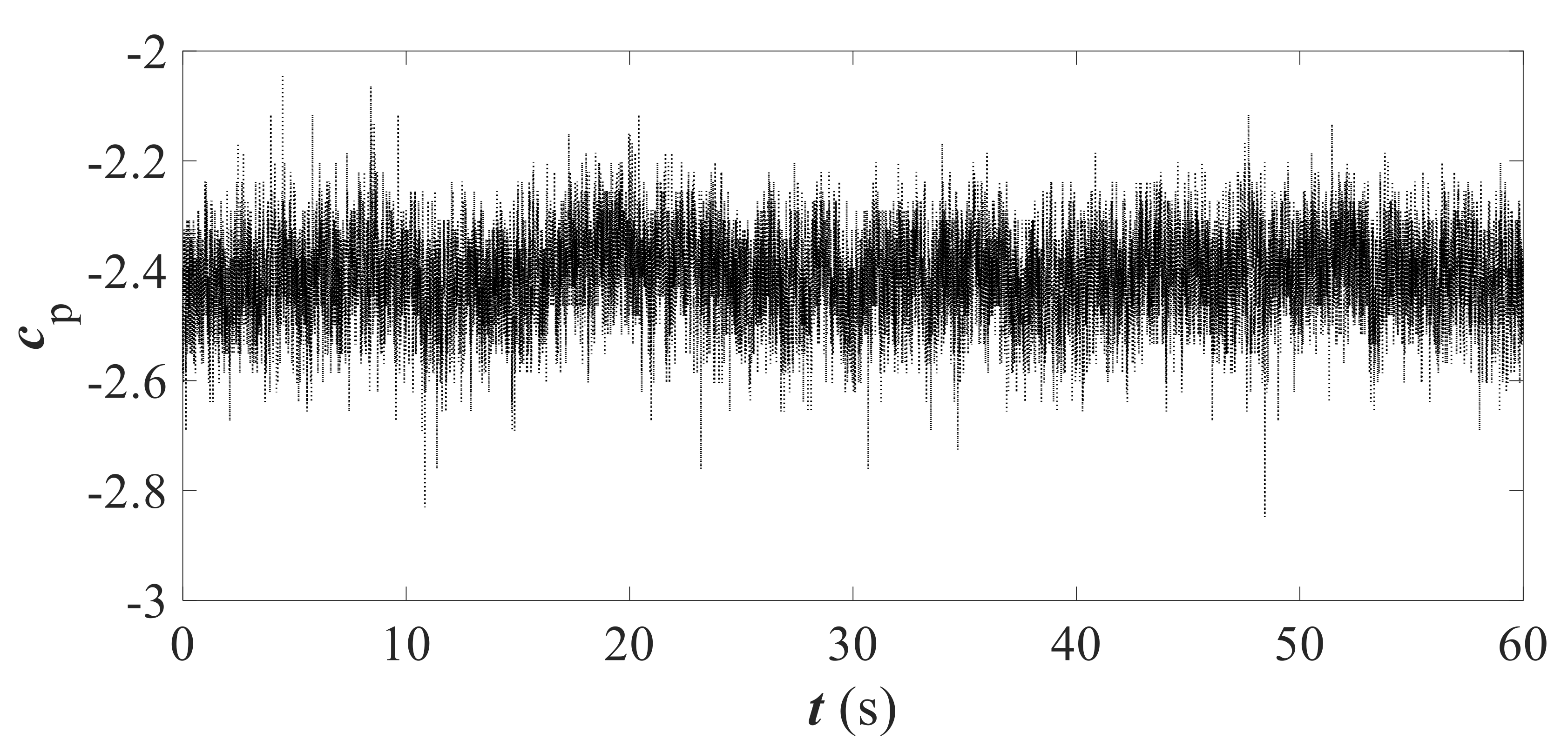
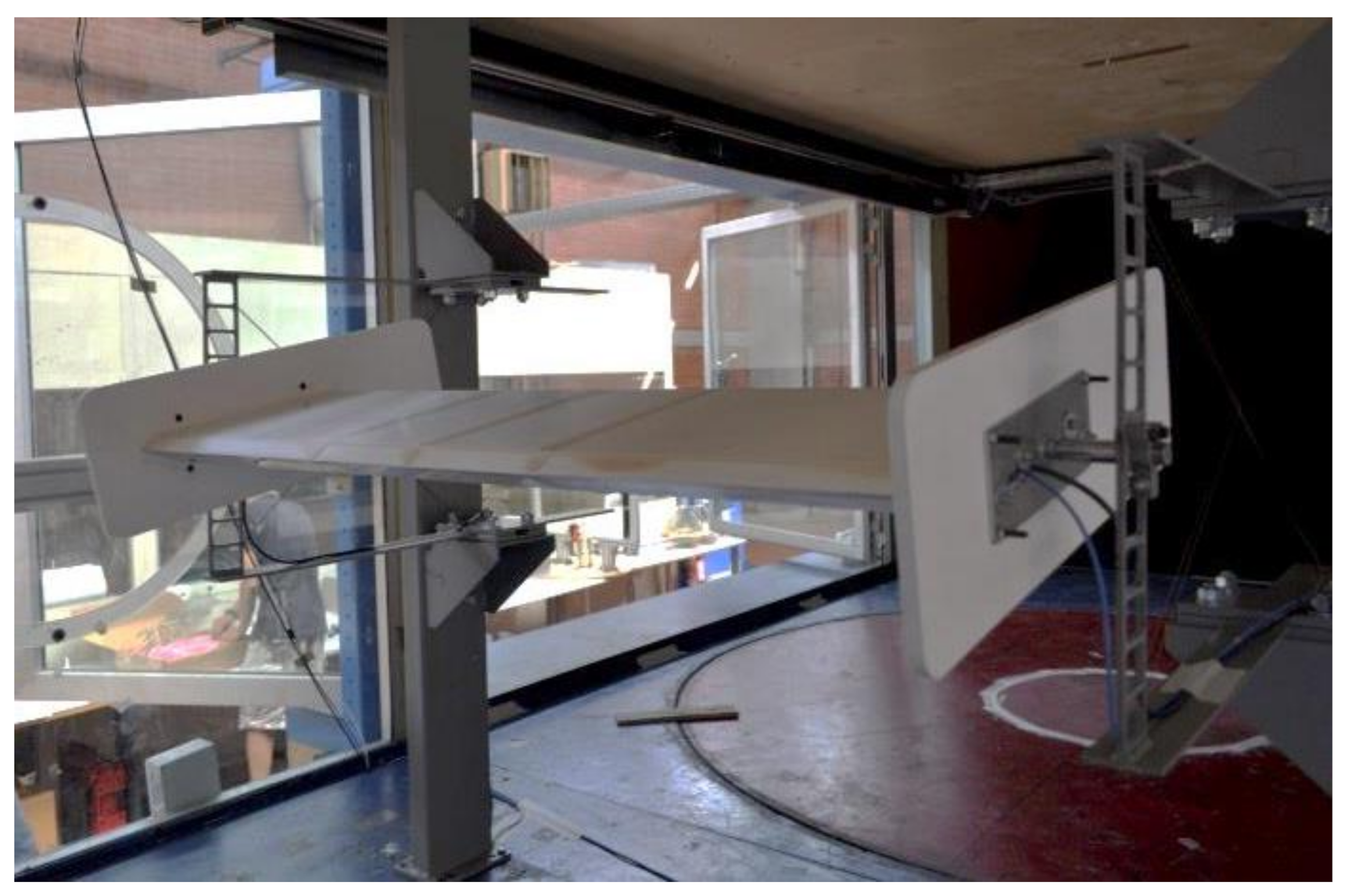
2. Wind Tunnel Experimental Setup: Pressure Random Processes

The investigation of the variability of pressure coefficients due to the wind velocity time history resulting from non-dimensionalization is discussed based on the case study of a closed box section of a suspended bridge [3]. Figure 1 shows the two geometries of the closed box section tested in a wind tunnel and discussed in this paper.
Table 1 summarizes the geometrical parameters illustrated in Figure 2 [3,22,23,24,25]. Rizzo et al. 2018 [7] discussed the trend of the mean pressure coefficients for all fifteen angles of attack tested in a wind tunnel [3].

2.1. Pressure Coefficient Estimation: Methodology

The pressure coefficients were estimated through experiments carried out in the CRIACIV (Inter-University Research Centre for Wind Engineering and Building Aerodynamics) boundary layer wind tunnel in Prato (Italy). This is an open-circuit wind tunnel with a reference test section, which is 2.42 m wide and 1.60 m high. The total length of the wind tunnel is about 22 m. The length of the test section was equal to 11.00 m. Wind speed is regulated both by adjusting the pitch of the ten-fan blades and by controlling the angular speed of the motor [3]. The maximum wind speed is about 30 m/s. The models were made of ABS (acrylonitrile butadiene styrene) and were horizontally placed in the wind tunnel. They were rigidly connected to a support system, composed of rigid arms, as illustrated in Figure 2 [3]. The sampling frequency during the tests was 497.8 Hz and the acquisition time was 60 s. The entire pressure signals contained 497.8 Hz × 60 s = 29,868 time-steps. The turbulence intensity had a mean value less than 1%.
The dimensionless pressure coefficient (Cp) time history was estimated from the difference between the static pressure measured at each pressure tap (pi) and the reference flow static pressure p0, under the wind tunnel velocity U , according to Equation (1) [3]. In Equation (1), the quantities Cp, p i , and U are time-dependent. The quantity 1 2 ρ U 2 is the kinetic pressure and depends on the air density ρ and the wind tunnel velocity U .
C p = p i   p 0 1 2 ρ U 2
In total, three strips of 40 pressure taps, placed around the cross section, were simultaneously used for three different models of a closed box section of a suspended bridge. For the sake of brevity, only two geometries are discussed in this paper. Results relating to the strip in the middle of the test section model are discussed in this paper. Fifteen angles of attack were tested in the wind tunnel: −10°, −8°, −6°, −4°, −3°, −2°, −1°, 0°, 1°, 2°, 3°, 4°, 6°, 8°, and 10°. They were investigated with the purpose to estimate the drag, lift, and moment coefficients, and, finally, to calculate the critical flutter velocity [26,27,28,29,30,31,32,33,34]. Pressure taps were connected to the pressure transducers housed inside the model, through 1.5 mm tubes made of plastic.

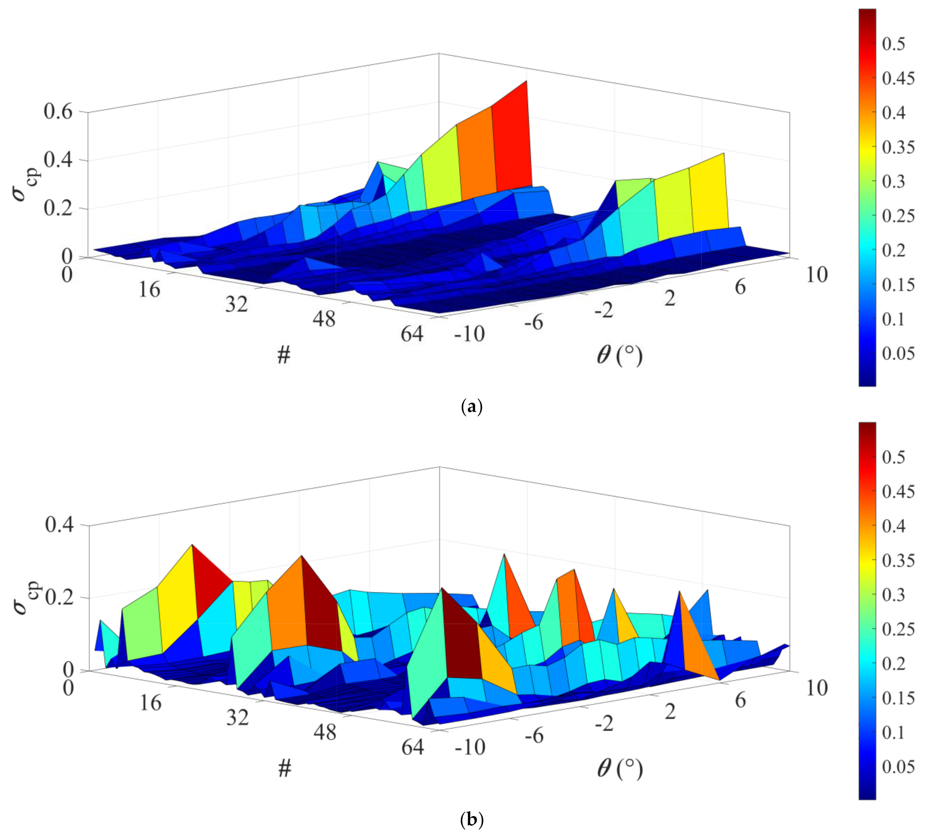
2.2. The Blockage Effect on the Pressure Coefficient

A typical experimental error occurs due to the blockage correction, which depends on both the model size and the wind tunnel test chamber section area. The blockage correction should be estimated before tests and applied to the test results.
The total blockage correction factor is defined as the sum of the velocity increment (blockage factor) caused by wake blockage and solid blockage [39]. It has long been a standard for low-speed wind tunnel testing to operate within an area ratio (i.e., tunnel cross-section to swept area of a model) of 1–10%, proposed by [39] in their text ‘‘Low-Speed Wind Tunnel Testing’’ and earlier by [40] in their text ‘‘Wind-Tunnel Technique: An Account of Experimental Methods in Low- and High-Speed Wind Tunnels’’; both provide various solid/wake blockage correction techniques.
Two types of test section are commonly used when testing in wind tunnels, namely, the closed test section and the open test section (or blockage tolerant test section), which result in large variations when referring to blockage allowances. An open test section (i.e., such as the CRIACIV wind tunnel) or open jet type of wind tunnel has the capability to allow the conditions inside the test section to be largely unaffected by larger blockage percentage static models because of the ability to leak flow and expand the flow around objects within the test section. This is in contrast to the flow constriction problem occurring in a closed test section, as shown in this study. Due to the ability to allow the flow to expand, models can generally be allowed to exhibit a higher blockage percentage in open-type testing.
Reviews of recent developments in the calculation of low-speed solid-wall wind tunnel interference were conducted by [41,42,43], and an extensive interpretation of wall pressures was detailed by [44]. According to [39], to determine the blockage corrections for wind tunnel models of unusual shapes, the following is suggested:
U = U u 1 + ε t
q = q u 1 + 2 ε t
R = R u 1 + ε t
C D 0 = C D 0 u 1 3 ε s b 2 ε w b
ε t = ε s b + ε w b = 1   m o d e l   f r o n t   a r e a 4   s e c t i o n   a r e a
where U is the velocity correction, q is the dynamic pressure correction, R is the Reynolds number correction, ε t is the blockage correction, ε s b is the solid blockage, ε w b is the wake blockage, and C D 0 is the drag coefficient correction.
Maskell (1965) [45] was the first to address the problems with non-streamlined flow bodies, such as bluff-body testing in closed wind tunnel sections and partially stalled shapes such as wings. When the high-lift characteristics of particular delta wing aircraft models with a small aspect ratio were tested in different wind tunnels at the Royal Aircraft Establishment (RAE), marked differences were observed at the onset of the stall at the wing tips, which spreading inboard with increasing incidence. The different results could be reconciled only through a wall interference factor, which is equivalent to the increase in velocity of an undisturbed stream that is much larger than previous standard estimations. Maskell’s research goal was to establish a more convincing existence of this interference factor and the need for corrections, by relating the effective increase in the dynamic pressure q of the stream due to a solid blockage constraint. Maskell’s theory holds true for nearly all two-dimensional bluff-body flows and for situations of a close-axis symmetric wake downstream for three-dimensional flows, using the equation for corrected wind velocity given below.
Alexander (1978) [46] provided an adaption to Maskell’s method by comparing the drag of flat plates normal to the freestream with the drag of Savonius rotors normal to the freestream, applying the term m . For small values of blockage ratio, S / C     = 0:045, where S is the flat plate or wind tunnel maximum frontal area, C is the wind tunnel working section cross-sectional area, and Maskell yields m = 3.15 (constant value). Alexander suggests that, due to the restriction on the wake by the tunnel walls at high S / C values, the value of m falls, reaching a value close to 2.0 for S / C = 0.3 (30% blockage).
V c 2 V 2 = 1 1 m S / C
where V c is the corrected wind velocity and V is the undisturbed wind velocity.
Lockheed scientists Hackett, Lilley, and Wilsden produced an updated blockage correction methodology [47] by adopting sources and sinks to represent an equivalent body surface in a stream. Static pressures measured at the sidewalls were used to construct a relatively simple singularity set to represent the test article and then calculate the wall effects based on that singularity set [42]. They showed that tunnel wall static pressures may be used to infer wake geometry and hence wake blockage using a row of pressures along the center of the tunnel sidewall, giving the axial distributions of both solid and wake blockages with a velocity peak just aft of the model. Through a wind tunnel testing campaign involving models of varying size and blockages up to 10%, wall pressure signatures were used to determine source, sink, and strengths with wind tunnel spans and locations. Essentially, the concept resolves pressure signatures into their solid and wake counterparts. By signifying the symmetric and anti-symmetric regions with the parameters formulated from these parts, a velocity increment expression is obtained.
Hackett and Wilsden (1975) [41] provided a theoretical method for determining wind tunnel solid/bubble and viscous blockage from wall and roof pressure measurements involving lifting and non-lifting, and powered and non-powered models. To calculate corrected pressure coefficients, they proposed:
C p = 1 C p , e m p t y C p , m o d e l 1
The blockage correction ε t was estimated according to Equation (6) and ranges from 0.25% (angle of attack equal to 0°) to 0.6% (angle of attack equal to +10° or −10°). In the case of this research, the blockage correction is very small, but contributes to the experimental error.

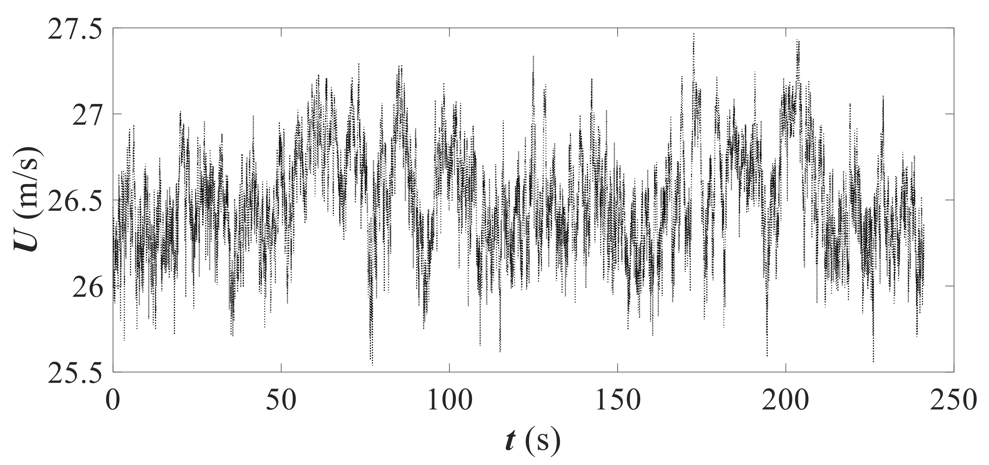
3. Wind Tunnel Experimental Setup: Wind Velocity Random Processes

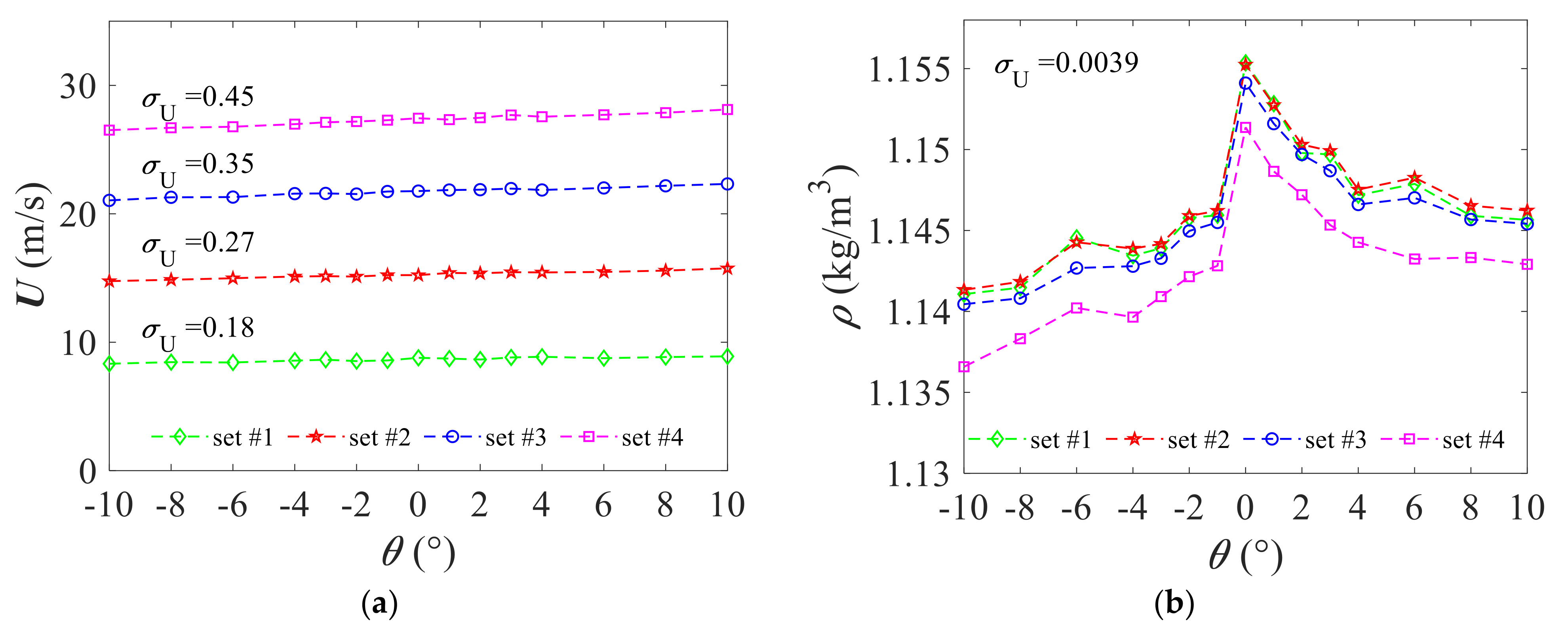
3.1. The Kinetic Pressure Variability

The kinetic pressure 1 2 ρ U 2 varies depending on both the wind velocity and the air density estimation in the wind tunnel. The wind tunnel velocity was estimated through a pitot tube before pressure tests without a model at the model position. The wind velocity is generally varied from a smaller to a bigger mean value to investigate the dependence on the Reynolds number. Commonly, the pressure acquisition is repeated using different sets of wind velocity to estimate the variation in the pressure coefficients after the pressure non-dimensionalization. Similarly, the air density is measured at every acquisition. Air density, like air pressure, decreases with increasing altitude. It also changes with variation in atmospheric pressure, temperature, and humidity.
Figure 3 shows an example of the acquired wind tunnel velocity and its random trend. In total, four sets of wind tunnel velocities are discussed here. The mean values of the wind tunnel velocities, U ¯ , were 8.33, 14.76, 21.05, and 26.52 m/s, for the angle of attack equal to −10°.
Table 2 summarizes the mean wind velocity for all angles of attack and both models. The mean value ranges from 8.33 to 8.90 m/s, from 14.76 to 15.76 m/s, from 21.05 to 22.33 m/s, and from 26.52 to 28.12 m/s, respectively. It increases from the angle of attack equal to −10° to that equal to 10°. This is not due to the aerodynamics and there is no connection to the test models. Rather, it is due to the flow stabilization in the wind tunnel after several test repetitions and because the engine was run for a long duration.
Although the above aspect may be physiological, it should be considered because the difference between the smallest (at −10°) and the biggest (at 10 °) mean values ranges from 6% to 7%. Table 2 also shows the standard deviation of the wind velocity, σ U , that ranges from 0.12 to 0.19 m/s (i.e., set #1), from 0.20 to 0.25 m/s (i.e., set #2), from 0.22 to 0.31 m/s (i.e., set #3), and from 0.22 to 0.37 m/s (i.e., set #4), respectively. The standard deviation also increases when the mean velocity increases.
The different variability calculated for each angle of attack in terms of mean and standard deviation suggests an uncertainty that should be considered by comparing pressure coefficients between different angles of attack. Figure 4a illustrates the trends shown in Table 2 and provides the standard deviation of the mean velocity considering all angles of attack, σ U θ . It was observed that the standard deviation increases linearly as a function of the mean velocity and ranges from 0.18 to 0.45 m/s.
The correct estimation of the air density in a wind tunnel can increase the experimental error. Although air density is conventionally assumed to be equal to 1.25 kg/m3, it is measured in wind tunnels before tests. Figure 4b shows the variability of the air density for all angles of attack. In this case, the air density variability is not large, and ranges from 1.36 to 1.156 kg/m3 (smaller than 2%). Air density varies for all angles of attack with a standard deviation smaller than 0.004 for both section models.
The kinetic pressure variability that considers both the air density variability and the mean wind tunnel velocity variability for each set is summarized in Table 3. It was observed that the maximum kinetic pressure varies from 13% to 15% with respect to the minimum value and generally increases from the angle of attack of −10° to 10°. As discussed previously, it does not depend on the aerodynamics but on the wind flow stabilization.

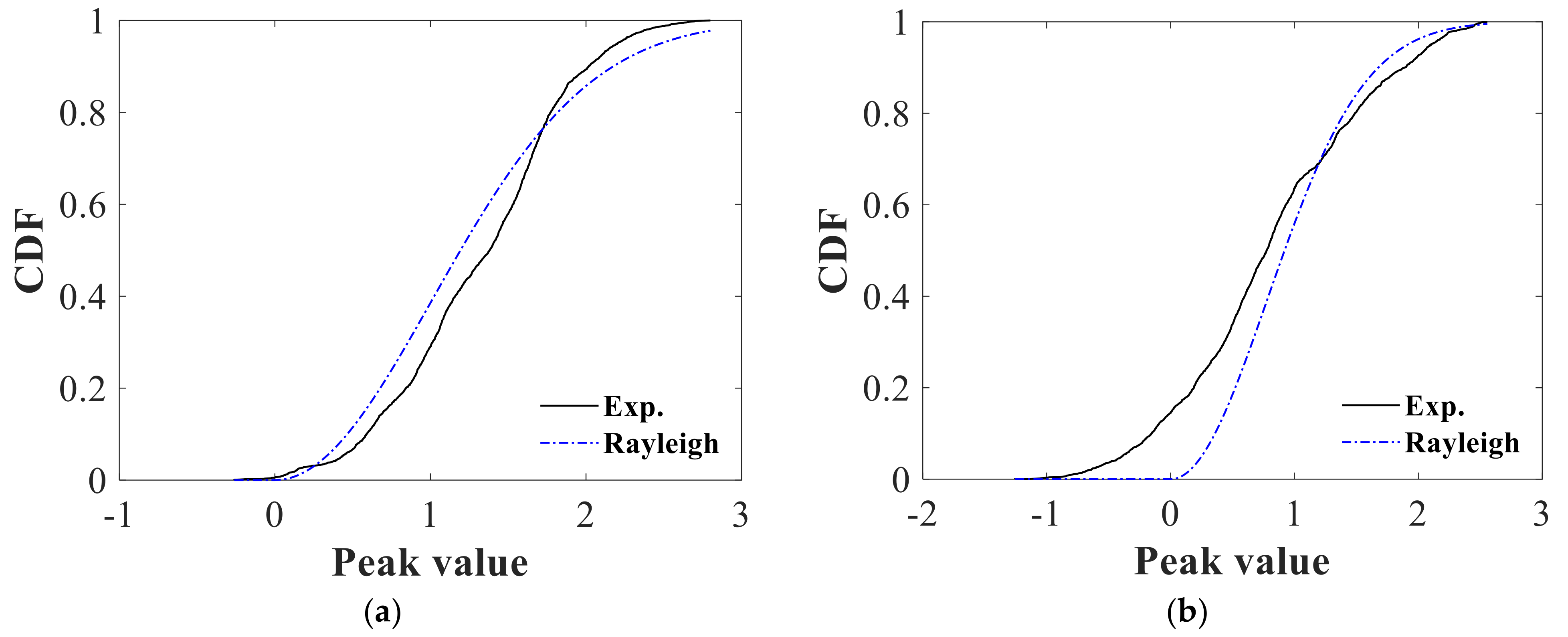
3.2. Non-Stationarity and Non-Gaussianity of the Wind Velocity Random Processes

The wind tunnel processes are commonly assumed to be stationary processes. This is generally a reliable assumption but the stationary test may not be satisfactory. If the process is not stationary, the mean value depends on the duration of the process. This aspect affects the pressure coefficient non-dimensionalization because the mean value used to estimate the kinetic pressure (Equation (1)) depends on the process duration. To measure the dependence of the mean value on the time history length, the entire time history of the wind velocity was divided into 2 s subintervals and the mean value of subintervals was calculated. The standard deviation of the mean value, σ U ¯ t i , is listed in Table 4 for all four sets of wind velocity and for all angles of attack. Values ranges from 0.08 to 0.32 m/s. Values in Table 4 can be considered negligible, but contribute to the experimental error.
Another important aspect is the Gaussianity of the wind tunnel velocity random process. The assumption that the mean value is representative of the wind tunnel velocity time history is valid only if the wind velocity random process is Gaussian. The empirical cumulative density function of the absolute peaks of the wind velocity time histories was computed and fitted using a Rayleigh distribution. If the Rayleigh distribution fits the absolute peaks, the process can be assumed to be Gaussian [35]. The one-sample Kolmogorov–Smirnov (K-S) test [7,36] at the 95% level of confidence was used to estimate the goodness of the fit. The test result h is 1 if the test rejects the null hypothesis at the 5% significance level, or 0 otherwise. Figure 5 shows two examples of the empirical Cumulative Density Function (CDF) of the normalized and standardized wind velocity local peaks fitted by the Raileigh distribution. Although the fit appears to be better in some cases (Figure 5a) than others (Figure 5b), the K-S test rejects the null hypothesis at the 5% significance level [36]. This is the same reduction in the percentage of the level of confidence.
It was concluded that the processes of wind velocities can be not defined as Gaussian and that the mean value of the wind velocity is not representative of the entire time history. This uncertainty increases the experimental error because the mean value of the wind velocity time history is assumed to affect the pressure coefficient non-dimensionalization, as given by Equaiton (1). According to [37], the non-Gaussian processes are identified by skewness greater than 0.5 and/or excessive kurtosis greater than 0.5. Table 5 shows the processes identified as Gaussian (index = 0) or non-Gaussian (index=1) according to [37]. It was observed that using this method, the number of non-Gaussian processes represented 28% of the total.

4. Remarks

A typical time history of the pressure coefficient, c p , is illustrated in Figure 6. This is a random process and is generally non-Gaussian in the detachment zones [7]. The pressure coefficient is obtained according to Equation (1) and depends on a non-dimensionalization with respect to the kinetic pressure 1 / 2 ρ U 2 . The uncertainty related to the kinetic pressure in terms of four different aspects—namely, wind velocity variability between different angles of attack, wind velocity random process non-stationarity, wind velocity random process non-Gaussianity, and air density variability—affects the pressure coefficient estimation.
It is well known that the Reynolds number can affect the pressure coefficients, and the dependence between pressure coefficients and the Reynold number should be carefully checked during the experimental campaign. The uncertainty previously discussed is often neglected because the wind velocity variability is considered to be physiological, and a small variability of the pressure coefficient is assumed to be negligible because the prototype scale is meaningless. The author of the current study agrees with this assumption; however, it should not be assumed a priori. The investigation of the dependence of the pressure coefficient on the kinetic pressure variability should entail a systematic approach to evaluate the results of the variability at the prototype scale.
The mean pressure coefficient was estimated through the non-dimensionalization using the mean wind velocity sets listed in Table 2 and by the air density given in Figure 5, for all angles of attack and both section models. In total, four pressure coefficient values were calculated for all pressure taps and the standard deviation of these four values, σ c p , was assumed as a measure of the mean pressure coefficient variability due to the non-dimensionalization. The standard deviation is plotted in Figure 7 versus the angle of attack and for all pressure taps, for Mod01 (Figure 7a) and Mod02 (Figure 7b). It was observed that the aerodynamics of the section model and the angle of attack closely affect the σ c p .
For Mod01 (Figure 2a), the standard deviation increases for most of the pressure taps from the angle of attack equal to −10° to 10°. For most pressure taps, the standard deviation ranges from 0.02 to about 0.1, whereas for 8% of the pressure taps, it ranges from 0.03 to 0.5. The last value is significant because the mean pressure coefficient for these pressure taps for the angle of attack equal to 10° is around −3.46. This means that, based on the wind tunnel velocity set chosen to non-dimensionalize the pressure, the pressure coefficient for this specific pressure tap and this specific angle of attack can vary by 14.5%.
For Mod02 (Figure 2b), the biggest value of the standard deviation is at −10° and is equal to about 0.3. On average, the standard deviation value for geometry Mod02 is bigger than that of Mod01, and is between 0.1 and 0.15. Results show that the variability is relevant for some pressure taps and depends on the geometry that affects the aerodynamics. For this reason, the variability should be investigated because it is unknown prior to testing. The consequence of this variability on the structural sizing can be negligible. An example is the sizing of the metal connections between the deck plate made of reinforced concrete and the supports made of steel. These metal connections are sized based on the shear force due to the wind force horizontal component. The wind force horizontal component is estimated using the local pressure coefficients in the detachment zone that are generally the biggest. The local pressure coefficients are values in a small area and their variability can closely affect the structural design. As estimated for the discussed case study, a variation of 15% of the pressure coefficient can be assumed as a variation of 15% of the wind force at a local scale [8]. This variation is not negligible because it can lead to an underestimation of the connection cross-section. As the bridge cross-section tested in the wind tunnel is assumed to be representative of an entire bridge cross-section that is very long, this underestimation can have serious consequences.

5. Conclusions

The experimental error related to the estimation of pressure coefficients was investigated based on a case study of a closed box section of a suspended bridge. It was observed that they are at least four different sources of uncertainty to consider.
These are:
  • The uncertainty related to different sets of wind velocity used to non-dimensionalize the pressure coefficient.
  • The uncertainty related to the stationary assumption of the wind tunnel velocity time history.
  • The uncertainty related to the Gaussianity of the wind tunnel velocity time history.
  • The uncertainty related to the blockage estimation.
It was observed that, for the case study discussed here, the mean and standard deviation of the wind velocity were not constant for all angles of attack investigated in a wind tunnel, and that the wind tunnel velocity time history could not be assumed to be entirely stationary and Gaussian. Finally, the blockage correction was estimated to be equal to a maximum of 0.6%, which was negligible in this case.
These sources of uncertainty affect the pressure coefficient and, consequently, the estimated wind action at the prototype scale. This aspect is neglected by codes and standards, but is largely discussed in the scientific literature. For the case study investigated here, the variability due to the wind velocity used to non-dimensionalize the pressure coefficient was around 15%.

Funding

This research received no external funding.

Institutional Review Board Statement

Not applicable.

Informed Consent Statement

Not applicable.

Data Availability Statement

Not applicable.

Conflicts of Interest

The author declares no conflict of interest.

References

  1. Rizzo, F.; Ricciardelli, F.; Maddaloni, G.; Bonati, A.; Occhiuzzi, A. Experimental error analysis of dynamic properties for a reduced-scale high-rise building model and implications on full-scale behavior. J. Build. Eng. 2020, 28, 101067. [Google Scholar] [CrossRef]
  2. Rizzo, F.; Caracoglia, L. Examining wind tunnel errors in Scanlan derivatives and flutter speed of a closed-box. J. Wind Struct. 2018, 26, 231–251. [Google Scholar]
  3. Rizzo, F.; Caracoglia, L.; Montelpare, S. Predicting the flutter speed of a pedestrian suspension bridge through examination of laboratory experimental errors. Eng. Struct. 2018, 172, 589–613. [Google Scholar] [CrossRef]
  4. Desceliers, C.; Soize, C.; Ghanem, R. Identification of chaos representations of elastic properties of random media using experimental vibration tests. Comput. Mech. 2007, 39, 831–838. [Google Scholar] [CrossRef]
  5. Schoefs, F.; Yáñez-Godoy, H.; Lanata, F. Polynomial chaos representation for identification of mechanical characteristics of instrumented structures. Comput. Aided Civ. Infrastruct. 2011, 26, 173–189. [Google Scholar] [CrossRef]
  6. Seo, D.W.; Caracoglia, L. Derivation of equivalent gust effect factors for wind loading on low-rise buildings through Database-Assisted-Design approach. Eng. Struct. 2010, 32, 328–336. [Google Scholar] [CrossRef]
  7. Rizzo, F.; Barbato, M.; Sepe, V. Peak factor statistics of wind effects for hyperbolic paraboloid roofs. Eng. Struct. 2018, 173, 313–330. [Google Scholar] [CrossRef]
  8. CNR. Guide for the Assessment of Wind Actions and Effects on Structures; CNR-DT; National Research Council of Italy: Rome, Italy, 2010. [Google Scholar]
  9. CEN. Eurocode 1: Actions on Structures–Part 1-4: General Actions–Wind Actions, EN-1991-1-4; Comité Européen de Normalization: Brussels, Belgium, 2008. [Google Scholar]
  10. Isyumov, N. The Aeroelastic Modelling of Tall Buildings. In International Workshop on Wind Tunnel Modelling Criteria and Technique in Civil Engineering Applications; Reinhold, T., Ed.; Cambridge University Press: Cambridge, UK, 1982. [Google Scholar]
  11. Rizzo, F.; Kopp, A.G.; Giaccu, G. Investigation of wind-induced dynamics of a cable net roof with aeroelastic wind tunnel tests. Eng. Struct. 2021, 229, 111569. [Google Scholar] [CrossRef]
  12. Barlow, J.B.; Rae, W.H.; Pope, A. Low-Speed Wind Tunnel Testing, 3rd ed.; John Wiley and Sons: New York, NY, USA, 2018. [Google Scholar]
  13. Bartoli, G.; Mannini, C. Reliability of bridge deck flutter derivative measurement in wind tunnel tests. In Proceedings of the ICOSSAR, Shangai, China, 21–25 June 2005. [Google Scholar]
  14. Ghanem, R.; Spanos, P.D. Stochastic Finite Elements: A Spectral Approach; Springer-Verlag: New York, NY, USA, 1991. [Google Scholar]
  15. Gimsing, N.J.; Georgakis, C.T. Cable Supported Bridges: Concept and Design, 3rd ed.; Wiley: Chichester, UK, 2011. [Google Scholar]
  16. Kwon, S.-D. Uncertainty of bridge flutter velocity measured at wind tunnel tests. In Proceedings of the 5th International Symposium on Computational Wind Engineering (CWE2010), Chapel Hill, NC, USA, 23–25 May 2010. [Google Scholar]
  17. Jakobsen, J.B.; Tanaka, H. Modelling uncertainties in prediction of aeroelastic bridge behaviour. J. Wind Eng. Ind. Aerodyn. 2003, 91, 1485–1498. [Google Scholar] [CrossRef]
  18. Le Maître, O.P.; Knio, O.M. Spectral Methods for Uncertainty Quantification; Springer: Berlin/Heidelberg, Germany, 2010. [Google Scholar]
  19. Mannini, C.; Bartoli, G. The problem of uncertainty in the measurement of aerodynamic derivatives. Safety, Reliability and Risk of Structures. Infrastruct. Eng. Syst. 2010, 824–831. [Google Scholar]
  20. Ricciardelli, F.; Hangan, H. Pressure distribution and aerodynamic forces on stationary box bridge sections. Wind Struct. 2001, 4, 399–412. [Google Scholar] [CrossRef]
  21. Ricciardelli, F.; de Grenet, E.T.; Hangan, H. Pressure distribution, aerodynamic forces and dynamic response of box bridge sections. J. Wind Eng. Ind. Aerodyn. 2002, 90, 1135–1150. [Google Scholar] [CrossRef]
  22. Reinhold, T.A.; Brinch, M.; Damsgaard, A. Wind tunnel tests for the Great Belt Link. In Aerodynamics of Large Bridges, Proceedings of the 1st International Symposium on Aerodynamics of Large Bridges, Copenhagen, Denmark, 19–21 February 1992; Larsen, A., Ed.; CRC Press: Boca Raton, FL, USA, 1992; ISBN 905410 042 7. [Google Scholar]
  23. Scotta, R.; Lazzari, M.; Stecca, E.; Cotela, J.; Rossi, R. Numerical wind tunnel for aerodynamic and aeroelastic characterization of bridge deck sections. Comput. Struct. 2016, 167, 96–114. [Google Scholar] [CrossRef]
  24. Rizzo, F.; Caracoglia, L. Artificial Neural Network model to predict the flutter velocity of suspension bridges. Comput. Struct. 2020, 233, 1062362020. [Google Scholar] [CrossRef]
  25. Rizzo, F.; D’Alessandro, V.; Montelpare, S.; Giammichele, L. Computational study of a bluff body aerodynamics: Impact of the laminar-to-turbulent transition modelling. Int. J. Mech. Sci. 2020, 178, 105620. [Google Scholar] [CrossRef]
  26. Jones, N.P.; Scanlan, R.H. Theory and full-bridge modeling of wind response of cable-supported bridges. J. Bridge Eng. 2001, 6, 365–375. [Google Scholar] [CrossRef]
  27. Lau, C.K.; Wong, K.Y. Aerodynamic stability of Tsing Ma Bridge. In Proceedings of the Fourth International Kerensky Conference on Structures in the New Millennium, Hong Kong, China, 3–5 September 1997. [Google Scholar]
  28. Matsumoto, M.; Kobayashi, Y.; Shirato, H. The influence of aerodynamic derivatives on flutter. J. Wind Eng. Ind. Aerodyn. 1996, 60, 227–239. [Google Scholar] [CrossRef]
  29. Ostenfeld-Rosenthal, P.; Madsen, H.O.; Larsen, A. Probabilistic flutter criteria for long span bridges. J. Wind Eng. Ind. Aerodyn. 1992, 42, 1265–1276. [Google Scholar] [CrossRef]
  30. Sarkar, P.P.; Caracoglia, L.; Haan, F.L.; Sato, H.; Murakoshi, J. Comparative and sensitivity study of flutter derivatives of selected bridge deck sections. Part 1: Analysis of inter-laboratory experimental data. Eng. Struct. 2009, 31, 158–169. [Google Scholar] [CrossRef]
  31. Scanlan, R.H.; Tomko, J.J. Airfoil and bridge deck flutter derivatives. J. Eng. Mech. 1971, 97, 1717–1737. [Google Scholar]
  32. Scanlan, R.H.; Jones, N.P. Aeroelastic analysis of cable-stayed bridges. J. Struct. Eng. 1990, 116, 279–297. [Google Scholar] [CrossRef]
  33. Scanlan, R.H.; Jones, N.P.; Singh, L. Inter-relations among flutter derivatives. J. Wind Eng. Ind. Aerodyn. 1997, 69–71, 829–837. [Google Scholar] [CrossRef]
  34. Simiu, E.; Scanlan, R.H. Wind Effects on Structures: Fundamentals and Applications to Design, 3rd ed.; John Wiley: New York, NY, USA, 1996. [Google Scholar]
  35. Davenport, A.G. Note on the distribution of the largest value of a random function with application to gust loading. Inst. Civ. Eng. 1964, 28, 187–196. [Google Scholar] [CrossRef]
  36. Massey, F.J. The Kolmogorov-Smirnov test for goodness of fit. J. Am. Stat. Assoc. 1951, 46, 68–78. [Google Scholar] [CrossRef]
  37. Suresh Kumar, K.; Stathopoulos, T. Wind loads on low building roofs: A stochastic perspective. J. Struct. Eng. 2000, 126, 944–956. [Google Scholar] [CrossRef]
  38. Ross, I.; Altman, A. Wind tunnel blockage corrections: Review and application to Savonius vertical-axis wind turbines. J. Wind Eng. Ind. Aerodyn. 2011, 99, 523–538. [Google Scholar] [CrossRef]
  39. Pope, A.; Harper, J.J. Low Speed Wind Tunnel Testing; John Wiley and Sons: New York, NY, USA, 1996. [Google Scholar]
  40. Pankhurst, R.C.; Holder, D.W. Wind-Tunnel Technique: An Account of Experimental Methods in Low-and High-Speed Wind Tunnels; Pitman: London, UK, 1952. [Google Scholar]
  41. Hackett, J.E.; Wilsden, D.J. Determination of low speed wake blockage corrections via tunnel wall static pressure measurements. In Proceedings of the AGARD Fluid Dynamic Panel Symposium on Wind tunnel Design and Testing Techniques, London, UK, 6–8 October 1975. [Google Scholar]
  42. Hackett, J.E.; Lilley, D.E.; Wilsden, D.J. Estimation of Tunnel Blockage from Wall Pressure Signatures: A Review and Data Correlation; NASA CR-15 224; Lockheed-Georgia Co: Calabasas, CA, USA, 1979. [Google Scholar]
  43. Hackett, J.E. Recent developments in the calculation of low-speed solidwalled wind tunnel wall interference in tests on large models part I: Evaluation of three interference assessment methods. Prog. Aerosp. Sci. 2003, 39, 537–583. [Google Scholar] [CrossRef]
  44. Ashill, P.R.; Weeks, D.J. A Method of Determining Wall Interference Corrections in Solid-Wall Tunnels from Measurements of Static Pressure at the Walls; AGARD-CP-335; Nato: Washington, DC, USA, 1982. [Google Scholar]
  45. Maskell, E.C. A Theory of the Blockage Effects on Bluff Bodies and Stalled Wings in a Closed Wind Tunnel; ARC R and M 3400; The Stationery Office: London, UK, 1965. [Google Scholar]
  46. Alexander, A.J. Wind tunnel corrections for Savonius rotors. In Proceedings of the Second International Symposium on Wind Energy Systems, Paper E6, Amsterdam, The Netherlands, 3–6 October 1978; pp. 69–80. [Google Scholar]
  47. Hensel, R.W. Rectangular-wind-tunnel blocking corrections using the velocity ratio method. In NACA TN 2372; NACA: Washington, DC, USA, 1951. [Google Scholar]
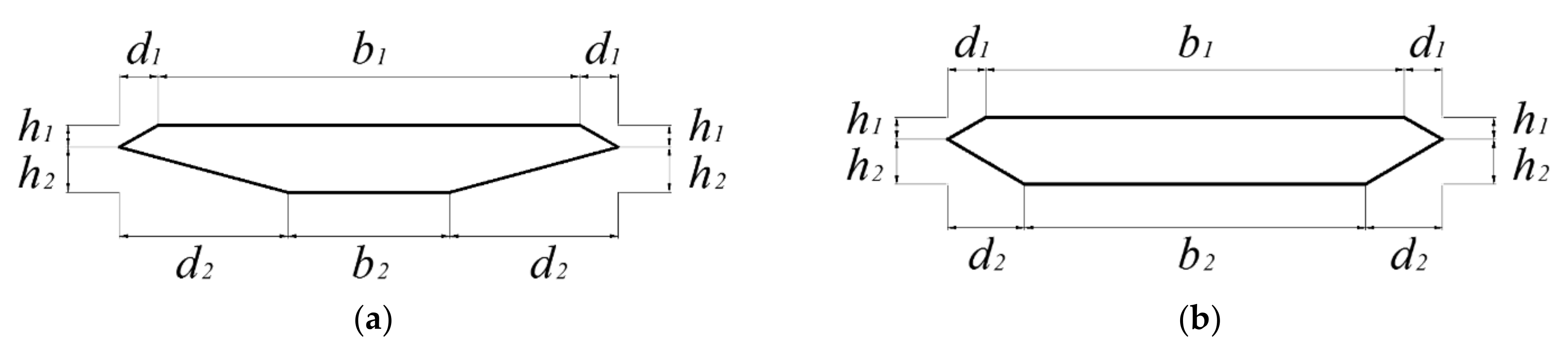
Figure 1. Cross section for Mod01 (a) and Mod02 (b) [3].
Infrastructures 06 00053 g001
Figure 2. Experimental model during pressure tests [3].
Infrastructures 06 00053 g002
Figure 3. Example of tunnel test velocity time history during test.
Infrastructures 06 00053 g003
Figure 4. Variability of the mean wind velocity (a) and air density (b) for all wind angles of attack.
Infrastructures 06 00053 g004
Figure 5. Variability of the mean wind velocity (a) and air density (b) for all wind angles of attack. In the legend Exp. Means the empirical CDF, Rayleigh means the Rayleigh CDF.
Infrastructures 06 00053 g005
Figure 6. Example of pressure coefficient time history for Mod01, angle of attack −10°.
Infrastructures 06 00053 g006
Figure 7. Standard deviation of the mean pressure coefficients non-dimensionalized on the wind velocity for Mod01 (a) and Mod02 (b); # means pressure tap number.
Infrastructures 06 00053 g007
Table 1. Geometrical dimensions of the test models [3].
h1h2d1b1d2b2
(mm)(mm)(mm)(mm)(mm)(mm)
Mod0113272125010096
Mod0213272125046204
Table 2. Mean and standard deviation of the wind velocity. Numbering from #1 to #4 means the four sets of wind velocity used to non-dimensionalize the pressure time history.
θ
(°)
U ¯
(m/s)
σ U
(m/s)
SetSet
#1#2#3#4#1#2#3#4
−108.3314.7621.0526.520.130.220.310.30
−88.4514.8621.2926.700.150.220.310.32
−68.4214.9821.3026.780.120.240.260.34
−48.5715.1221.5726.980.170.250.270.33
−38.6415.1421.5927.130.140.220.290.37
−28.5315.1121.5427.190.150.220.280.32
−18.5815.2321.7427.290.170.220.280.31
08.7915.2321.7727.440.160.210.280.34
18.7315.4021.8527.340.180.230.280.31
28.6515.3721.8827.480.140.210.290.33
38.8215.4621.9627.690.190.200.290.29
48.8715.4321.8627.560.150.210.220.26
68.7615.4822.0127.710.130.190.240.25
88.8515.5822.1827.880.140.190.220.22
108.9015.7622.3328.120.130.210.220.24
Table 3. The kinetic pressure estimated with the mean wind velocity. Numbering from #1 to #4 means the four sets of wind velocity used to non-dimensionalize the pressure time history.
θ
(°)
1 2 ρ U 2 ( Pa )
Set
#1#2#3#4
−1039.59124.32252.67399.68
−840.75126.07258.55405.75
−640.57128.39259.21408.86
−441.99130.75265.85414.79
−342.70131.13266.46419.88
−241.68130.81265.62422.19
−142.18132.93270.70425.55
044.63133.98273.48433.46
143.93136.69274.90429.29
243.01135.87275.20433.16
344.72137.42276.97439.09
445.13136.60273.96434.57
644.04137.58277.83438.91
844.88139.15281.81444.35
1045.37142.35285.57451.87
Table 4. Standard deviation of subintervals mean wind velocity. Numbering from #1 to #4 means the four sets of wind velocity used to non-dimensionalize the pressure time history.
θ
(°)
σ U ¯ t i ( m / s )
Set
#1#2#3#4
−100.100.170.260.22
−80.120.180.270.26
−60.080.200.200.29
−40.150.220.220.27
−30.110.180.240.32
−20.110.170.220.26
−10.140.170.230.25
00.130.170.230.28
10.150.190.220.24
20.100.170.240.27
30.170.150.240.22
40.130.160.150.19
60.090.140.180.17
80.100.130.150.14
100.100.160.160.16
Table 5. Gaussianity according to [37].
θ
(°)
Set
#1#2#1#2
−100010
−80010
−60101
−41101
−30001
−20000
−10100
00011
11000
20000
31110
41000
60000
80001
100010
Publisher’s Note: MDPI stays neutral with regard to jurisdictional claims in published maps and institutional affiliations.

