Article

Predicting Oil Production Sites for Planning Road Infrastructure: Trip Generation Using SIR Epidemic Model

1
Management Department, New Jersey City University, Jersey City, NJ 07311, USA
2
Mathematics Department, New Jersey City University, Jersey City, NJ 07305, USA
*
Author to whom correspondence should be addressed.
Infrastructures 2021, 6(2), 15; https://doi.org/10.3390/infrastructures6020015
Submission received: 16 December 2020 / Revised: 9 January 2021 / Accepted: 17 January 2021 / Published: 21 January 2021

Abstract

:
Drilling activity produces a significant amount of road traffic through unpaved and paved local roads. Because oil production is an important contributor to the local economy in the state of North Dakota, the state and local transportation agencies make efforts to support local energy logistics through the expansion and good repair and maintenance of transportation infrastructure. As part of this effort, it is important to build new roads and bridges, maintain existing road pavement and non-marked road surface conditions, and improve bridge and other transportation infrastructure. Therefore, the purpose of this study is to review previous oil location prediction models and propose a novel geospatial model to predict drilling locations which have a significant impact on local roads, to verify and provide a better prediction model. Then, this study proposes a SIR (susceptible–infected–recovered) epidemic model to predict oil drilling locations which are traffic generators. The simulation has been done on the historical data from 1980 to 2015. The study found that the best fit parameters of β (contact rate) and μ (recovery rate) were estimated by using a dataset of historical oil wells. The study found that the SIR epidemic model can be applied to predict the locations of oil wells. The proposed model can be used to predict other drilling locations and can assist with traffic, road conditions, and other related issues, which is a much needed predictive model that is key in transportation planning and pavement design and maintenance.

Graphical Abstract

1. Introduction

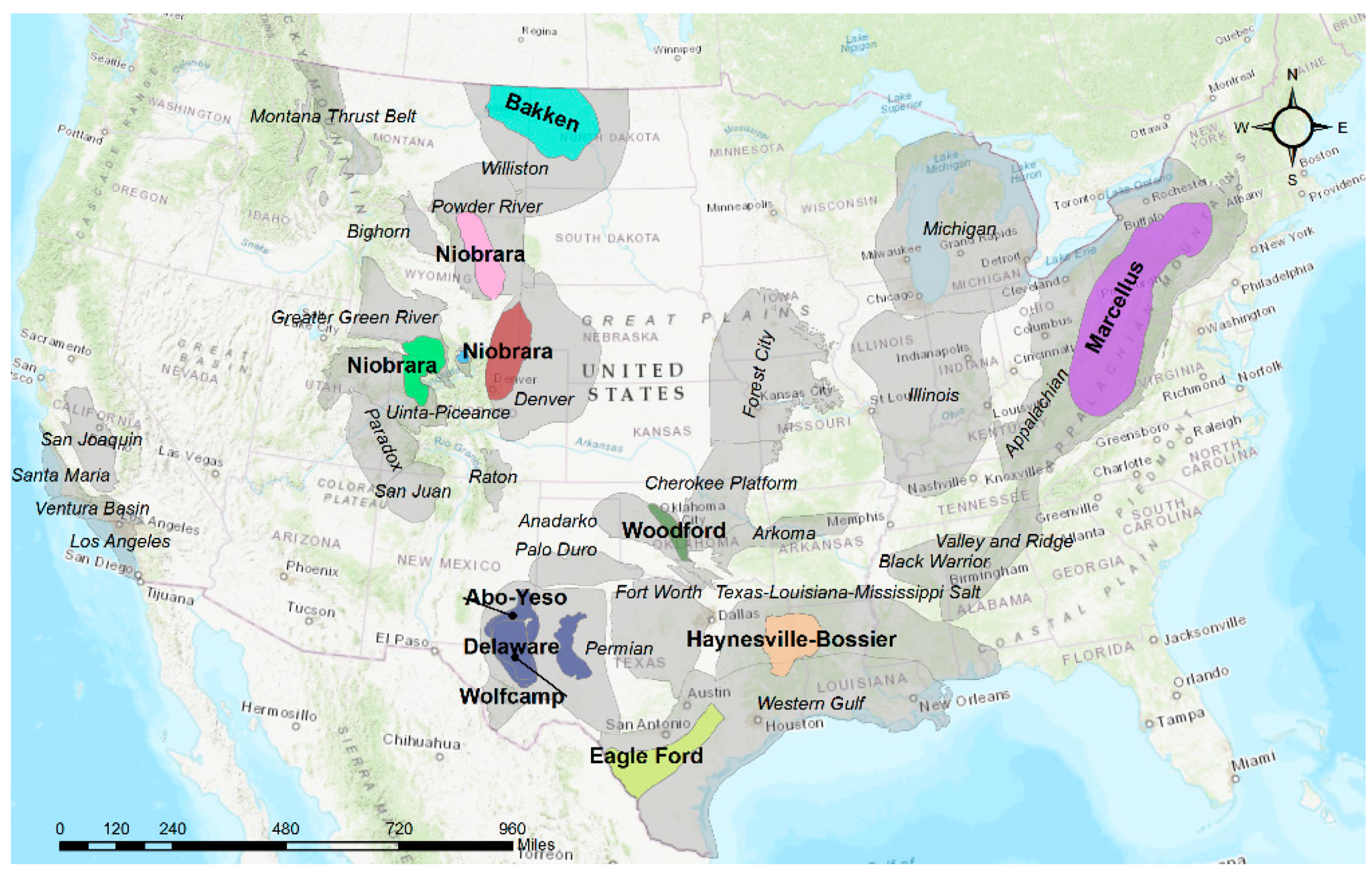
Due to the increase in oil prices and rapid advancements in drilling technologies known as horizontal drilling and hydraulic fracturing (i.e., fracking), the number of oil wells has increased since the mid-2000s [1,2,3]. As shown in Figure 1, the most productive oil and natural gas production regions are Bakken, Niobrara, Permian, Eagle Ford, Haynesville, Utica, and Marcellus shale formations across the United States [4]. The technologies require a significant amount of water, fracking sand, and other additives [1]. The median duration of drilling time for horizontal drilling has also significantly increased, from approximately one month in 1977 up to three to four months in 2013, from permit approval to well completion, in Texas [1].
Drilling activity occurs prior to the process of oil production. Drilling activity produces a significant amount of road traffic through unpaved and paved local roads, thereby causing poor pavement conditions [1]. The total number of truck movements is estimated to be 2300 truck trips to construct one well, which is a sum of 1150 loaded truck movements for inbound logistics and 1150 empty truck movements for backhaul [7].
Oil production activity is a source of extracted outbound traffic of crude oil and salt water. Production is estimated to be determined by the market price, location, and oil reserves of oil wells. The produced crude oil is transported by a truck to a storage tank, train terminal, or pipeline storage and by a pipeline to a rail terminal and/or pipeline storage tank. At this point, the amount of traffic caused by the truck trips affects the life and condition of the roads [8].
Because oil production is an important contributor to the local economy, the oil producing state and local transportation agencies (i.e., counties and cities) make efforts to support local energy logistics through the expansion and good repair and maintenance of transportation infrastructure [1]. It is crucial to keep the community and logistics operators safe [9]. As part of this effort, it is important to build new roads and bridges, maintain existing road pavement and non-marked road surface conditions, and improve bridges and other transportation infrastructure by projecting likely levels of activity [10]. To create a new road and connect the feeder roads to a local road network that already exists, transportation planners and engineers need information about the new drilling locations.
Thus, if the infrastructure planner and pavement designer do not take the heavy traffic volume into account, the service life of the pavement might be shorter than the design life of the pavement. This increases user costs and the maintenance costs of the roads in a reactive mode [1] as well as road accidents and crashes [9].
In the early interstate program, pavement design principles and practices adopted a 20-year period of performance as the standard design life for federal-aid projects [11]. While some states aimed at maintaining the performance of pavements for over 20 years, the state of North Dakota adopted the 20-year standard for pavement design and future traffic growth using ESAL (an equivalent number of standard or equivalent loads). It is relatively simple to determine the standard ESAL for only agricultural traffic in the west of North Dakota, but it is complicated to estimate due to a number of types of axle loads and vehicle configurations [12]. The most common equation is the 18,000 lb (80kN) equivalent single axle load in the U.S. [13]. By accurately estimating ESAL, the planner can design a pavement life which is close to the service life of the pavement.
Transportation planning relies heavily upon transportation demand modeling for long-term pavement design and budget planning. In North Dakota (ND), the Department of Transportation (NDDOT), in collaboration with the Upper Great Plains Transportation Institute (UGPTI), forecast traffic volume on roads [3]. ND predicts traffic on the roads caused by oil production and oil development based on a four-step travel demand model: trip generation, trip distribution, mode choice, and trip assignment [7]. The first step of modeling is predicting trips derived from economic activities, called trip generation. In the second step, the technical reports utilize a variety of modeling techniques including optimization, gravity, and regression models [7]. Regardless of the techniques used in the second step, all models rely upon predicted potential drilling locations as a source of trips. This is a complicated task since many factors such as distance from water, travel distances, and reserves are involved, and contracts between private landowners and oil developers are confidential [12]; therefore, this creates challenges for transportation modelers. The relationship and dynamics between these factors are uncertain [2,12]. Previous studies have attempted to use several different methods including maximum likelihood [3] and logit regression [7,14] to predict potential drilling locations in a given time at different levels of spatial granularity. As these studies expand, this study developed a combined epidemic model with geospatial analysis to identify the most likely future drilling sites and oil wells.
Therefore, the purpose of this study is to review previous oil location prediction models and propose a novel geospatial model to predict drilling locations which have a significant impact on local roads, to verify and provide a better prediction model. Then, this study proposes a SIR (susceptible–infected–recovered) epidemic model to predict oil drilling locations which are traffic generators. This study will benefit transportation planners and modelers by identifying approximate drilling sites of trip sources, which will enable better planning of management and financial budgeting processes in areas associated with oil production.

2. Literature Review

2.1. Space Choice Models

Space choice modeling was compared by Hunt, Boots, and Kanaroglou [15]. The study provided general choice models and then attempted to add a spatial component in the choice models, resulting in the spatial choice model. They introduced other choice models including the generalized extreme value model, the open-form choice model, and the choice set model. The study proposed that these models are evolved by taking into account the spatial factor and random utility function. Likewise, Bhat and Sener [16] used a spatial logit model to accommodate spatial correlation among sample units. They proposed a copula-based, closed-form, binary logit choice model. Their method highlights the power of closed-form techniques for accommodating spatial effects.
Zhu and Timmermans [17] extended the heuristic rules, conjunctive, disjunctive, and lexicographic rule, and introduce heterogeneity. Alamá-Sabater, Artal-Tur, and Navarro-Azorín [18] introduced the neighborhood effect in the spatial conditional logit framework. They investigated the drivers of the location choices of industrial firms in cases of inter-territorial spillovers. They confirmed the influence of the spatial factors on the decision analysis with other major factors. They developed their model based on the standard random utility maximization (RUM) framework.
For these patterns and spatial choice models, geographic information systems (GIS) are widely used to predict the random movements of people, animals, diseases, and other biological organisms. These spatial analyses incorporate multiple data sources such as locations, historical pathways, and boundaries [19]. Along with spatial pattern analysis, pattern recognition analysis is commonly used to recognize patterns referred to as sets of statistical techniques [20]. These techniques have been applied to pandemic, crime analysis, and biology studies. To estimate randomly distributed locations, several spatial pattern analyses were introduced in criminal analysis, disease, and epidemic models to handle dynamic movement under uncertainty.

2.2. Epidemic Models

Volz and Meyers [21] introduced a new model, called neighbor exchange (NE). This model is dynamically added to the static access network model. The model assumes that each individual will be in contact with a specific number of individuals who are capable of transmitting diseases at any given time. Each contact is temporary and lasts for a variable amount of time before it ends. This model captures the populations’ dynamic characteristics of the epidemic propagation, thus capturing the susceptible–infected–recovered (SIR) dynamics in a population [22,23]. The SIR model is used in epidemiology to compute the amount of susceptible, infected, and recovered people in a population. It is also used to explain the change in the number of people needing medical attention during an epidemic [24,25,26]. It is important to note that this model does not work with all diseases. For the SIR model to be appropriate, once a person has recovered from the disease, they would receive lifelong immunity. The SIR model is also not appropriate if a person is infected but is not infectious [25,27,28]. Bertuzzo et al. [29] conducted research on the propagation of cholera through the hydrological network connections. They tested different lattice models as networks to calculate the front speed of an epidemic. They suggest that their approach presents a better solution for heterogeneous networks. Danon et al. [30] used a degree of distribution to present a risk assessment model of infection in a social network. They used surveys to generate better results from their model. They provided survey results and implications about different models, which use different assumptions to model disease propagation in a social network.

2.3. Spatial Prediction of Drilling Locations

Since 2010, the Upper Great Plains Transportation has conducted research on North Dakota’s road investment to support oil and gas production and distribution. To estimate the impact of inbound logistics for drilling activities on the local roads, studies projected future drilling sites. The 2010 study [31] assumed that the first drilling started at the last year of the lease to secure the lease. In the following years during Phase II, 3–5 wells were randomly added across public leases as well as private leases. The drilling activity was assumed to happen in sections. The 2012 [3] study used the base unit of the spacing unit, one mile by two mile geographic area with 1280 acres. The number of new wells was constrained by the projected number of wells by the ND Oil and Gas Division. The study used a probabilistic method, namely a maximum likelihood algorithm, including spatial and non-spatial factors with a threshold of yearly projected wells. Highly likely new wells were selected for a year, and all other wells were listed in the following years to be selected. In the 2014 study [7], the fishnet procedure in ArcMap was added onto the public spacing units to place future oil wells. The study assumed that 8–12 wells would be drilled, and each spacing unit would have two oil pads. While the previous study used the number of new wells across the state as a threshold, this study started to combine the county-level new wells yearly. Based on the existing wells, the hot-spot analysis showing the concentration of oil activities was used to locate future oil wells. The prediction model was not intended to provide each well’s location. In the 2016 study [32], there were several significant changes in factors. The study assumed that each spacing unit would accommodate 20–24 wells due to advances in technology and the estimate of the reserves. The productivity of a rig increases by 10–12 wells per year. To reflect market and production uncertainty, the study applied three scenarios based upon 30, 60, and 90 active rigs in the region. The number of new wells is constrained by either statewide forecast or county-level forecast which reaches first. In the 2020 study [33], each spacing unit accommodates 8–20 wells for its life. By clustering the existing wells and adding new wells, the hot-spot analysis provided new potential sites for new wells. As used in the previous study, statewide number of wells and county-level projected wells are used as constraints for placing wells per year [34].
In 2010, Johnson et al. [35] projected new natural gas and wind energy development sites in Wayne County in Pennsylvania, located in the Marcellus shale region, using low, medium, and high development scenarios. The study used the maximum entropy model to estimate the surface probability of gas wells and wind turbines using existing locations. The maximum entropy (also known as Maxent) was run by a machine-based learning approach to find relationships between existing and permitted wells and a variety of variables adopted by the oil companies. The variables include shale depth, thickness and thermal maturity, and the probability of an area to potentially support future gas well development. The study did not include the precise locations of energy company leases. Thus, the study projected the location of gas wells with the overall geographic patterns.
In 2011, Lee et al. [36] evaluated the impact of developing high-volume hydraulic fracturing (HVHF) for natural gas on the rural areas and forest in Tioga County in NY, which is located in the Marcellus Shale formation. The study conducted spatial analysis by modeling the number of well pads expected to be constructed and the number of spacing units in the county. The study was conducted based on an average spacing unit of 160 acres, and 90% of wells will be constructed by horizontal drilling. It also assumed that each well pad would allow up to six horizontal wells. The initial plan of the number of wells was based on the estimates of the Economic Assessment Report published by the New York Department of Environmental Conservation (NYDEC). The report established three scenarios of low, medium, and high development since the level of development was not known. In practice, 6–10 wells per oil pad are likely to be drilled, but the number of wells is not required to drill. It is entirely dependent on the profit, production, and operation costs. By permitting multiple wells per oil pad, this will significantly minimize the impact of construction and production on the roads and natural resources [37]. The model used a build-out analysis for the next 30 years until the technically recoverable reserves are exhausted.
In 2012, Alan [12] used the SIR epidemic model to predict oil wells to estimate the traffic volume on local roads due to oil activities in North Dakota and Montana. The model projected the number of oil wells in a time horizon per township. A township includes around 18 multiple spacing units and each 1280-acre spacing unit is allowed to drill six wells. In practice, the Bakken formation drills 5–7 wells per spacing unit; however, he used the average number of oil wells being drilled in a spacing unit by the horizontal drilling technique. The study also constrained the number of drilling wells based on the county’s production plan by Phase I and Phase II. At least one well is expected to be drilled in Phase I to secure leases, while Phase II is a filling-in drilling stage with up to six wells. The SIR model reflects a spatial clustering approach. The model is also based on the information available from the ND Oil and Gas Division. The model used the number of new wells per year to measure for validation.
In 2014, Lee et al. [14] projected oil well locations using the spatiotemporal maximum likelihood estimation approach. The model uses several factors including the US Geological Survey’s oil assessment information, proximity to the pipeline loading sites, fresh water depots and the closest well, area density, and well age. The study predicted the new oil wells in seven oil zones across 17 oil counties in North Dakota. The model found that zone density and number of oil wells within 15 miles were the most significant factors. It proved that the cluster of oil wells is a crucial factor since the clustering is productive and cost-effective, connecting pipelines and close to the crude-by-rail terminals.
In 2016, Hanson, Habicht, and Faeth [2] investigated the impact of natural gas development using hydraulic fracturing in Pennsylvania, located in Marcella shale region. The study developed a geospatial analysis to locate the most likely future well locations. This study used the existing well locations as a base layer describing the characteristics of shale formation and infrastructure. To estimate the likelihood, the study combined the probability surface with the most recent estimate of total recoverable reserves and average production rate for each well. The model also utilized a build-out approach by setting the ultimate amount of gas to extract based on the information about the gas reserves in the region and the technology available to recover the gas. Their build-out analysis estimated 47,600 additional wells and over 5950 well pads for the next 30 years. Horizontal drilling enabled drilling of multiple wells per well pad, thereby increasing the efficiency and speed of gas production [2]. The study estimated the most likely well pad locations first and then distributed the number of projected wells across the well pads using the combined geospatial analysis and maximum entropy model. The estimation used historical well locations and geological and environmental data layers. The study assumed that all wells were drilled by horizontal drilling techniques and up to eight wells would be allowed per oil pad in a fixed spacing over the 30-year time horizon.
After reviewing the previous studies, they indicate that drilling locations can be estimated by using a SIR epidemic model. The required spatial information of existing well locations and oil pads can be collected, and the outputs of oil wells projected by the SIR model can be visualized by using geographic information systems (GIS). To our knowledge, based on an intensive literature review, we found that there is a need for a novel spatial model for predicting horizontal drilling locations over a long-term period to support transportation planning and pavement design.

3. Datasets and Methods

3.1. Data Description

An oil spacing unit represents the public land lease for drilling and producing oil, being used as traffic analysis zones (TAZ), available from the North Dakota Oil and Gas Division. The division provides all oil activity-related GIS files through ArcIMS Viewer [38]. Historical oil wells and existing rig locations are available from the information server. The number of drilling rigs is an important indicator of future oil development and production [33]. The number of wells being drilled is closely correlated with market condition (Figure 2a) and the number of rigs and their productivity (Figure 2b). The downloaded GIS shapefiles were imported into Python for further analysis based on the primary key of API (American Petroleum Institute) well numbers, which are unique identifiers for wells. The output of the SIR model was reimported into ArcGIS for the visualization process.
The previous active oil wells can be tracked by spud year in the given oil wells from the North Dakota Department of Mineral Resources [38]. The years 2005 to 2018 were considered in the historical period to estimate the oil production and historical rig locations in time series. Thus, the prediction model does not account for the oil wells located outside of the spacing units in 17 counties in ND. This study visually compares the forecasting data from the North Dakota Department of Labor for the number of oil wells in the next 50 years through oil zones [34].

3.2. Assumptions

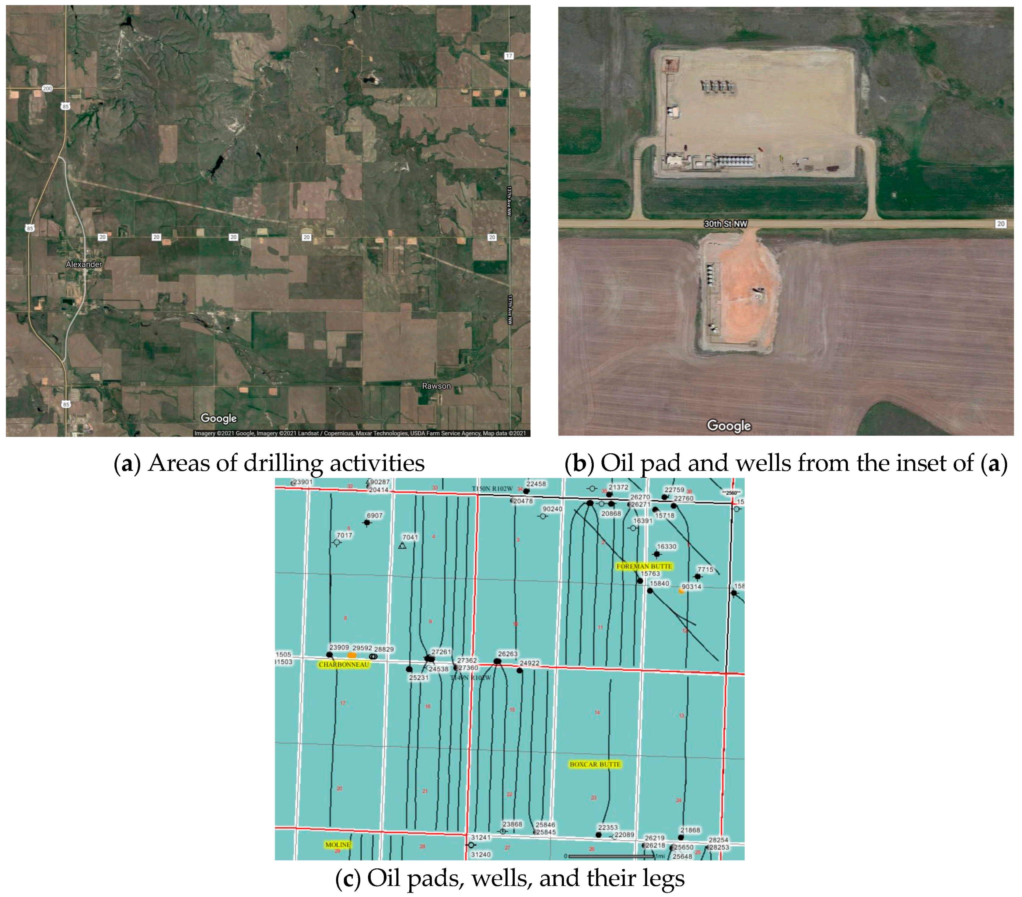
It is expected to be a slow response to the demand and inflexible when new wells are constructed from the distant points from the existing gathering pipelines and oil collection points, and from the existing road infrastructure (see Figure 3a). Therefore, per rational behavior, the study expects that the oil companies are highly likely to determine new oil wells which are close to the infrastructure to transport large quantities and are in the midst of oil clusters [40].
Phase I involves the drilling of a single well at the end of a lease period to secure the license. Phase II will add oil wells to complete the spacing unit development. The spacing unit used in this study is assumed to be 1280 acres at 1 mile and 2 miles of existing public lease units. The analysis zones used in the study have survey townships, which belong to a county, and the county has an annual planned number of wells. Therefore, the sum of the number of existing active wells and new wells cannot exceed the planned number of oil wells. In other words, the projected wells are added to the existing wells from the previous years. It is assumed that the above spacing units may have multiple oil pads, but up to new six wells are assumed to be drilled per oil pad (Figure 3c). The rigs placed in the area are most likely to be 60, and the productivity of a rig is assumed to be up to 24 wells per year for the Upper Great Plains Transportation Institute [33]. However, in consideration of drill site preparation and rig movement time from an oil pad to the other pad, the model assumes that, at most, one well is drilled in a spacing unit per year.

3.3. Model Development: SIR

In this paper, the susceptible–infected–recovered (SIR) model is used as a method of future oil development. The SIR model was developed to model the spread of epidemics, thereby classifying portions of a population as susceptible, infected, or recovered at different time periods [23,26,28,41]. The total population is equal to S + I + R. A person may move from S to I and I to R, but not from R to I or I to S. For the purposes of this study, the susceptible group (S) represents townships in which oil development has not yet occurred or is in the early stages of development. The infected group (I) represents townships that have completed Phase I drilling. Phase I drilling refers to drilling at least one well per spacing unit to secure leases. The recovered group represents spacing units that have completed the Phase II “filling-in” stage.
The area of the typical spacing unit is 1280 acres or 2 square miles, which is equivalent to an individual. The spacing units will be one of the categories of susceptible (S), infected (I), or recovered (R), which are the set of dependent variables.
The dependent variable is the function of time (t). The number of susceptible (St + 1) is determined by the number of already susceptible (St), the number of spacing units already infected (It), and the amount of contact (β) between susceptible units (St) and infected units (It) (Equation (1)). The number of infected (It) is the number of infected individuals (i.e., spacing units) (Equation (2)). It represents the infected fraction of the population (i.e., total number of spacing units). It assumes that each infected individual has come into contact with a fixed number β of contacts per day, which is a fraction of the susceptible. Thus, βSt is the newly infected individuals per day. R is the number of recovered individuals (spacing units) (Equation (3)). Thus, Rt is the recovered fraction of the population (total spacing units).
It is determined by the number of already infected (It), the amount of contact between susceptible (St) and infected (It). It assumes that a fixed fraction of μ of the infected spacing units will be recovered during any given year. In other words, an infected spacing unit becomes dry, resulting in no activity for producing oil. No trips will be generated from the dry spacing unit. The model is given by [24,26,28,41]:
S t   +   1 = S t β S t I t ,
I t + 1 = I t + β S t I t μ I t
R t   +   1 = R t + μ I t ,
where the parameter β is known as “contact rate” and μ is known as “recovery rate.” In the oil forecasting usage, β represents the spread of Phase I development, which is historically based upon geographic location and proximity to existing wells and μ represents the time period corresponding with Phase II or “fill-in” drilling. The bilinear incidence term βStIt for the number of new infected individuals per unit time corresponds to homogeneous mixing of the infected and susceptible classes.
For the numerical simulations, we considered the following assumptions:
  • Susceptible spacing units: If the number of recovered wells in one spacing unit is less than six or equal to six.
  • Infected spacing units: At least one well is drilled but less than or equal to five in one spacing unit.
  • Recovered spacing units: Six wells or more were drilled in one spacing unit, exploration is complete.
The number of available spacing units at the beginning of the year 2015 was 33,726 where the number of susceptible spacing units is 32,679, the number of infected spacing units is 259, and the number of recovered spacing units is 788.
Using the methodology outlined in Tome and Ziff [42], a stochastic lattice model with asynchronous dynamics with corresponding distribution algorithm has been developed. Each site can be occupied by only one of the states of S, I, or R. According to Tome and Ziff [42], at each time step, a site is randomly chosen, and the following rules are applied:
  • If the chosen site is in state S or R, it remains unchanged.
  • If the chosen site is in state I then
    • with probability c, where the chosen site becomes R and c = μ / ( μ + β )
    • with the complementary probability (b = 1 − c), a neighboring site is chosen at random. If this is in state S, it becomes I; otherwise, it remains unchanged.
Tome and Ziff [42] simulated the SIR model by using a dynamic Monte Carlo method. The procedure begins with the random selection of an infected (I) site from the available list of infected sites. Next, a random number x in (0, 1) is generated. If xc, then infected (I) becomes recovered (R). If xc, one of the four nearest neighbors of the infected (I) site is randomly selected. If the neighbor is susceptible (S), then it is now infected (I), and added to the list of infected sites. This procedure is repeated as long as any infected sites remain.

3.4. Model Calibration and Validation

The best fit parameters of β (contact rate) and μ (recovery rate) were estimated by using a dataset of historical oil wells of the period of 2005–2015. Root mean squared errors (RMSE) were calculated for estimating the best calibration parameters of the model. The simulation was conducted on historical data from 1980 to 2015, for various values of β and μ. To find the best pair of (β, μ), the model was validated over the years 2016–2018. From Table 1, it is found that for β = 0.000021 and μ = 0.20, RMSE is minimum. It is also found that the SIR model is very sensitive to the values of β and μ.
For model validation, Table 2 depicts the comparison of the number of actual oil wells per spacing unit and the predicted number of infected sites with β = 0.000021 and μ = 0.20. Furthermore, it is found that, on average, 80% actual sites match with the prediction. On the basis of this information, we ran the simulation associated with the system (t) for the next 50 years starting from 2015. It is observed from the graphs that the number of infected sites obtains the maximum value during the year 2035.

4. Results and Discussion

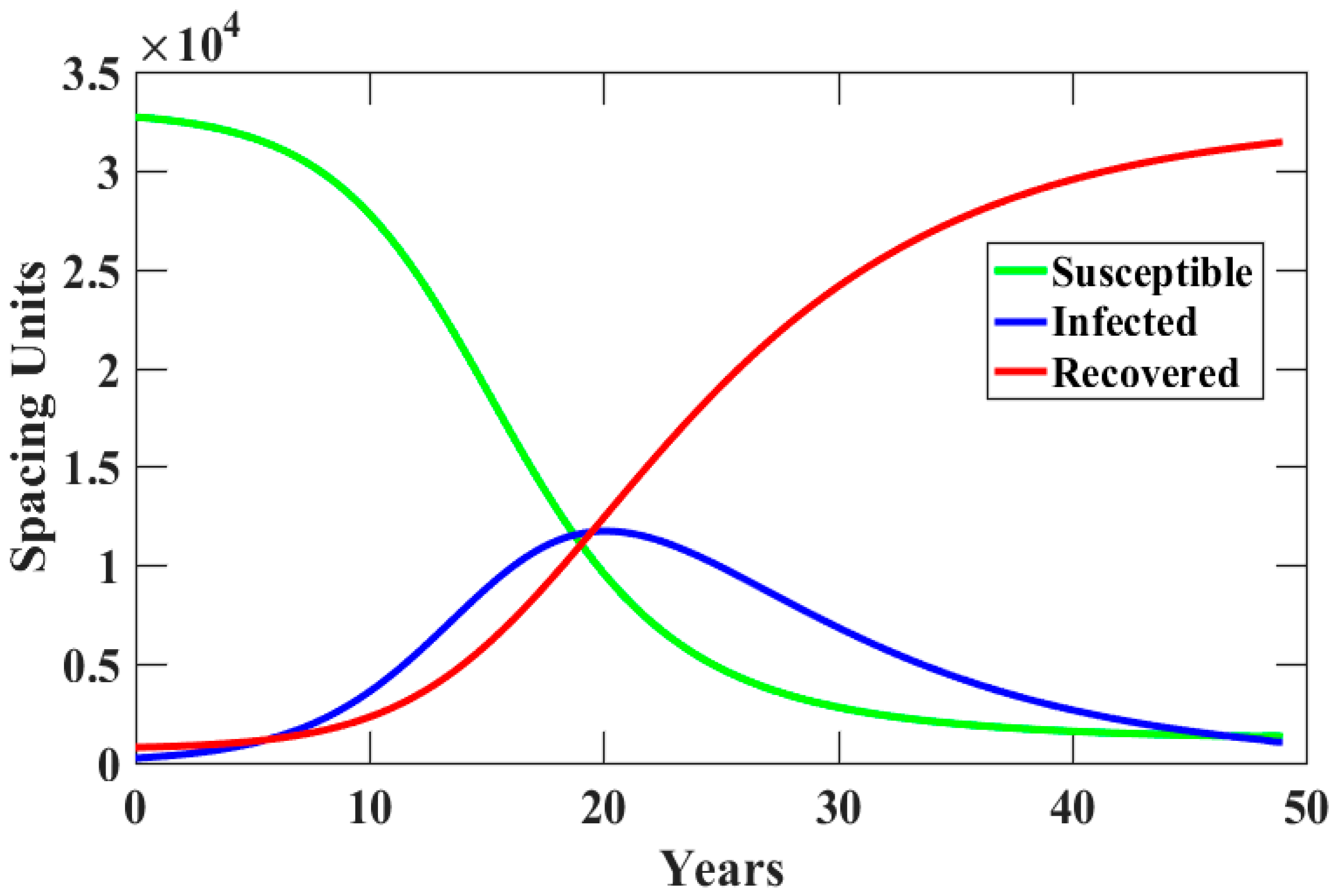
In the graph (Figure 4), the x-axis shows the flow of time in years from the beginning of the new transportation planning year. The y-axis represents the number of year-by-year spacing units included in the three categories of susceptible, infected, and recovered. The model begins with 33,723 spacing units and 259 initial infected (i.e., being drilled) spacing units.
The green line means the number of susceptible zones for a year that have not yet been drilled but it is an area where drilling can be carried out at any time. The number of zones gradually decreases after 10 years, and by the 30th year, the number decreases rapidly, and then the number slows down over time as the number of mining areas decreases significantly.
The blue line refers to the total number of infected zones for a year that have already been mined or have been producing for several years. This line is basically an epi-curve that directly affects oil production. The number of zones gradually increases, then peaks in the 20th year, with the number of drilling areas reaching around 12,000, and decreases gently over time. The number of production areas is reduced by the 50th year, when nearly 30,000 zones hold wells. Each zone can develop up to six wells even if a zone has a few oil wells, so the actual number of oil wells is larger than the number of infected zones where this drilling is made. The 18th year of intersection of susceptible (green) and infected (blue) will be the first year when the actual zone with oil wells exceeds the number of areas that are likely to be developed. The right tail of the blue line means recovery rate, with the first 788 zones no longer available for drilling, and the annual number of areas with no more possibilities for drilling is seen after eight years.
The red line indicates the number of areas where oil well drilling no longer takes place, and as the number continues to increase until 40 years later, continuous drilling is expected. From the 18th year, when the red and green lines intersect, the number of areas where the drilling is completed will exceed the number of areas where the drilling proceeds. When applied to actual life forms, the total number of recovery patients may be less than the number of recovered patients due to the death toll, but in our model, the number of areas where drilling has been completed will be the same as those where drilling is to be conducted, unless the areas where drilling is given up are considered. However, the graph above shows no additional recovery rate (i.e., drilling completion rate) because it was modeled for up to 50 years.
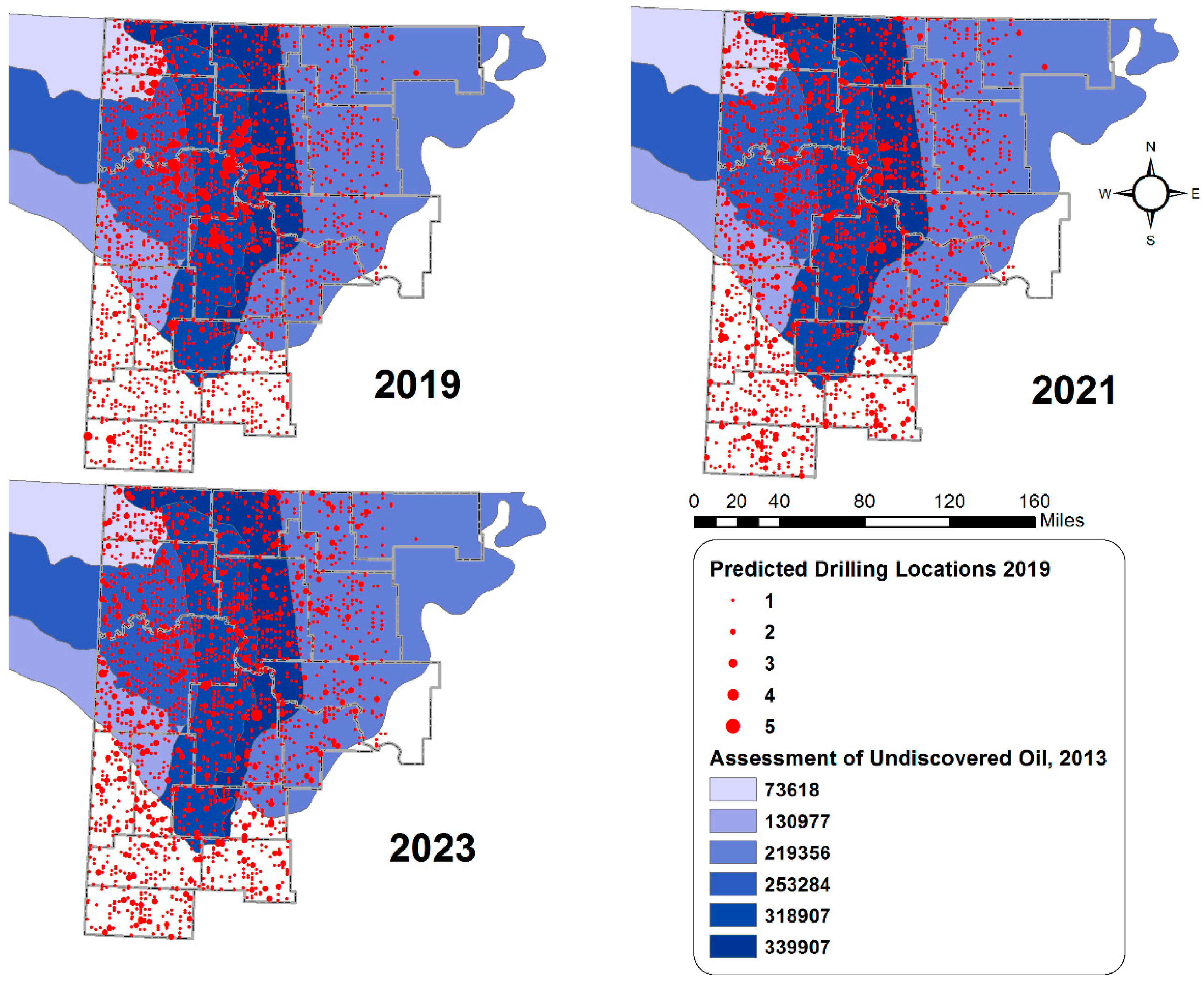
Figure 5 visualizes the distribution of drilling locations which are in the beginning state of infection in the years of 2019 (I2019), 2021 (I2021), and 2023 (I2023). The majority of drilling activities are over the conventional and continuous oil assessment areas near the dark blues in the middle of the Bakken Formation. In the figures, the predicted number of barrels of undiscovered oil in 2013 is shown in varying color intensity. While drilling activities are concentrated in the assessment areas in the year of 2019, the activities are distributed across the region.
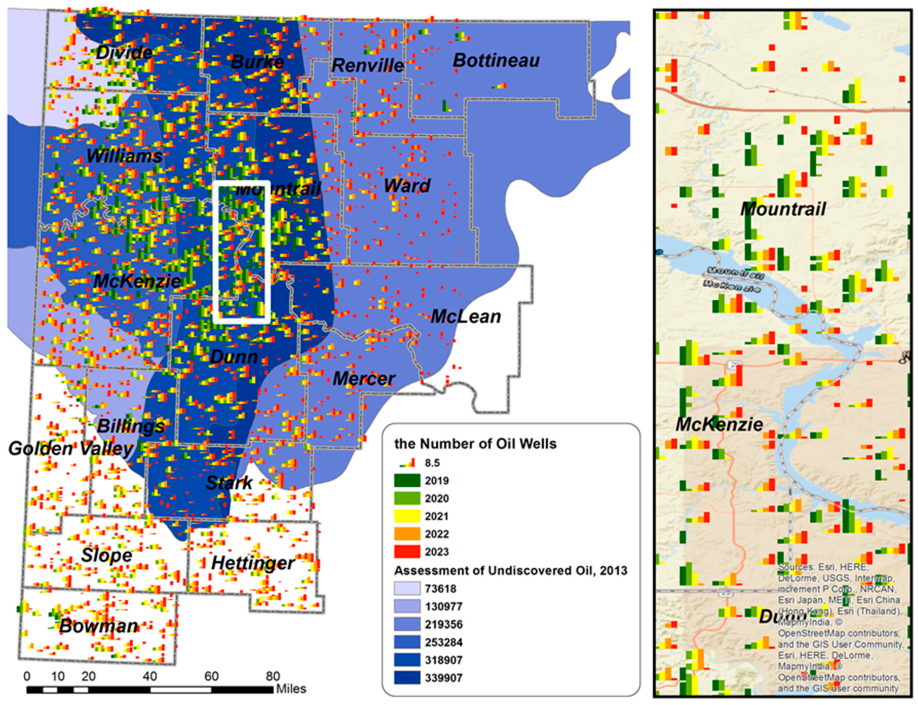
Figure 6 shows the oil wells being pumped for the next five years from 2019 by spacing unit in a bar graph. As of 2019, production was carried out in areas with large reserves and was gradually spreading to nearby areas. In particular, it is active in production in the western 120-mile zone. Through this, it is deemed that within two to three years, roads nearby the production site will need to be paved or improved, and three years later, active production areas will have to establish new construction or special road treatment and maintenance measures.
Hanson et al. [2] recognized that its model outcomes would be changed significantly by changing estimates. Changing the total number of planned wells is relatively simpler than projecting well locations. The changes will have a huge impact on the traffic volume on local roads and pavement conditions. The model will be changed and updated in response to better information about production plan, geological data, technology advance, and market conditions [2]. Thus, to mitigate the consequences of uncertainty of the parameters, Upper Great Plains Transportation and ND Department of Transportation will update the studies every two years [36].

5. Conclusions

This study investigated previous research and used a novel geospatial model to predict drilling locations using the SIR epidemic model, to verify and provide a better prediction model. Thus, this study proposed a SIR (susceptible–infected–recovered) epidemic model to predict oil drilling locations which are traffic generators. The proposed model not only provides better predictive results, but it also aims to enable organizations to adopt the model more easily. Therefore, this study benefits transportation planners and modelers by identifying approximate drilling sites of trip sources, which will enable better planning of management and financial budgeting processes in areas in which oil production takes place.
After studying and analyzing this information, we ran the simulation associated with the system (i) for the next 50 years starting from 2015. It is observed from the graphs that the number of infected sites reaches the maximum value during the year 2035. When the results are applied to actual life forms, the total number of recovery patients may be less than the number of recovered patients due to the death toll, but in our model, the number of areas where drilling has been completed will be the same as those where drilling is to be conducted, unless the areas where drilling is given up are considered. However, the data show no additional recovery rate (i.e., drilling completion rate) because it was modeled for up to 50 years.
The study found that as of 2019, production was carried out in areas with large reserves and was gradually spreading to nearby areas. In particular, it is active in production in the western 120-mile zone. Through this, it is deemed that within two to three years, roads nearby the production site will need to be paved or improved, and three years later, active production areas will have to establish new construction or special road treatment and maintenance measures.
As a result of this study, the proposed model can be used to predict other drilling locations and can assist with traffic demand management, road conditions, and other infrastructure-related issues, which is a much needed predictive model that is key in planning and fiscal management. Although the proposed model in this study will predict the trips occurring with established parameters such as drilling wells and the production of oil in a certain pattern, the parameters of the model need to be properly modified to account for economic disruption or emergencies such as COVID-19 and the plunge of world gas price. Political decisions also affect mining and production activities. Therefore, it is recommended that the long-term predictive model presented here be updated periodically and long-range estimates carefully interpreted.

Author Contributions

Conceptualization, E.L.; Methodology, E.L. and D.C.; Software, E.L. and D.C.; Validation, D.C.; Formal Analysis, E.L., D.C., M.M.; Investigation, E.L., D.C., and M.M.; Data Curation, E.L. and D.C.; Writing—Original Draft Preparation, E.L. and D.C.; Writing—Review and Editing, M.M.; Visualization, E.L. and D.C.; Supervision, Project Administration, E.L. All authors have read and agreed to the published version of the manuscript.

Funding

This research received no external funding.

Institutional Review Board Statement

Not applicable.

Informed Consent Statement

Not applicable.

Data Availability Statement

Publicly available datasets were analyzed in this study. This data can be found here: https://www.dmr.nd.gov/OaGIMS/viewer.htm.

Acknowledgments

The author would like to thank editors and reviewers for their invaluable comments.

Conflicts of Interest

The authors declare no conflict of interest.

References

  1. Quiroga, C.; Tsapakis, I.; Kraus, E.; Le, J.; Wimsatt, A. Oil and Gas Energy Developments and Changes in Pavement Conditions in Texas; Texas A&M Transportation Institute: College Station, TX, USA, 2015; Available online: https://static.tti.tamu.edu/tti.tamu.edu/documents/PRC-15-35-F.pdf (accessed on 5 January 2021).
  2. Hanson, L.; Habicht, S.; Faeth, P. Potential Environmental Impacts of Full-Development of the Marcellus Shale in Pennsylvania; CNA: Arlington, VA, USA, 2016; Available online: https://www.delawareriverkeeper.org/sites/default/files/MarcellusPA_FullReport.pdf (accessed on 5 January 2021).
  3. Upper Great Plains Transportation Institute. An Assessment of County and Local Road Infrastructure Needs in North Dakota; North Dakota State University: Fargo, ND, USA, 2012; Available online: https://www.ugpti.org/resources/reports/details.php?id=903 (accessed on 5 January 2021).
  4. Energy Information Administration. Petroleum and Other Liquids. 14 December 2020. Available online: https://www.eia.gov/petroleum/drilling (accessed on 6 January 2021).
  5. U.S. Geological Survey. Assessment of Undiscovered Oil and Gas Resources of the Williston Basin Province of North Dakota, Montana, and South Dakota, 2008; USGS Central Energy Team: Lakewood, CO, USA, 2008. Available online: http://pubs.usgs.gov/fs/2008/3092/pdf/FS08-3092_508.pdf (accessed on 5 January 2021).
  6. U.S. Energy Information Administration. Maps: Oil and Gas Exploration, Resources, and Production. U.S. Department of Energy. Available online: https://www.eia.gov/maps/maps.html (accessed on 6 January 2021).
  7. Upper Great Plains Transportation Institute. Infrastructure Needs: North Dakota’s County, Township and Tribal Roads and Bridges: 2015–2034; North Dakota State University: Fargo, ND, USA, 2014; Available online: https://www.ugpti.org/resources/reports/downloads/2014-07-infrastructure-needs.pdf (accessed on 6 January 2021).
  8. Dybing, A.; Lee, E.; DeHaan, C.; Dharmadhikari, N. Impacts to Montana State Highways Due to Bakken Oil Development; Montana Department of Transportation: Helena, MT, USA, 2013. Available online: https://www.mdt.mt.gov/other/webdata/external/research/docs/research_proj/oil_boom/final_report.pdf (accessed on 6 December 2020).
  9. Quiroga, C.; Tsapakis, I. Oil and Gas Energy Developments and Changes in Crash Trends in Texas; Texas A&M Transportation Institute: College Station, TX, USA, 2015; Available online: https://static.tti.tamu.edu/tti.tamu.edu/documents/PRC-14-35F.pdf (accessed on 5 January 2021).
  10. Kinstlinger, J. Role of Planning in State Transportation Program. In Proceedings of the Second Conference on Statewide Transportation Planning and Programming, Warrenton, VA, USA, 29 April–2 May 1979; Available online: http://onlinepubs.trb.org/Onlinepubs/sr/sr189/sr189B-002.pdf (accessed on 5 January 2021).
  11. U.S. Department of Transportation. Developing Long-Lasting, Lower Maintenance highway Pavement by the Research and Technology Coordinating Committee (FHWA). Federal Highway Administration, 1998. Available online: https://www.fhwa.dot.gov/publications/publicroads/98julaug/developing.cfm (accessed on 6 January 2021).
  12. Dybing, A.G. Estimation of Increased Traffic on Highways in Montana and North Dakota due to Oil Development and Production; North Dakota State University: Fargo, ND, USA, 2012; Available online: https://hdl.handle.net/10365/26637 (accessed on 3 January 2021).
  13. Kawa, I.; Zhang, Z.; Hudson, W.R. Evaluation of the ASSHTO 18-KIP Load Equivalency Concept; The University of Texas: Austin, TX, USA, 1998; Available online: https://ctr.utexas.edu/wp-content/uploads/pubs/0_1713_1.pdf (accessed on 3 January 2021).
  14. Lee, E.; Dharmadhikari, N.; Dybing, A. Spatio-Temporal Estimates of Long-Term Oil Drilling Locations; Upper Great Plains Transportation Institute: Fargo, ND, USA, 2014; Available online: https://www.ugpti.org/resources/reports/downloads/dp-275.pdf (accessed on 6 December 2020).
  15. Hunt, L.M.; Boots, B.; Kanaroglou, P.S. Spatial choice modelling: New opportunities to incorporate space into substitution patterns. Prog. Hum. Geogr. 2004, 28, 746–766. [Google Scholar] [CrossRef]
  16. Bhat, C.R.; Sener, I.N. A copula-based closed-form binary logit choice model for accommodating spatial correlation across observational units. J. Geogr. Syst. 2009, 11, 243–272. [Google Scholar] [CrossRef] [Green Version]
  17. Zhu, W.; Timmermans, H. Modeling pedestrian shopping behavior using principles of bounded rationality: Model com-parison and validation. J. Geogr. Syst. 2011, 13, 101–126. [Google Scholar] [CrossRef]
  18. Alamá-Sabater, L.; Artal-Tur, A.; Navarro-Azorín, J.M. Industrial location, spatial discrete choice models and the need to account for neighborhood effects. Ann. Reg. Sci. 2011, 47, 393–418. [Google Scholar] [CrossRef]
  19. Lacoma, T. Spatial Forecasting Pattern Analysis; eHow: Santa Monica, CA, USA, 2011; Available online: http://www.ehow.com/info_10017008_spatial-forecasting-pattern-analysis.html (accessed on 16 December 2020).
  20. Flom, P. Pattern Recognition Analysis. 2012. Available online: http://www.ehow.com/facts_6847751_pattern-recognition-analysis.html (accessed on 16 February 2012).
  21. Volz, E.; Meyers, L.A. Susceptible–infected–recovered epidemics in dynamic contact networks. Proc. R. Soc. B Biol. Sci. 2007, 274, 2925–2933. [Google Scholar] [CrossRef] [PubMed] [Green Version]
  22. Shulgin, B.; Stone, L.; Agur, Z. Pulse vaccination strategy in the SIR epidemic model. Bull. Math. Biol. 1998, 60, 1123–1148. [Google Scholar] [CrossRef]
  23. El Kihal, F.; Abouelkheir, I.; Rachik, M.; Elmouki, I. Optimal Control and Computational Method for the Resolution of Isoperimetric Problem in a Discrete-Time SIRS System. Math. Comput. Appl. 2018, 23, 52. [Google Scholar] [CrossRef] [Green Version]
  24. Satsuma, J.; Willox, R.; Ramani, A.; Grammaticos, B.; Carstea, A. Extending the SIR epidemic model. Phys. A Stat. Mech. Appl. 2004, 336, 369–375. [Google Scholar] [CrossRef]
  25. Hethcote, H.W. Three Basic Epidemiological Models. Except. Lifesp. 1989, 18, 119–144. [Google Scholar] [CrossRef]
  26. Stone, L.; Shulgin, B.; Agur, Z. Theoretical examination of the pulse vaccination policy in the SIR epidemic model. Math. Comput. Model. 2000, 31, 207–215. [Google Scholar] [CrossRef]
  27. Hethcote, H.W. The Mathematics of Infectious Diseases. SIAM Rev. 2000, 42, 599–653. [Google Scholar] [CrossRef] [Green Version]
  28. Zaman, G.; Kang, Y.H.; Jung, I.H. Stability analysis and optimal vaccination of an SIR epidemic model. Biosyst. 2008, 93, 240–249. [Google Scholar] [CrossRef] [PubMed]
  29. Bertuzzo, E.; Casagrandi, R.; Gatto, M.; Rodriguez-Iturbe, I.; Rinaldo, A. On spatially explicit models of cholera epidemics. J. R. Soc. Interface 2009, 7, 321–333. [Google Scholar] [CrossRef] [PubMed] [Green Version]
  30. Danon, L.; House, T.A.; Read, J.M.; Keeling, M.J. Social encounter networks: Collective properties and disease transmission. J. R. Soc. Interface 2012, 9, 2826–2833. [Google Scholar] [CrossRef] [PubMed] [Green Version]
  31. Upper Great Plains Transportation Institute. Additional Road Investment Needed to Support Oil and Gas Production and Distribution in North Dakota; Upper Great Plains Transportation Institute: Fargo, ND, USA, 2010; Available online: https://www.ugpti.org/resources/downloads/2010-12_AddRoadInvToSupportOil.pdf (accessed on 5 January 2021).
  32. Upper Great Plains Transportation Institute. Infrastructure Needs: North Dakota’s County, Township, and Tribal Roads and Bridges: 2017–2036; North Dakota State University: Fargo, ND, USA, 2016; Available online: https://www.ugpti.org/resources/reports/downloads/2016-11-infrastructure-needs.pdf (accessed on 6 January 2021).
  33. Upper Great Plains Transportation Institute. Infrastructure Needs: North Dakota’s County, Township and Tribal Roads and Bridges: 2021–2040; North Dakota State University: Fargo, ND, USA, 2020; Available online: https://www.ugpti.org/resources/reports/downloads/2020-11-infrastructure-needs.pdf (accessed on 5 January 2021).
  34. ND Department of Mineral Resources. North Dakota Department of Mineral Resources. Available online: https://www.ndoil.org/wp-content/uploads/2018/10/Lynn-Helms-PowerPoint.pdf (accessed on 8 January 2021).
  35. Johnson, N. Pennsylvania Energy Impacts Assessment; The Nature Conservancy: Audubon, PA, USA, 2010; Available online: https://www.nature.org/media/pa/tnc_energy_analysis.pdf (accessed on 6 January 2021).
  36. Lee, C.; Stratton, B.; Shirer, R.; Weiss, E. An Assessment of the Potential Impacts of High Volume Hydraulic Fracturing (HVHF) on Forest Resources; The Nature Conservancy: Tioga, NY, USA, 2011. Available online: https://fossil.energy.gov/app/DocketIndex/docket/DownloadFile/128 (accessed on 6 January 2021).
  37. Leff, E.J. Final Supplemental Generic Environmental Impact Statement on the Oil, Gas, and Solution Mining Regulatory Program; NY Department of Environmental Conservation: Albany, NY, USA, 2015. Available online: https://www.dec.ny.gov/docs/materials_minerals_pdf/fsgeis2015.pdf (accessed on 8 January 2021).
  38. North Dakota Department of Mineral Resources. Oil and Gas: ArcIMS Viewer. 22 February 2012. Available online: https://www.dmr.nd.gov/OaGIMS/viewer.htm (accessed on 5 February 2012).
  39. US Energy Information Administration. Drilling Productivity Report. US Department of Energy. Available online: https://www.eia.gov/petroleum/drilling/?__ac_lkid=70cf-afad-73f9-5f6e176e0210db6 (accessed on 8 January 2021).
  40. Rutter, A.; Morgan, C.; Warner, J. Oil and Gas Freight Transportation Alternatives; Texas A&M Transportation Institute: College Station, TX, USA, 2016; Available online: https://static.tti.tamu.edu/tti.tamu.edu/documents/PRC-15-50-F.pdf (accessed on 5 January 2021).
  41. Kabir, K.A.; Kuga, K.; Tanimoto, J. Analysis of SIR epidemic model with information spreading of awareness. Chaos Solitons Fractals 2019, 119, 118–125. [Google Scholar] [CrossRef]
  42. Tome, T.; Ziff, M.R. On the critical behavior of the Susceptible-Infected-Recovered (SIR) model on a square lattice. Phys. Rev. E 2010, 82, 051921. [Google Scholar] [CrossRef] [PubMed] [Green Version]
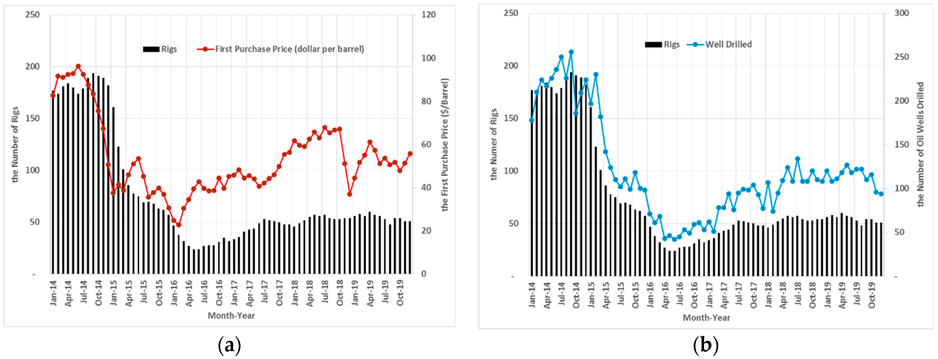
Figure 1. U.S. oil basins and major shale plays [5,6].
Infrastructures 06 00015 g001
Figure 2. Active oil wells and the number of rigs in operation: (a) the number of rigs and the first purchasing price and (b) the number of rigs and the number of wells drilled in the Williston Basin [39].
Infrastructures 06 00015 g002
Figure 3. Aerial view of oil field and map of oil pads, wells, and their legs: sources of (a,b) from Google® and (c) from [38].
Infrastructures 06 00015 g003
Figure 4. The dynamics of susceptible, infected, and recovered spacing units for 50 years starting from 2015.
Infrastructures 06 00015 g004
Figure 5. Spatial distribution of the oil drilling locations over the years.
Infrastructures 06 00015 g005
Figure 6. Yearly number of drillings per space.
Infrastructures 06 00015 g006
Table 1. Root mean square errors (RMSE) of infected sites for different values of β and μ.
β0.0000190.0000200.0000210.0000220.000023
μ
0.100.5610.4910.3850.4010.701
0.150.4110.3480.3280.3520.502
0.200.2880.2870.2070.2980.311
0.250.3710.2970.3040.3500.392
0.300.6070.3560.3090.4230.515
Table 2. Actual number of infected sites and the number of infected sites predicted from the simulation with β = 0.000021 and μ = 0.20.
YearActualPredicted% Matched
2016324262 81%
2017424331 78%
2018453385 79%
Publisher’s Note: MDPI stays neutral with regard to jurisdictional claims in published maps and institutional affiliations.