Experimental and Numerical Studies on Thermally-Induced Slip Ratcheting on a Slope

Abstract

Mild temperature fluctuation of a material sitting on a slope may only cause a small slip, but a large number of the repeated temperature changes can amplify the magnitude of the overall slip and eventually bring an issue of structural instability. The slip accumulation starts from the minor magnitude and reaches the extensive level called “slip ratcheting”. Experimental evidence for such thermally-induced slip ratcheting is first provided in this work. It is implemented with an acryl sheet placed on an inclined wood with a mild angle; it is found that the temperature fluctuation of the acryl sheet causes the sheet to slide down gradually without any additional loading. The numerical model is then attempted to emulate the major findings of the experiments. From the simulation work, the location of a neutral point is found when the acryl plate is heated, and another neutral point is observed when cooled down. The shift of the neutral point appears to be a major reason for the unrecovered slip after a temperature increase and decrease cycle. Finally, a parametric study using the numerical model is carried out to examine which parameters play a major role in the development of residual slips.

1. Introduction

Temperature fluctuation can cause various structural integrity problems at several different scales. Extreme heat can alter material properties by rearranging molecular structures, but even less severe temperature change can cause thermal cracking or buckling, as the material tends to expand and contract. Those temperature effects are relatively well-studied, but recently, some other cases were reported, which indicate moderately mild temperature change still could induce structural failure of the system—a slip accumulation (or allegedly “slip ratcheting”) over the interface between dissimilar materials accompanied with gravity. Examples of cyclic temperature and the corresponding displacement buildup of geotechnical systems are found in a variety of geotechnical problems, such as movements of natural rock slopes [1,2,3], exposed geosynthetic liners [4], pavement layers [5], and geothermal energy piles [6,7].

There are several common points in all these examples. First, a range of temperature change is not severe, so that the original material characteristics do not depreciate. Second, the interface slip corresponding to one temperature cycle is minor but continuously progresses as the number of cycles grows. Third, the whole system is equilibrated and stable before the temperature change, which means that an object on a slope has sufficiently large friction against the sliding. These points say temperature-caused interface slip accumulation can happen in any condition as long as two substances bear relatively different thermal expansion coefficients under continuous temperature changes. It also leads to the point that the traditional sliding stability analysis (i.e., $\mu >\tan \beta$, where $\mu$ is a frictional coefficient and $\beta$ is slope angle) may not be good enough to assess the long-term effect, especially under temperature fluctuation condition.

Unfortunately, there are not much reported observations of such slip ratcheting in many disciplines that can be used for in-depth follow-up study. Thermally-induced slip accumulation was first introduced for glacier slide by [8] and then a similar idea was later improved very recently by [5] for a pulsatile motion of pavement on the slope. On the other hand, geomembrane placed on construction slope also has been observed to experience thermal expansion and contraction (e.g., [9,10]); and Ref. [4] performed a lab test to see a geomembrane slippage over a slope. Ref. [2] attested that a slip accumulation indeed occurred in a field condition based on a field observation regarding the irreversible slip of a granite rock slab movement and estimated the future slippage with a numerical study.

All of these studies, however, use slightly different terminologies, ranging from “pulsatile motion [5]”, “crawling theory [11]”, “insolation creep [5]”, to “displacement ratcheting [12]”, which discloses there has not been sufficient study carried out to see the fundamental mechanism of “slip ratcheting” features. There is a clear need for future theoretical, numerical, and experimental work to extend their simple but robust approaches. Suggested future work includes more precise theoretical solutions, more realistic numerical simulations, carefully planned experimental investigations, and automated monitoring of displacements and temperatures of rock blocks at fields [2,5].

Most recently, [13] also suggested experimental evidence and a numerical algorithm on the thermal ratcheting problem. However, we still lack a fundamental understanding of the phenomena itself, and how it is affected by several influential parameters. In this regard, this study attempts to provide controlled experimental evidence and a numerical simulation approach for the study of thermally-induced displacement ratcheting. The produced work from this study helps reveal the fundamental features of the displacement ratcheting at an interface that can be expanded to the sustainable design of geostructures, such as geothermal energy piles, buried pipelines, exposed geosynthetic liners, and pavement layers, as well as the reliable prediction of the movement of natural rock slopes.

2. Experimental Observation

Experimental demonstration of the slip ratcheting is an essential part of this study as there are no sufficient studies in the literature, especially in a controlled condition. The experiment outcome obtained here can be utilized for both the evidence of slip ratcheting and the validation of the numerical simulation later. In this experiment, the material placed on the slope will undergo a number of heating–cooling cycles, and it is expected to continuously slide down with the number of cycles, that is, the slip ratcheting.

2.1. Slope Test

An overall test setup is shown in Figure 1a: an acryl plate sits on an inclined wood slope with an inclination angle of $\beta$, and a heating pad is attached on the top of the acryl plate (Figure 1b). The inclination angle was selected to be $\beta =5°$ and $10°$, so that the acryl plate does not slide down by gravity only—the critical inclination angle is around $15°$ (see

Table 1. List of thermoelastic properties of the acryl and the acryl-wood interface.

Properties	Values
$\mathrm{Young}’\mathrm{s} \mathrm{modulus} \mathrm{of} \mathrm{acryl}, E$*	$3.1 \mathrm{GPa}$
$\mathrm{Poisson} \mathrm{ratio} \mathrm{of} \mathrm{acryl}, \nu$*	0.37
$\mathrm{Density} \mathrm{of} \mathrm{acryl}, \rho$*	$1.19 \mathrm{g}/{\mathrm{cm}}^3$
Linear thermal expansion coefficient of acryl$, \alpha$*	$7\times {10}^{-5} {\mathrm{K}}^{-1}$
Linear thermal expansion coefficient of wood$, \alpha$*	$5\times {10}^{-6} {\mathrm{K}}^{-1}$
$\mathrm{Friction} \mathrm{coefficient} \mathrm{at} \mathrm{acryl}-\mathrm{wood} \mathrm{interface}, {\mu }^{ **}$	0.271
$\mathrm{Elastic} \mathrm{limit} \mathrm{at} \mathrm{acryl}-\mathrm{wood} \mathrm{interface}, \delta { }^{**}$	$0.01 \mathrm{mm}$

* adopted from www.matweb.com (material property data webpage). ** determined by conducting direct shear tests in this study.

). The acryl and wood materials are chosen to have a significant difference between thermal expansion coefficients of two materials (i.e., coefficients of linear thermal expansion are $~7\times {10}^{-5} {\mathrm{K}}^{-1}$ for acryl vs. $~5\times {10}^{-6} {\mathrm{K}}^{-1}$ for wood) and to minimize buckling or wrinkling effect when stretched. The dimension of the acryl plate is $12.7 \mathrm{cm}\times 7.6 \mathrm{cm}\times 0.25 \mathrm{cm}$ (length $\times$ width $\times$ thickness). Other thermo-elastic properties of the acryl are summarized in Table 1. The electric heating pad, attached on the top of the acryl plate, is connected to a power supply and a switch that turns on-and-off for a designated time interval.

For the experimental demonstration, we applied the voltage of the power supply as $5 \mathrm{V}$ and $6 \mathrm{V}$ with the on-and-off time interval of the power supply as $10$ min for the total experiment time of $12$ h (i.e., total $36$ heating–cooling cycles) (Figure 1c). Ten minutes of the heating–cooling duration is found sufficiently long to attain the consistent temperature at the acryl plate. During the test, the movement of the acryl plate was monitored using time-lapse photography (photo interval of $15$ s) (Figure 1d). With the described test conditions (i.e., $5 \mathrm{V}$ and $6 \mathrm{V}$ of power supply for heating and $5°$ and $10°$ of the inclination angles), a total of 4 different cases are examined, and each case is performed twice for reproducibility. The amplitudes of temperature fluctuation are observed to be about $23 °\mathrm{C}$ and $31 °\mathrm{C}$ for $5 \mathrm{V}$ and $6 \mathrm{V}$ of applied powers, respectively (starting temperature is about $29 °\mathrm{C}$) (Figure 1c). There is no additional external force applied other than the temperature fluctuation during the tests. The accumulated slip is measured from the analysis of captured images of the acryl plate by the time-lapse camera, assuming the underlying wood slope is neither deforming nor moving.

For all conditions of the experiments, it is observed the slip values of the acryl plate over the wood slope are continuously growing. The amounts of slip are different, but they all linearly increase as the temperature fluctuation cycle continues. In general, the amount of accumulated slip becomes greater with a higher amplitude of temperature change and a larger inclination angle. The accumulated slip magnitudes are ranging from $1.075 \mathrm{mm}$ ($\Delta T=23 °\mathrm{C}$ in $\beta =5°$ slope) to $2.910 \mathrm{mm}$ ($\Delta T=31 °\mathrm{C}$ in $\beta =10°$ slope) after the 36 cycles. There are minor discrepancies in the results from the same experimental condition (i.e., same $\Delta T$ and $\beta$), but the overall tendency of the test results is consistent. As the slip increase is observed to be linear, the slip values after extended cycles can also be predicted via extrapolation of the first 20 cycles or so. In summary, the experimental results help to ascertain the ratcheting behavior of the slip growth and imply that the amount of slip will never be reduced down later (Figure 2).

2.2. Direct Shear Test

In parallel to the slope tests, direct shear tests (equipment: DigiShear^TM by GeoTac) are conducted to identify the fundamental behavior of interfacial shear between the acryl plate and the wood slope and, thus, to understand the mechanism of the thermally-induced slip ratcheting more in-depth. The direct shear-type test is one of the popular geotechnical test methods for the evaluation of shear strength at the interface of materials in circular-upper and lower shear boxes (ASTM D3080 [14]). For this study, the same wood material is housed in the lower shear box, and the acryl is housed in the upper shear box (outer diameter: $63.5 \mathrm{mm}$). Once the two materials are in each shear box and are in contact, the normal stress is applied by the vertical actuator. A series of direct shear tests were performed under the various range of normal stresses, from $2.5$ to $200 \mathrm{kPa}$, to evaluate the shear strength parameters. Note that the actual magnitude of the normal stress imposed on the acryl plate during the slope test is very small, about $29 \mathrm{Pa}$, only by the self-weight of the acryl plate. During the test, the acryl plate is horizontally pushed by the other actuator with the shear rate at $0.05 \mathrm{mm}/\min$ under the constant normal stress condition. The horizontal displacement of the shear box and the applied horizontal force are monitored during the test for analyzing the shear strength parameters at the acryl-wood interface. When the shear stress reaches the maximum value and then remains constant, the test is terminated.

Shear strength at the interface can be defined by a set of shear strength parameters—the coefficient of friction ($\mu$) and the elastic limit ($\delta$) of interface shear displacement (Figure 3). As shown in the plot of shear stress vs. displacement relationship, the interface shear behavior can be approximated with an elasto-perfectly-plastic constitutive model. The coefficient of friction ($\mu$) remains practically constant over the entire range of the normal stress (Figure 4a), but the elastic limit ($\delta$) is observed to be highly dependent on the normal stress (Figure 4b). The elastic limit for the condition of the slope test in this study is determined to be about ~0.01 mm based on the extrapolation of the observed elastic limits to the actual normal stress of $~29 \mathrm{Pa}$. The interface strength parameters are also summarized in Table 1.

3. Numerical Study—Comparison with Experiment

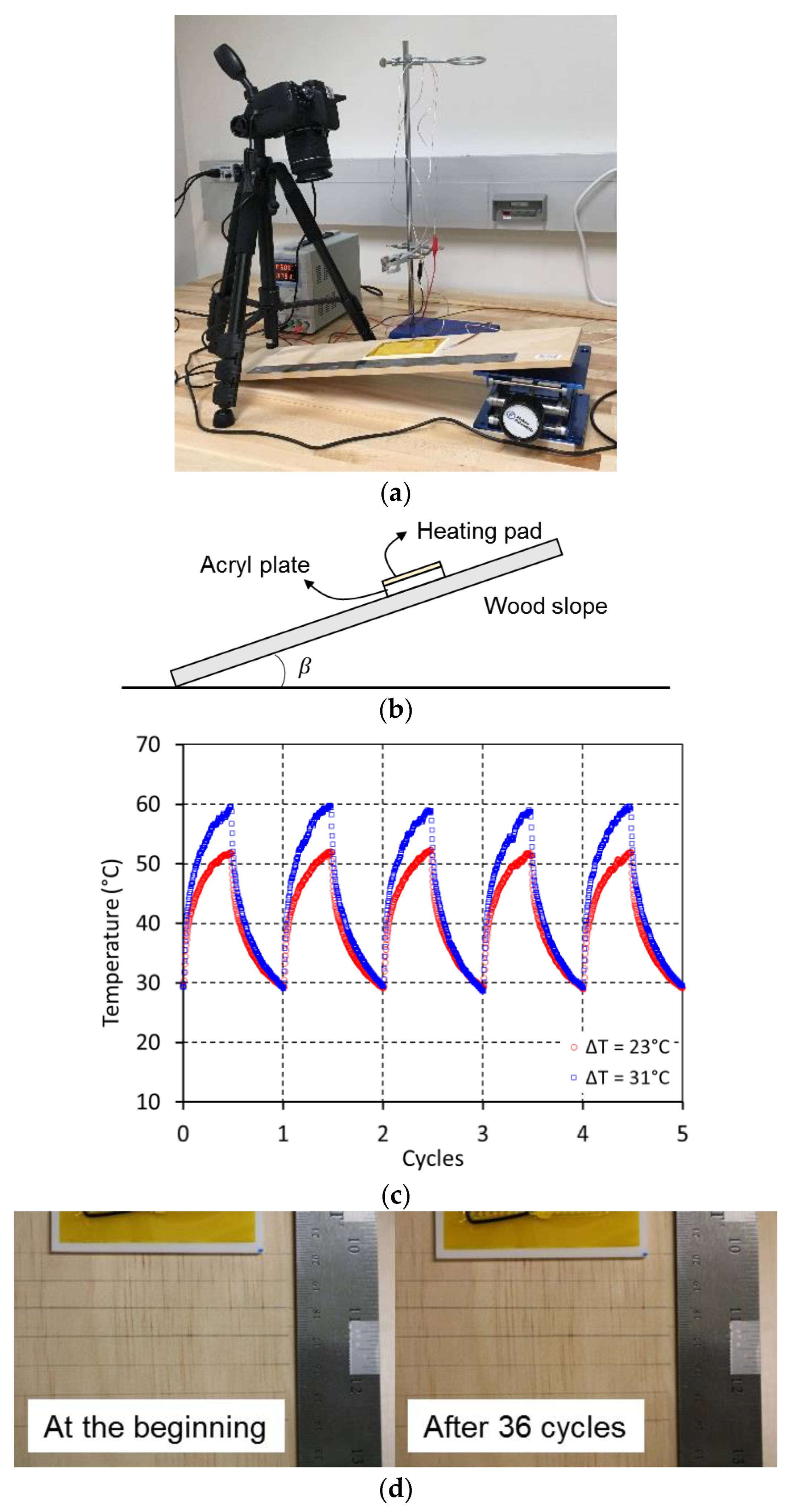
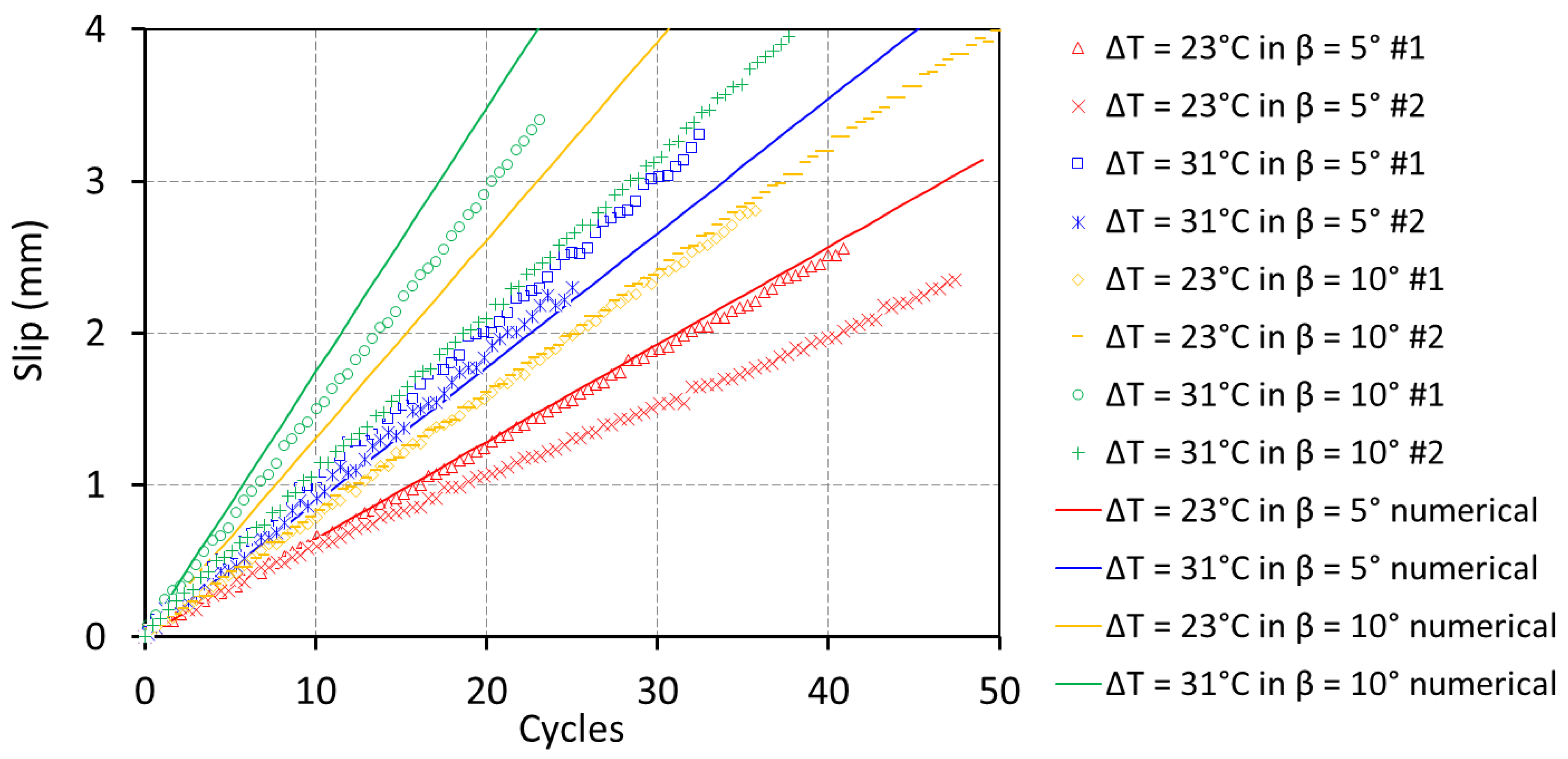
Experiments reveal that the acryl plate gradually slides down (i.e., slip accumulation) only with the temperature variations. Even though the simple experiment can demonstrate the actual occurrence of slip ratcheting even under mild temperature changes, it is still not clear how the slip between two materials continuously grows and how much amount of the slip can be estimated after a large number of cycles. Moreover, there is a practical limitation of the number of temperature cycles that can be applied during the experimental study (e.g., the presented experimental work takes 12 h to monitor a gradual slip ratcheting over 36 cycles). In this respect, numerical analysis or analytical approach that can reproduce the described experimental results would be a great alternative, which will enable us to explore a much larger number of cycles.

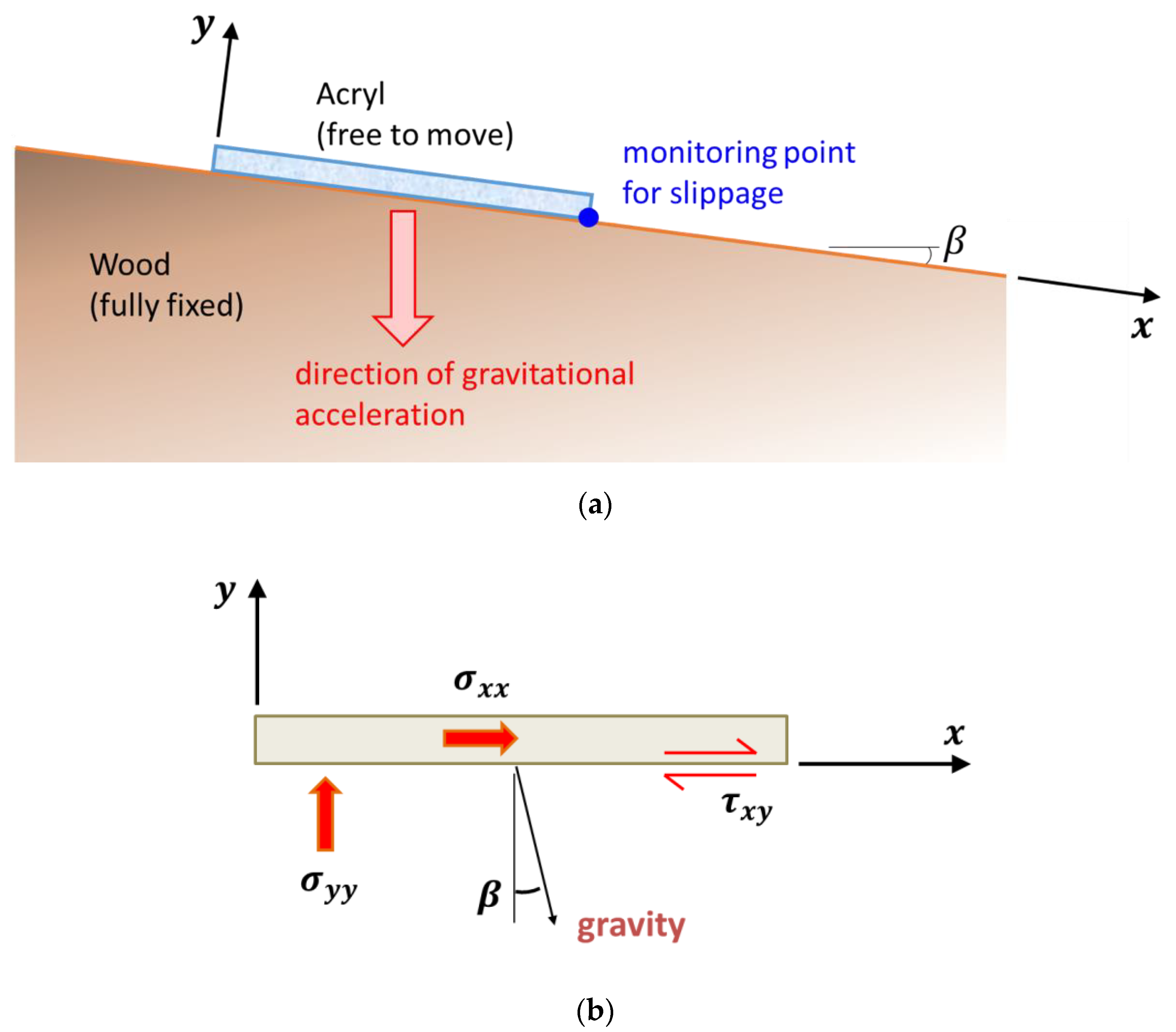
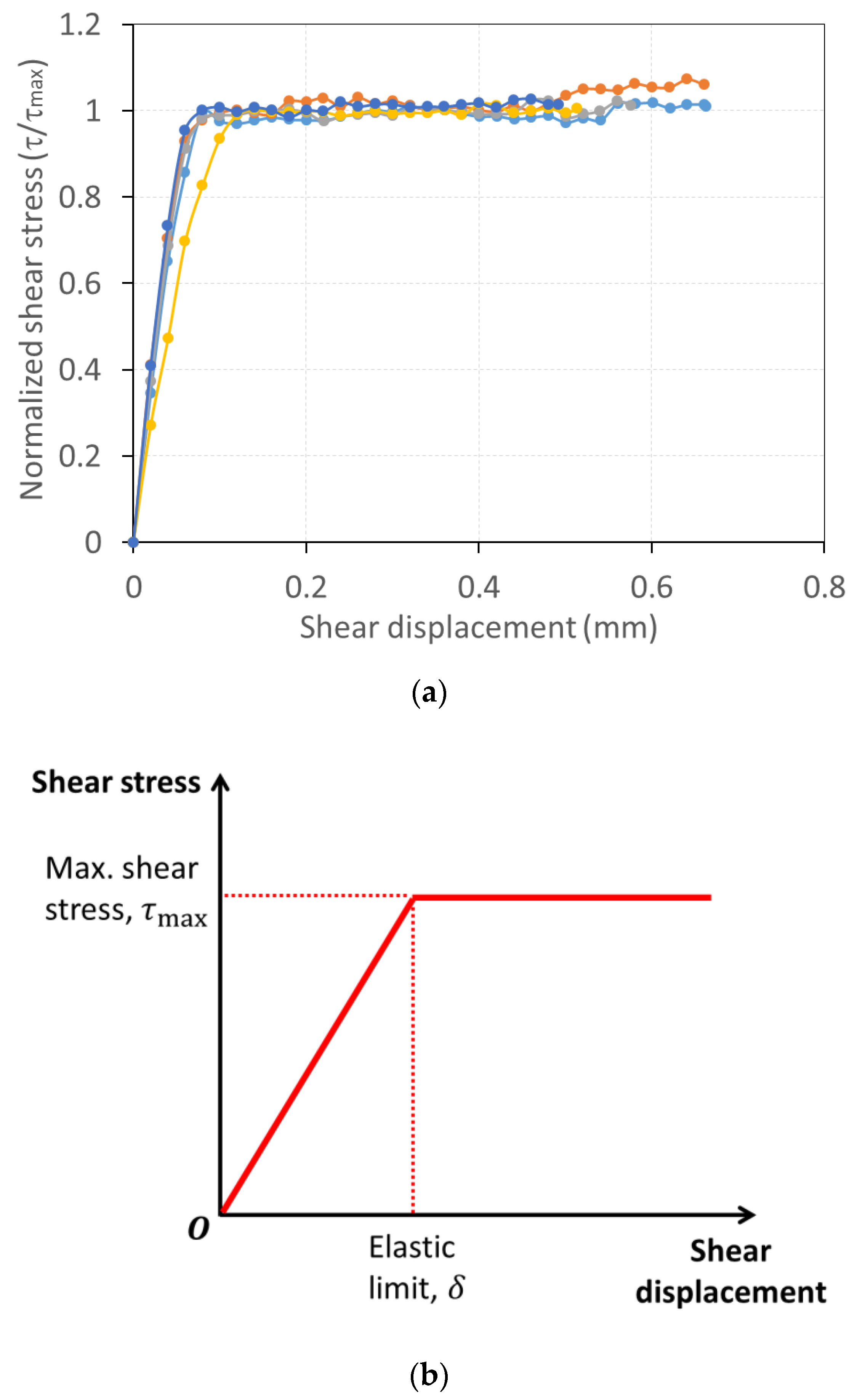
The finite element model is constructed accordingly in the plane strain condition using Abaqus (Figure 5a). Note that a comparison between the two-dimensional plane strain and three-dimensional simulations is discussed in a later section. The acryl and wood in the simulation model are set as linear elastic materials with the representative mechanical and thermal properties listed in Table 1. The interface is treated as linear elastic-perfectly plastic using the Coulomb frictional model. The coefficient of friction ($\mu$) and the elastic slip ($\delta$) are applied to the interface of those two materials. The wood is assumed not to deform against gravity nor temperature fluctuations, thus fully fixed in all directions, whereas the acryl plate as a sliding slab is not constrained at all. Similar to the experiment, the acryl plate is placed on the wood slope inclined at an angle of $\beta$, and only a gravitational acceleration is applied. Then, the temperature of the acryl plate is increased by $\Delta T$ and then decreased by the same temperature change ($\Delta T$). The combination of temperature increase and decrease of the acryl plate is deemed one cycle of temperature fluctuation, and up to 50 temperature cycles are applied to the acryl plate during the numerical simulation. Similar to the experimental conditions, two cases of temperature changes ($\Delta T=23 °\mathrm{C}$ and $31 °\mathrm{C}$) and two cases of the inclination angles ($\beta =5°$ and $10°$) are considered in the simulations for comparison with the experimental outcomes. The slip accumulation is monitored at the front end of the acryl plate (Figure 5a). Moreover, the stress values, along with the slip, are to be presented in the next section (following the definitions in Figure 5b). That is, ${\sigma }_{xx}$ is the normal stress acting parallel to the slope surface, ${\sigma }_{yy}$ is the normal stress acting perpendicular to the slope surface, and ${\tau }_{xy}$ is the shear stress between the acryl and the wood. All of these stress values are monitored at the base of the acryl. The positive normal stresses represent tensile values as per traditional mechanics and the negatives are for compressive ones. The positive shear stress denotes downward shear stress on the acryl side, which is the same as the one shown in Figure 5b.

Here are several simplifications made for the numerical works. First, material strength degradation with repetitive/cyclic thermal loading is not considered here. That is, the interface strength between the acryl and wood assumed to have the same magnitude throughout the temperature cycles indefinitely. Moreover, although temperature increases at gradually decreasing rates during the experiments (blue squares in Figure 6a), it changes linearly in the simulation conditions (red dotted line in Figure 6a). Moreover, in the experiments, the acryl is heated from the top where the heating pad is attached, which might cause a minor temperature gradient inside the acryl; but the uniform temperature increase of the entire acryl plate is applied in the simulation. Finally, the acryl sliding is, rather, a three-dimensional feature, but the model described above uses a two-dimensional plane-strain condition. All simplifications made here are discussed further in the discussion section.

For a better representation of the numerical result, the “residual values” of the slips (solid red line in Figure 6b) are primarily examined here instead of the entire trace of the fluctuating slips (dotted red line in Figure 6b) with the temperature fluctuation. The “residual values” are the slip magnitudes after the temperature of the plate ($\Delta T$) drops back to its initial temperature. In this way, the numerical result can be presented as simple straight lines instead of zigzag lines.

Comparisons of the experimental outcomes and the numerical results are summarized in Figure 7. The accumulated slip values after 20 cycles range from $1.245 \mathrm{mm}$ ($\Delta T=23 °\mathrm{C}$ in $\beta =5°$ slope) to $3.485 \mathrm{mm}$ ($\Delta T=31 °\mathrm{C}$ in $\beta =10°$ slope). These are somewhat close to that of the experiments ranging from $1.075 \mathrm{mm}$ ($\Delta T=23 °\mathrm{C}$ in $\beta =5°$ slope) to $2.910 \mathrm{mm}$ ($\Delta T=31 °\mathrm{C}$ in $\beta =10°$ slope). Apparently, there are certain discrepancies in the magnitudes of the accumulated slips. Nonetheless, the experimental outcomes and the numerical results can be regarded to be reasonably in good agreement in the aspect that the slip values all consistently and linearly increase, and the errors between the experiment and the simulation results are comparable to those between two experimental tests at the same condition.

Numerical Study—Slip Behavior

Upon the verification of the numerical model used for the thermally induced slip ratcheting in the previous section, the model now can be used to examine further how the interface strengths are mobilized during the slip ratcheting. We particularly focus on stress components and slip values at the interface in this section. The aim is to offer a better understanding of the behavior of the interface and the slip accumulation during temperature fluctuation. The coordinates for the stress components are shown in Figure 5b; the axis parallel to the slope is $x$-axis, and the one perpendicular is $y$-axis.

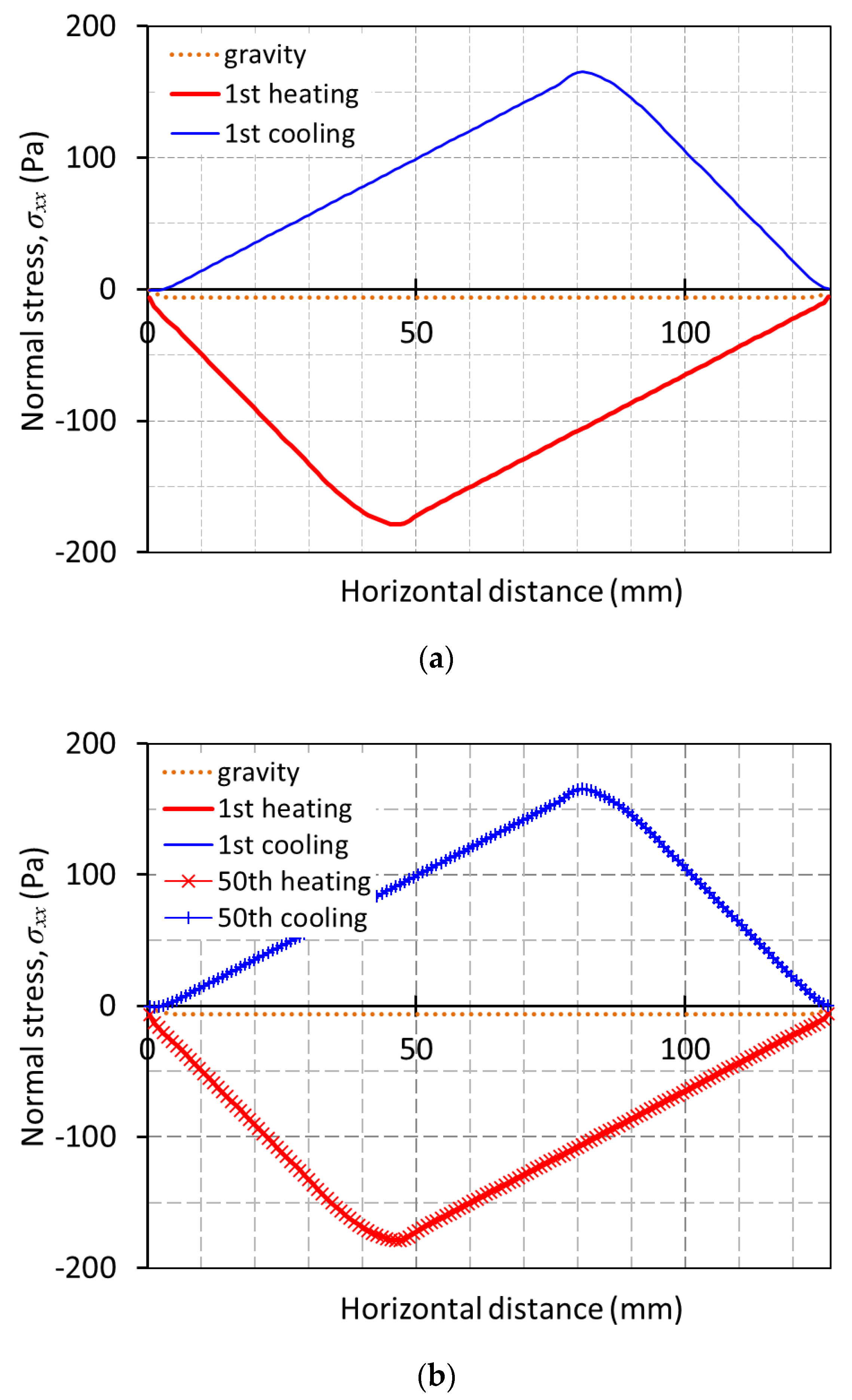
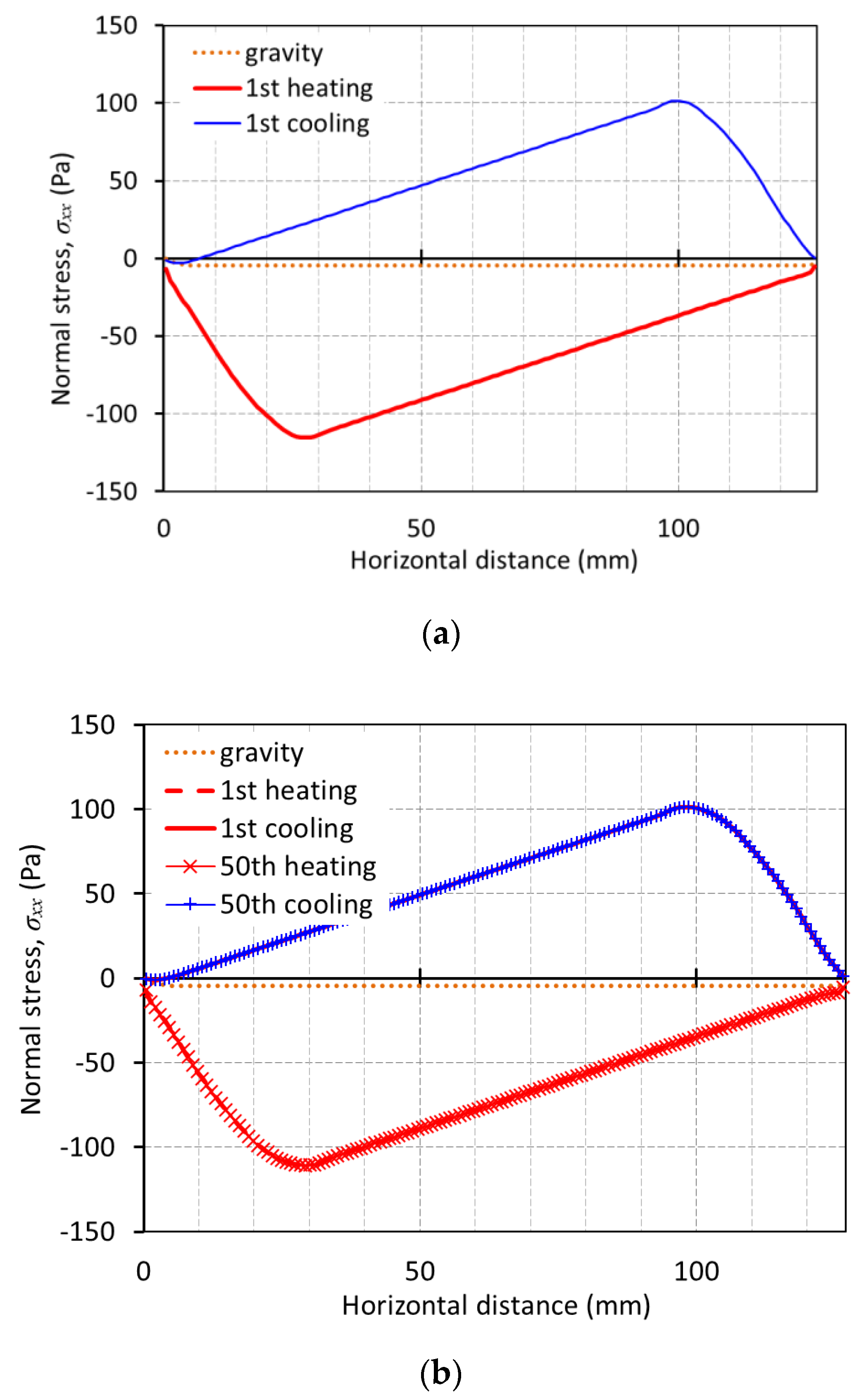
First, the distributions of normal stress in a direction parallel to the slope surface (${\sigma }_{xx}$) on the acryl plate are shown in Figure 8. Normal stress with gravitational loading only is presented as a dotted-orange line (Figure 8), which magnitude is much smaller than that when any temperature changes are imposed. The distribution of normal stress with gravity appears nearly uniform, and the magnitude is around $-4.2 \mathrm{Pa}$. With a temperature increase (labeled as “heating”), the distribution of normal stress (${\sigma }_{xx}$) becomes negative (compressive), non-uniform, and concave-up with approximately $-175 \mathrm{Pa}$ of the peak at around $46 \mathrm{mm}$ from the left end and nearly $0 \mathrm{Pa}$ at both left and right ends of the acryl plate (a red line in Figure 8a). It implies that, when the acryl is heated, the entire acryl plate is under compressive stresses, caused by the constraint of the frictional resistance between the acryl and the wood, namely, interface shear strength against thermal expansion behavior.

Once the temperature of the acryl drops back to the initial value (labeled as “cooling”), the normal stress (${\sigma }_{xx}$) becomes positive (tensile) and its distribution in the plate is concave-down with the peak of $~166 \mathrm{Pa}$ around $81 \mathrm{mm}$ from the left end of the acryl plate (a blue line in Figure 8a). In contrast to the heating cycle, the entire acryl plate is under tensile stresses with the temperature drop, and this is because the shrinkage of the acryl plate is obstructed by the interface shear stress. It is also observed that the distribution shapes and the stress magnitudes do not change as the temperature cycle continues. For instance, the distributions at the 50th cycle of temperature fluctuation are essentially the same as those of the first cycle (Figure 8b; the distributions at the first and 50th cycles are completely overlapped). With such a constant distribution of normal stresses, we can postulate that the locations of the maximum and the minimum normal stresses (i.e., $81 \mathrm{mm}$ and $46 \mathrm{mm}$ from the left end, respectively) are approximately the “neutral points”. This will be discussed further in the next paragraph.

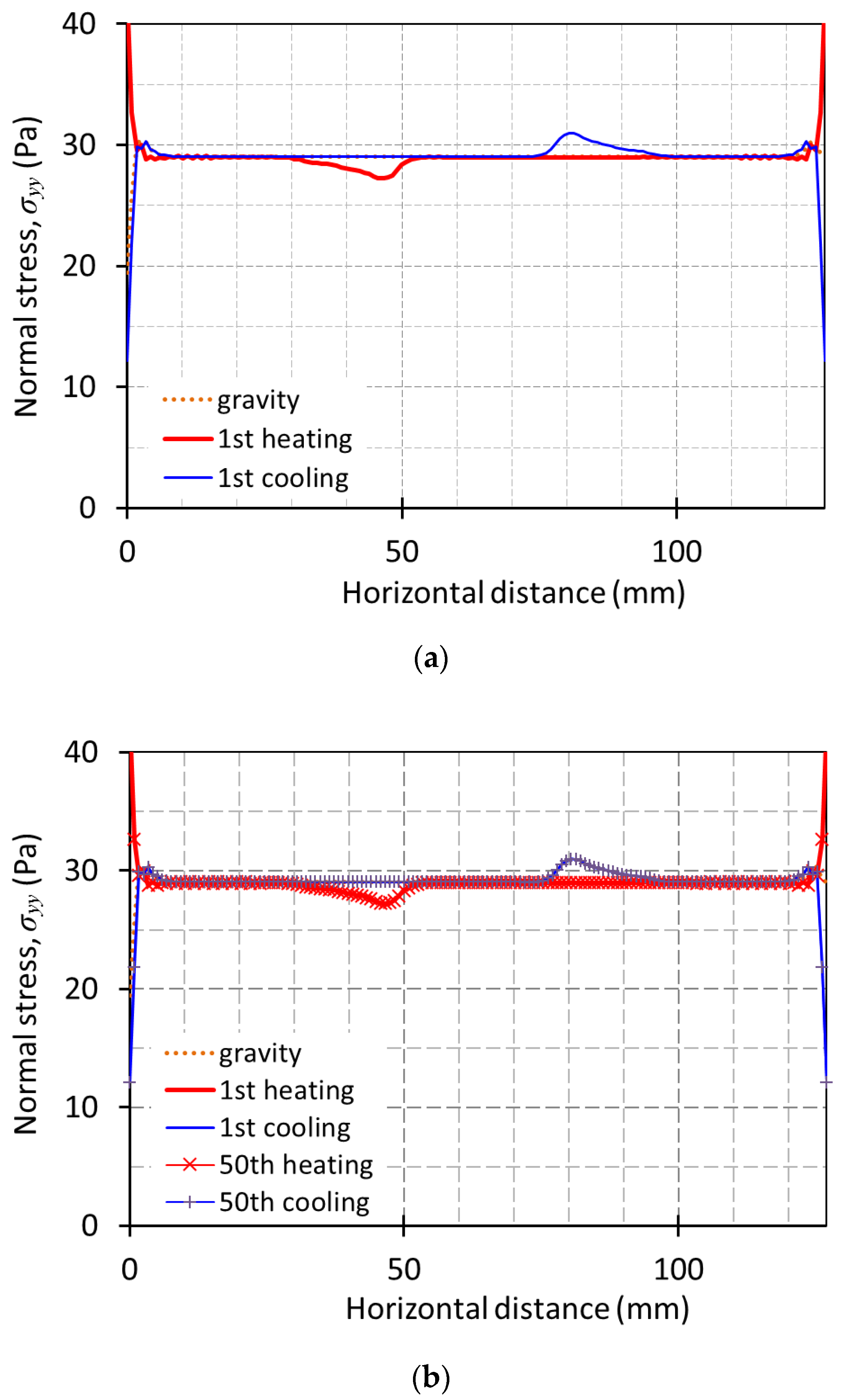
The distributions of normal stress in a direction perpendicular to the slope surface (${\sigma }_{yy}$) at the base of the acryl plate is shown in Figure 9. Similar to ${\sigma }_{xx}$ in Figure 8, the distribution shapes and the stress magnitudes of ${\sigma }_{yy}$ also do not change during the 50 cycles of heating–cooling. The magnitude of ${\sigma }_{yy}$ with gravitation loading only also more or less the same as those with temperature increase or drop, which is approximately $29 \mathrm{Pa}$, the value calculated in Section 2.2. There are small disturbances observed when the acryl is heated and cooled down; the amplitudes are up to $2 \mathrm{Pa}$, which is much smaller than the base value ($29 \mathrm{Pa}$). The locations of the disturbances of ${\sigma }_{yy}$ coincide with the location of the peak ${\sigma }_{xx}$ values, (i.e., $81 \mathrm{mm}$ and $46 \mathrm{mm}$ from the left end, respectively).

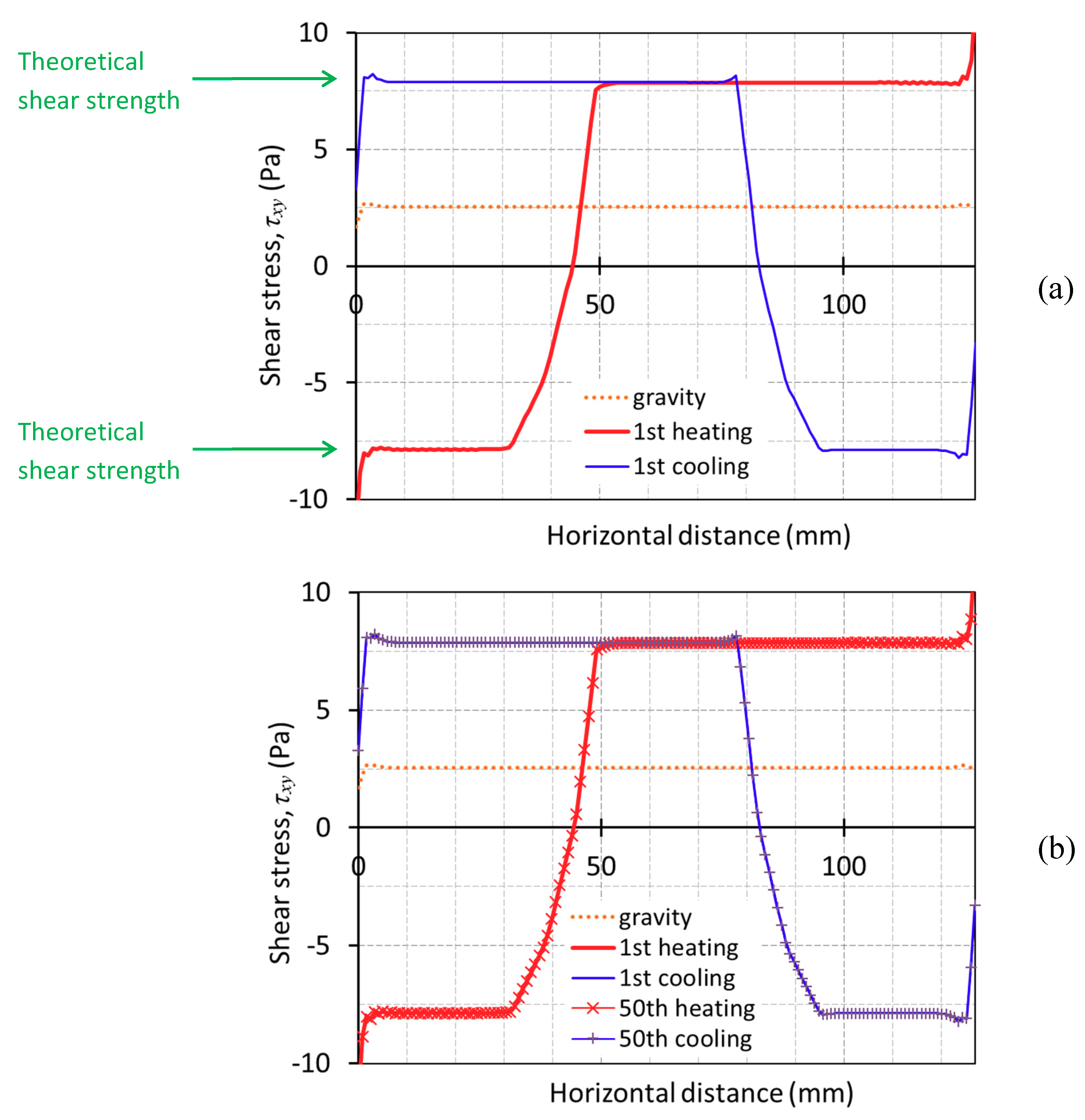
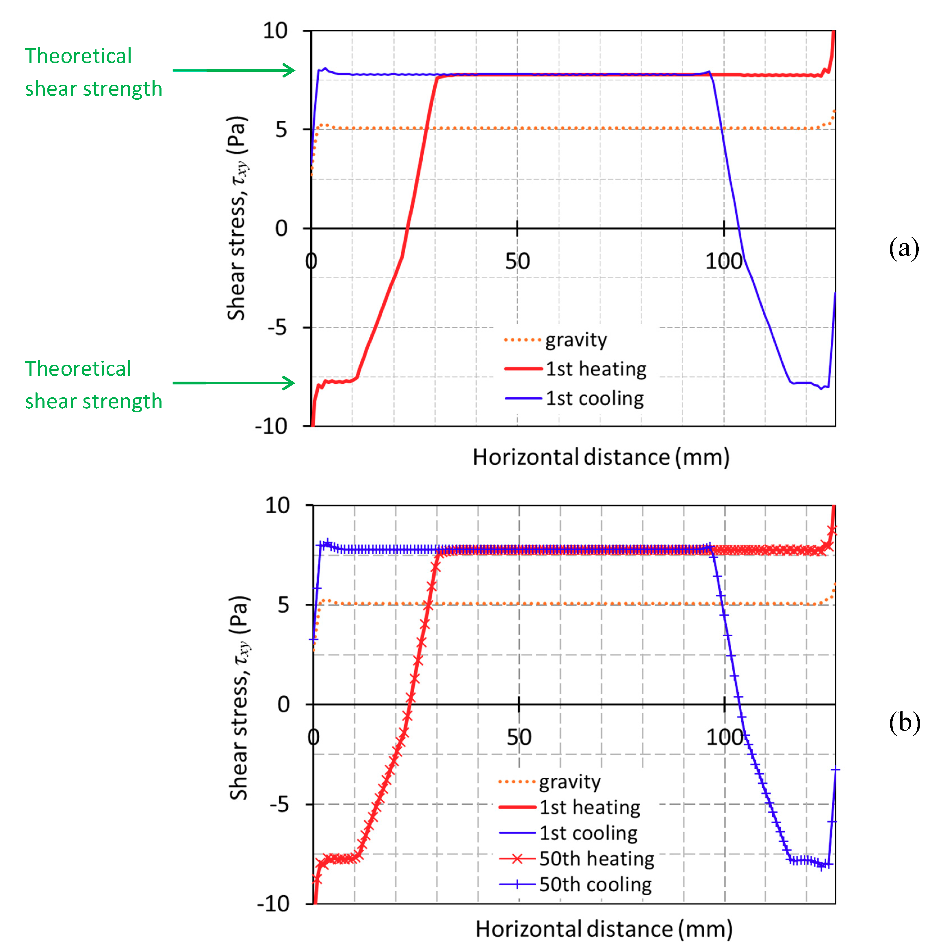
The distributions of interface shear stress (${\tau }_{xy}$) at the acryl-wood interface are presented in Figure 10. Note that shear stress is positive for the downslope direction and negative for the upslope at the lower surface of the acryl plate. Shear stress only with the gravitational loading is also plotted in Figure 10 (a dotted orange line), which appears nearly uniform and small in magnitude (~$2.5 \mathrm{Pa}$). With a temperature increase (“heating”), the shape of interface shear stress distribution is similar to a step function with a slanted jump from the minimum to the maximum (a dashed line in Figure 10a). The maximum and minimum values of shear stresses are nearly the same with the different signs, which implies that the interface shear stress reached its shear strength of ${\tau }_f=7.879 \mathrm{Pa}$ (note that ${\tau }_f=\mu \rho gh\cos \beta =0.271\times 1.19\frac{\mathrm{g}}{{\mathrm{cm}}^3}\times \frac{9.81\mathrm{m}}{{\mathrm{s}}^2}\times 0.25 \mathrm{cm}\times \cos 5°=7.879 \mathrm{Pa}$). Therefore, over the interval of $0 \mathrm{mm}$ and $30 \mathrm{mm}$ (from the left end, hereafter), the interface shear stress is approximately constant of $-7.879 \mathrm{Pa}$, and over the interval of $51 \mathrm{mm}$ to the right end, it is constant $7.879 \mathrm{Pa}$. Between $30 \mathrm{mm}$ and $51 \mathrm{mm}$, the shear stress monotonically increases with zero at around $44\mathrm{mm}$. Therefore, it can be inferred that a part of the acryl plate from the left end to $44 \mathrm{mm}$ deforms upwards while the remaining part from $44 \mathrm{mm}$ to the right end deforms downwards. Thus, the location of $44 \mathrm{mm}$ can be considered as the “neutral point” when the acryl plate is heated, which is very close to $46 \mathrm{mm}$ (determined from the normal stress distribution). Therefore, the estimate of $44 \mathrm{mm}$ (determined from the shear stress distribution) is deemed as a more accurate one.

With the temperature drop (“cooling”), the shape of interface shear stress distribution is flipped over (a solid line in Figure 10b) from that of the heating cycle, but with the different intervals for the maximum and minimum shear stresses. The interface shear stress is almost constant of $7.879 \mathrm{Pa}$ over the interval of $0 \mathrm{mm}$ and $77 \mathrm{mm}$, and it is again constant at $-7.879 \mathrm{Pa}$ over the interval of $98 \mathrm{mm}$ to the right end. Between $77 \mathrm{mm}$ and $98 \mathrm{mm}$, the shear stress decreases monotonically with zero at around $83 \mathrm{mm}$. Similar to the heating cycle, the location of $83 \mathrm{mm}$ can be considered as the “neutral point” when the acryl plate is cooled down ($81 \mathrm{mm}$ from the normal stress distribution). Moreover, like the normal stress distribution, the distribution of interface shear stress remains the same during the 50th temperature cycles, which implies the stress conditions will not change hereafter.

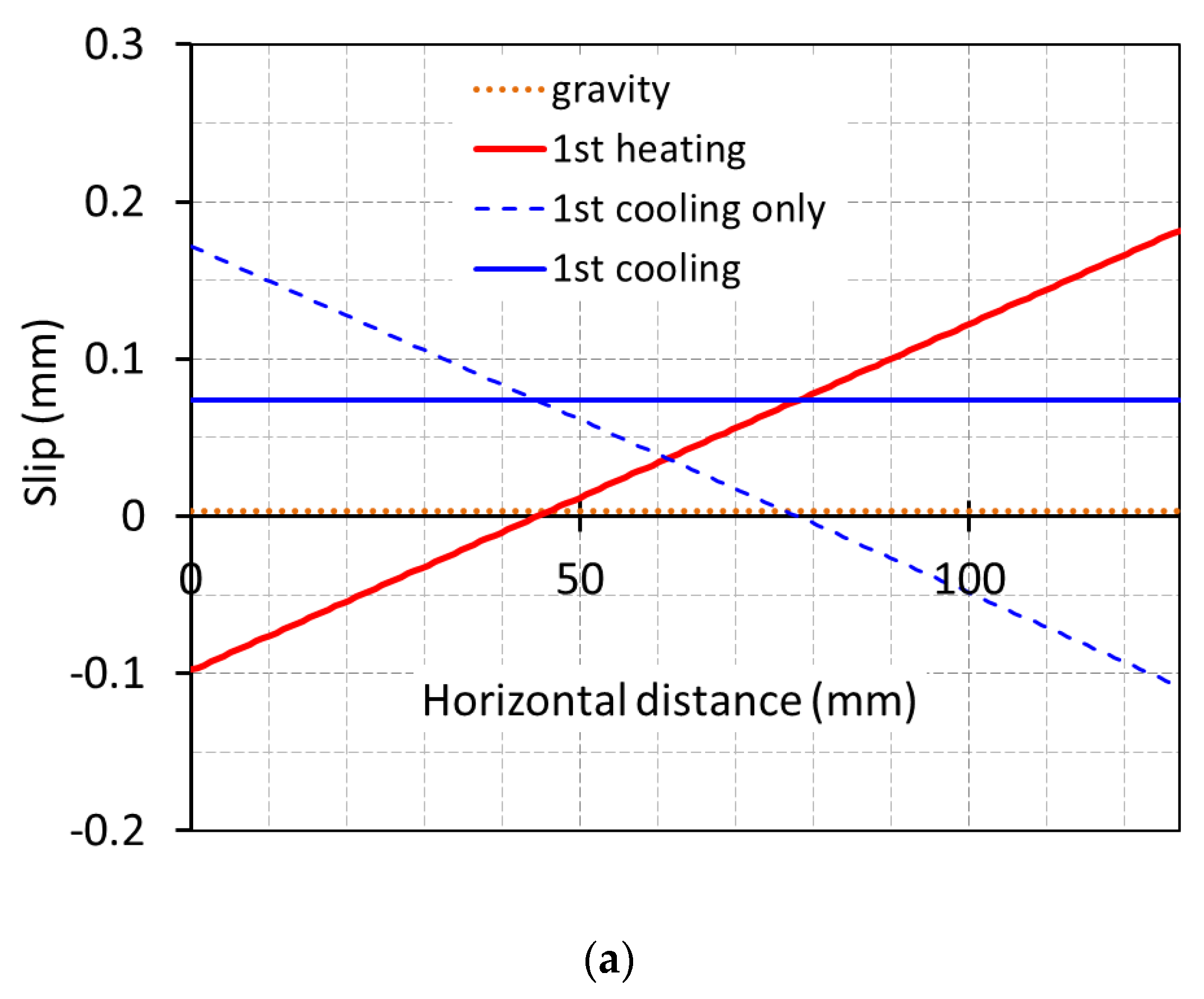
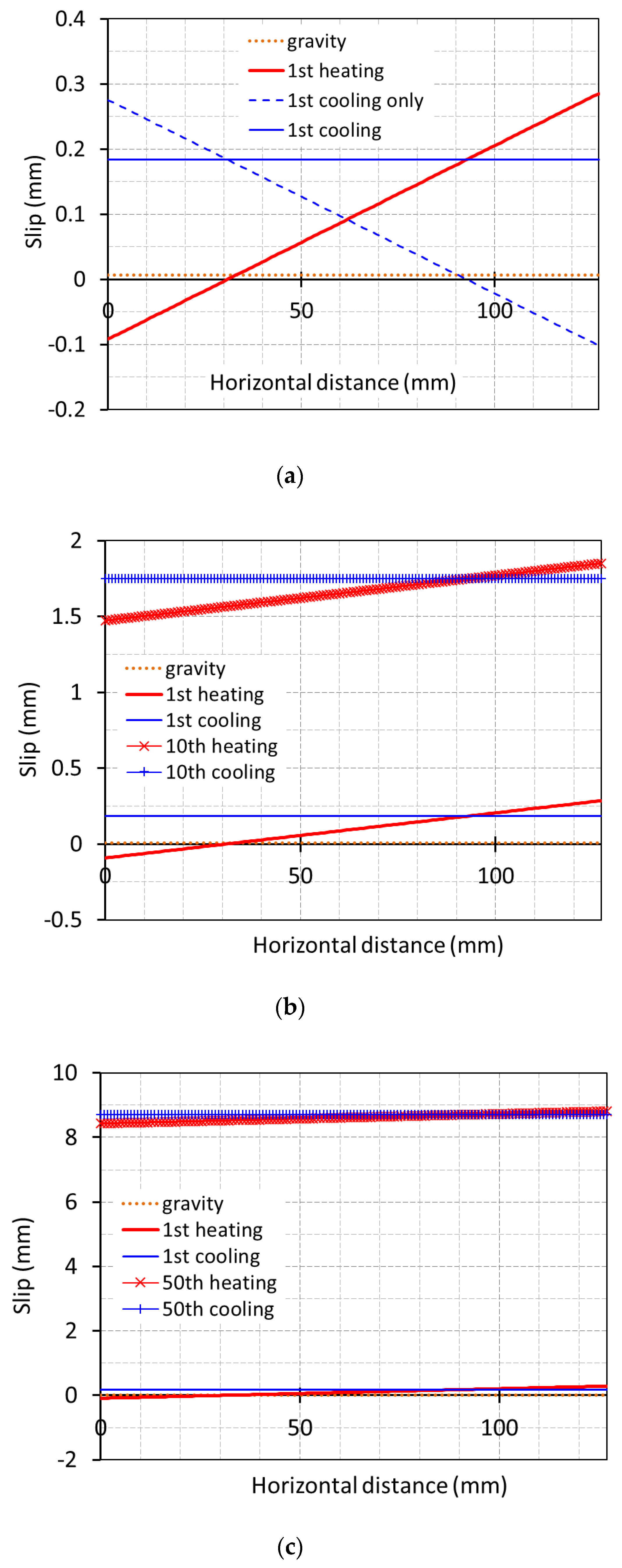
The distribution of the interface slips at the acryl-wood interface is described in Figure 11. Positive values of the slip denote the downhill direction, whereas negative ones for the uphill movement. Slip by the gravitational loading only is negligible, as shown in Figure 11a (a dotted line; approximately $3.23 \mathsf{\mu }\mathrm{m}$). When the temperature is increased, the slip distribution at the interface is linear, from $-0.070 \mathrm{mm}$ to $0.13 \mathrm{mm}$ (from the left end to the right, a dashed line in Figure 11a). The location of zero slip appears to be approximately $44 \mathrm{mm}$, which coincides with the neutral point identified from the interface shear stress distribution (Figure 10). When the acryl plate is cooled back, the slip distribution is flipped over from $0.124 \mathrm{mm}$ to $-0.080 \mathrm{mm}$ (from the left end to the right, a dot-dash line in Figure 11a), which shows another neutral point at $77 \mathrm{mm}$. The overall distribution of the slip after the combined heating–cooling cycle is approximately constant at $0.074 \mathrm{mm}$ (a blue solid line in Figure 11a), which is fundamentally an irrecoverable, residual slip that is also shown in Figure 6b and Figure 7.

There is a major difference found between the stress distributions (i.e., normal and shear) and the slip distribution; the slip distribution has an increasing magnitude with the repetition of the temperature cycle, whereas the stress distribution does not. As noted earlier, the same stress distribution shape during the temperature cycles implies that the locations of the neutral points are the same. The irrecoverable slip occurs even from the first heating–cooling cycle, which implies that the slip will continue to accumulate as the temperature cycle repeats. Moreover, the magnitude of the irrecoverable slip at each heating–cooling cycle must be the same, given that the stress values are identical during all the cycles. Therefore, the irrecoverable slip will continuously grow with the temperature cycles, and it should be linearly growing. For instance, the irrecoverable slip is $0.003 \mathrm{mm}$ with the gravity, $0.074 \mathrm{mm}$ at the first cycle, $0.646 \mathrm{mm}$ at the 10th cycle, and then $3.213 \mathrm{mm}$ at the 50th cycle (solid lines in Figure 11b,c), which is approximately $0.064 \mathrm{mm}/\mathrm{cycle}$.

Similar features are also found in the different case with the higher temperature amplitude and slope angle, $\Delta T=31 °\mathrm{C}$ in $\beta =10°$ slope (Figure 12 through Figure 13 and Figure 14). The overall patterns of the normal stress (${\sigma }_{xx}$), interface shear stress (${\tau }_{xy}$), and slip at the acryl-wood interface are found similar. However, the magnitudes of the stresses and the slips along with the neutral point positions are quite different from those from the previous condition ($\Delta T=23 °\mathrm{C}$ in $\beta =5°$ slope). For example, the minimum normal stress is about $-110.7 \mathrm{Pa}$ around $29 \mathrm{mm}$ (from the left end hereafter) when heated, and the maximum value comes at about $101.3 \mathrm{Pa}$ around $98 \mathrm{mm}$ when cooled down (Figure 12). Zero interface shear stress is observed at around $23 \mathrm{mm}$ and $104 \mathrm{mm}$ when heated and cooled down, respectively, and the neutral points are identified as those locations accordingly. The intervals of the shear stress transition are between $8 \mathrm{mm}$ and $32 \mathrm{mm}$ and between $95 \mathrm{mm}$ and $119 \mathrm{mm}$ when heated and cooled down, respectively (Figure 13). Moreover, after the first heating–cooling cycle, the residual slip is $0.358 \mathrm{mm}$ ($0.184 \mathrm{mm}$ slip with gravity), and it accumulates to $1.744 \mathrm{mm}$ after 10 cycles, and to $8.717 \mathrm{mm}$ after 50 cycles, which is approximately $0.171 \mathrm{mm}/\mathrm{cycle}$ (Figure 14). Please be noted that the described features in the distributions of normal and stress forces and the slip values are also presented in [13] to some extent.

As shown in those two cases of simulations, the magnitude of a residual slip is affected by the location of the neutral points. It helps to consider an extreme case where the neutral point is exactly at the middle of the acryl plate: that is, when the acryl is placed on a flat surface ($\beta =0°$), then the neutral point is always at the half of the plate during both heating and cooling conditions. Intuitively, no irrecoverable slip is expected in this case. Therefore, the flip of the neutral point about the center of the plate during the heating-and-cooling cycles is believed to be a primary reason for such a residual slip. Moreover, the irrecoverable slip would increase as the distance from the neutral point to the middle of the plate lengthens.

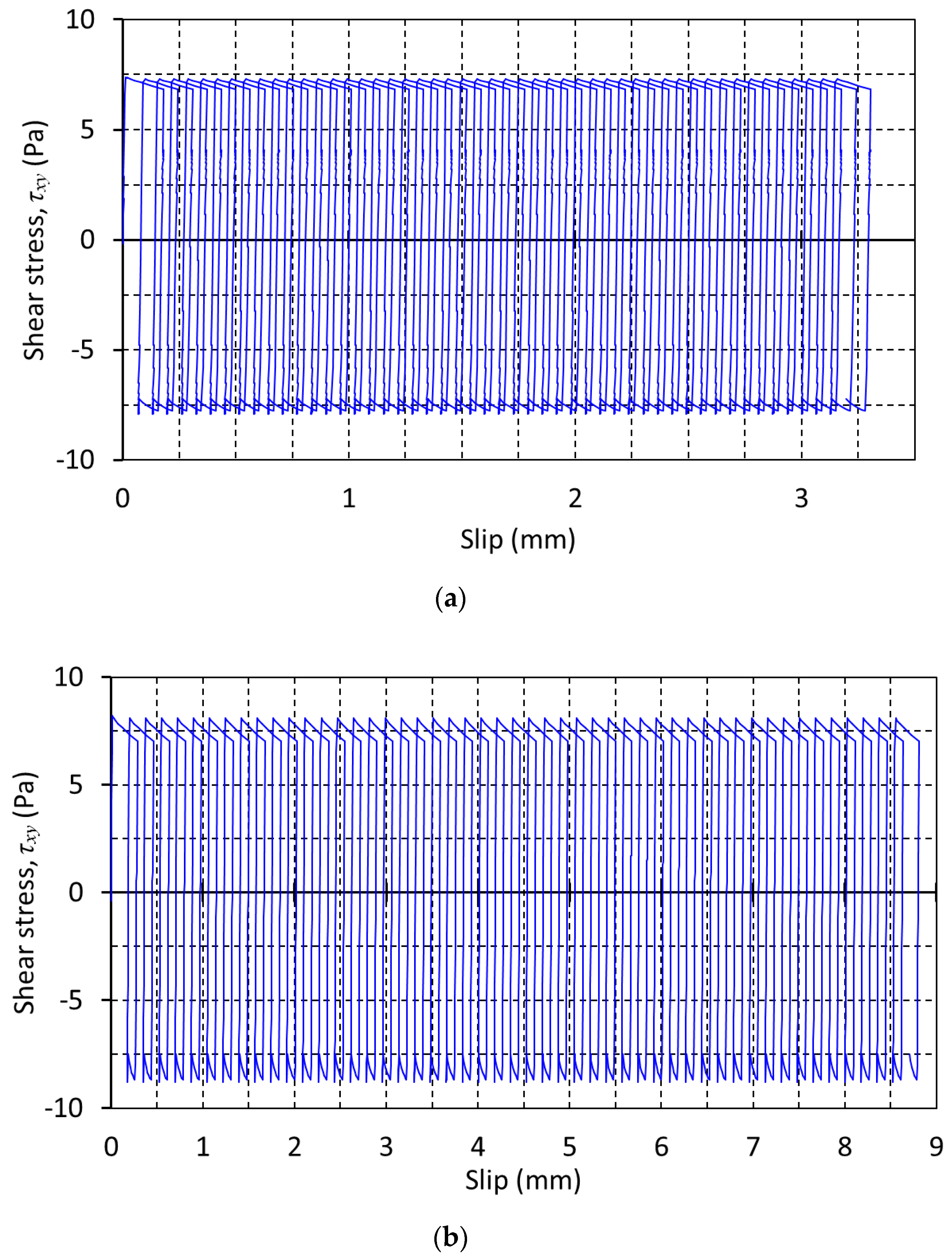
Lastly, Figure 15 describes the stress–slip relations during the repetitive heating–cooling cycles. The magnitude of the interface slip continuously grows while the interface shear stress alternates only within the same maximum and minimum values. That is, with the same temperature fluctuations, the slip ratcheting would gradually occur and continue to accumulate during the temperature cycles.

4. Numerical Study—Parametric Study

As revealed in the previous section, all these results—residual displacement, normal stresses, neutral point, and interface shear stress—are unique outcomes of each input parameter set. Therefore, the impact of individual input parameters on the presented model needs to be identified more; in this regard, we applied the seven different parameters—temperature amplitude ($\Delta T)$, elastic limit at the interface ($\delta )$, linear coefficient of thermal expansion ($\alpha )$, slope angle ($\beta )$, coefficient of friction ($\mu )$, density of the sliding material ($\rho )$, and Young’s modulus ($E)$—from the base case. The base case is the set of parameters in Table 1 with $\Delta T=23 °\mathrm{C}$ and $\beta =5°$ slope ($\delta =0.01 \mathrm{mm}$, $\alpha =7\times {10}^{-5}{ \mathrm{K}}^{-1}$, $\mu =0.271,$ $\rho =1.19 \mathrm{g}/{\mathrm{cm}}^3$, and $E=3.1 \mathrm{GPa}$). In this section, each one of these base case parameters is changed independently, and the corresponding results are compared. For example, three different temperature amplitudes, $\Delta T=23 °\mathrm{C}$, $31 °\mathrm{C}$, and $39 °\mathrm{C}$, are examined as shown in Figure 16a. The base case is marked with a thick solid line, and the other two are drawn with thin solid lines. Experimental test results observed in Figure 2 are also presented as a series of markers for comparisons.

As a result of simulations, the magnitude of accumulated slip increases with the higher values of $\Delta T$, $\alpha$, and $\beta$, and the lower value of $\mu$. On the other hand, other parameters, including $\delta$, $\rho$, and $E$, make a lesser impact or insignificant influence on the accumulated slip values. This observation agrees well with the landslide stability formula from geotechnical engineering [15], where the factor of safety for cohesionless soils is independent of the soil density.

The parametric study also shows the possible range of the residual slip accumulation after 50 temperature cycles. It can be inferred that the magnitude can be as small as $<1 \mathrm{mm}$ with a certain combination of the input parameters, but on the other hand, the magnitude could be possibly larger than $10 \mathrm{mm}$ in 50 cycles. Understanding that the slip value will only increase and never decrease, with a much larger number of temperature cycles, the slip can be piled up to the level with which the structural stability is critically hampered.

5. Discussion

As many computational works do, the presented model has some approximations implemented for the numerical study. Even though those approximations are not uncommon in many numerical studies and geotechnical engineering disciplines, the impact of those approximations is investigated here.

In this study, a two-dimensional (2D) plane strain numerical model is employed instead of a three-dimensional (3D) one, which would emulate the experimental condition better. In Figure 17, there is a certain difference between the 2D and 3D analyses, $3.213 \mathrm{mm}$ and $2.522 \mathrm{mm}$ after 50 temperature cycles, respectively. The discrepancy between these two approaches (approximately 21%) is not significantly large, considering the complexity of the slip ratcheting conditions. In fact, although running a 2D numerical model is neither dramatically faster nor easier, it is very typical to simplify a landslide problem into the 2D plane-strain condition in the discipline of geotechnical engineering ([15]). Furthermore, understanding the 2D model will surely be helpful to appreciate the 3D model. Particularly in this study, the 2D analysis has a great advantage over the 3D analysis because we aim to develop a theoretical approach for solving the slip ratcheting problem analytically in the following study.

Another approximation made in the numerical model is how the heating is applied to the acryl plate. In the experiments, the top of the acryl plate is heated by the heating pad attached to it. Then, the entire acryl plate is heated by the heat conduction, resulting in a temperature gradient in the transverse direction. On the other hand, the temperature of the entire acryl plate is increased at the same rate in the numerical model (that is, no temperature gradient). Hence, simulations in which a heat source is imposed at the top surface would rather reflect heat flux, and thus the transient temperature change in the acryl better. Simulations with such a setting were also conducted, and we compared the results in both 2D and 3D conditions; temperature inputs at the bottom of the acryl plate over the heating–cooling cycle are described in Figure 18a. There are no significant differences between the cases of experimentally measured one, simulation with constant temperature change, and simulation with transient temperature change. The residual slip, on the other hand, show much less difference. The slip values are $0.074 \mathrm{mm}$ and $0.060 \mathrm{mm}$ from the 2D and 3D analyses with the constant temperature change and $0.077 \mathrm{mm}$ and $0.071 \mathrm{mm}$ for the 2D and 3D analyses with the transient temperature change. The direct experimental value is not available but can be estimated as $0.067 \mathrm{mm}$ based on the trend line (a dotted blue line) of experimental observation.

6. Conclusions

Experimental evidence of the thermally-induced slip ratcheting is provided in this study, using an acryl sheet placed on a mildly-inclined wood slope. As a result of temperature increase and decrease of the acryl sheet, without any further loading, the sheet is observed to slide down gradually and continually. This is a consistent result with the other experiment settings, i.e., different temperature amplitudes and inclination angles.

The numerical model and simulation are also attempted to reproduce the major findings of the experiments. From the simulation work, it is found that there exists a neutral point in the acryl plate, and its location differs between the heating and cooling cycle of the plate. The shift of the neutral point appears to be the major reason for the residual slip after the temperature increase and decrease cycle because all the stresses are incurred repeatedly the same between the identical upper and lower limits. Although the magnitude of the residual slip is insignificant with one cycle, it continues to accumulate with a large number of cycles and could be sufficiently large to affect the overall stability.

The parametric study with the presented numerical model is also carried out to identify which input parameters play a major role in magnifying the residual slip values. It turns out that the accumulated slip values amplify with the increase of temperature amplitude (∆T), the coefficient of linear thermal expansion (α), and slope angle (β), and with the decrease in the coefficient of friction (μ). However, the elastic limit at the interface (δ), the density of the sliding material (ρ), and Young’s modulus (E) make a lesser impact or insignificant changes on the accumulated slip values.

References

1. Bakun-Mazor, D.; Hatzor, Y.H.; Glaser, S.D.; Santamarina, J.C. Thermally vs. seismically induced block displacements in Masada rock slopes. Int. J.Rock Mech. Min. Sci. 2013, 61, 196–211. [Google Scholar] [CrossRef]
2. Kim, S.; Druszkowski, E.; Zhang, J.; Kim, S. Numerical study on thermally-induced displacement ratcheting of a thin rock slab. In Geo-Congress 2019: Geotechnical Materials, Modeling, and Testing; American Society of Civil Engineers: Reston, VA, USA, 2019; pp. 506–513. [Google Scholar] [CrossRef]
3. Meier, J.; Bock, H. Stability of a block resting on an inclined plane—A classical problem revisited. Int. J. Rock Mech. Min. Sci. 2014, 70, 407–417. [Google Scholar] [CrossRef]
4. Pastén, C.; Santamarina, J.C. Experimental and numerical modeling of thermally-induced ratcheting displacement of geomembranes on slopes. Geosynth. Int. 2014, 21, 334–341. [Google Scholar] [CrossRef]
5. Croll, J.G.A. Thermally induced pulsatile motion of solids. Proc. R. Soc. A 2009, 465, 791–807. [Google Scholar] [CrossRef]
6. Murphy, K.D.; McCartney, J.S.; Henry, K.S. Evaluation of thermo-mechanical and thermal behavior of full-scale energy foundations. Acta Geotech. 2015, 10, 179–195. [Google Scholar] [CrossRef]
7. Suryatriyastuti, M.E.; Mroueh, H.; Burlon, S. A load transfer approach for studying the cyclic behavior of thermos-active piles. Comput. Geotech. 2014, 55, 378–391. [Google Scholar] [CrossRef]
8. Moseley, H. Descent of a solid body on an inclined plane when subject to alternations in temperature. Proc. R. Soc. 1855, vii, 333–342. [Google Scholar]
9. Rowe, R.K. Long-term performance of contaminant barrier systems. Géotechnique 2005, 55, 631–678. [Google Scholar] [CrossRef]
10. Take, W.A.; Chappel, M.J.; Brachman, R.W.I.; Rowe, R.K. Quantifying geomembrane wrinkles using aerial photography and digital image processing. Geosynth. Int. 2007, 14, 219–227. [Google Scholar] [CrossRef] [Green Version]
11. Uchida, E.; Azumi, R.; Norikane, Y. Light-induced crawling of crystals on a glass surface. Nat. Commun. 2015, 6, 7310. [Google Scholar] [CrossRef] [PubMed]
12. Pastén, C.; Garcia, M.; Cortes, D.D. Physical and numerical modeling of the thermally induced wedging mechanism. Geotech. Letters 2015, 5, 186–190. [Google Scholar] [CrossRef]
13. Pastén, C.; Castillo, E.; Chong, S.H. Thermo-mechanical ratcheting in soil-structure interfaces. Acta Geotech. 2019. [Google Scholar] [CrossRef]
14. ASTM D3080/D3080M-11, Standard Test Method for Direct Shear Test of Soils Under Consolidated Drained Conditions; ASTM International: West Conshohocken, PA, USA, 2011.
15. Duncan, J.M.; Wright, S.G.; Brandon, T.L. Soil Strength and Slope Stability, 2nd ed.; John Wiley & Sons, Inc.: Hoboken, NJ, USA, 2014; 317p. [Google Scholar]
Figure 1. Experimental study of the thermally induced slip ratcheting. (a) Picture of the overall experimental setup, (b) schematic of the test design, (c) temperature fluctuation of the heating pad using a power supply and on-and-off switch, which results in the amplitudes of about 23   ° C and 31   ° C for 5 V and 6 V applied, respectively, and (d) an example of the slip ratcheting captured by the camera.
Infrastructures 06 00005 g001
Figure 2. Slip growth with the number of temperature cycles from the experimental study. Four different cases ( 5   V and 6   V of power supply with 5 ° and 10 ° of the inclination angles) are presented with two separate implementations for each case.
Infrastructures 06 00005 g002
Figure 3. Results of the direct shear test at the acryl-wood interface; (a) normalized shear stress versus shear displacement from the multiple direct shear tests under the various range of normal stresses (results shown here are for 10 kPa of normal stress as an example), and (b) conceptual idealization of the direct shear test result.
Infrastructures 06 00005 g003
Figure 4. Results of the direct shear test at the acryl-wood interface; (a) determination of the frictional coefficient ( μ ), and (b) elastic limits of the shear displacement ( δ ) under various normal stresses and their regression fitting.
Infrastructures 06 00005 g004
Figure 5. (a) Conceptual schematic of the numerical model and (b) definitions of the stress values around the acryl plate.
Infrastructures 06 00005 g005
Figure 6. Comparison of the experiment and the simulation results with Δ T = 23   ° C in β = 5 ° slope. (a) Temperature cycles during the actual experiments and the numerical simulations, and (b) slip accumulation of the acryl vs. temperature cycles.
Infrastructures 06 00005 g006
Figure 7. Comparison of experiments and simulations—solid lines are the residual traces of numerical results and all the discrete markers are the experimental results.
Infrastructures 06 00005 g007
Figure 8. Distributions of normal stress ( σ x x ) on the acryl plate. The presented results are based on Δ T = 23   ° C in β = 5 ° slope with the parameters in Table 1. (a) gravity only (dotted line) and after 1st heating (red solid line) and cooling (blue solid line) and (b) after 50th heating (red solid line with cross) and cooling (blue solid line with tick) in addition to (a).
Infrastructures 06 00005 g008
Figure 9. Distributions of normal stress ( σ y y ) on the acryl plate. The presented results are based on Δ T = 23   ° C in β = 5 ° slope with the parameters in Table 1. (a) and (b) are the same as in Figure 8.
Infrastructures 06 00005 g009
Figure 10. Distributions of interface shear stress ( τ x y ) at the acryl-wood interface. The presented results are based on Δ T = 23   ° C in β = 5 ° slope with the parameters in Table 1. (a) and (b) are the same as in Figure 8.
Infrastructures 06 00005 g010
Figure 11. Distributions of the interface slip. The presented results are based on Δ T = 23   ° C in β = 5 ° slope with the parameters in Table 1. (a) gravity only (dotted line), after 1st heating (red solid line), during 1st cooling (blue dashed line), and after 1st cooling (blue solid line), (b) after 10th heating (red solid line with cross) and cooling (blue solid line with tick) in addition to (a), and (c) after 50th heating (red solid line with cross) and cooling (blue solid line with tick) in addition to (a).
Infrastructures 06 00005 g011aInfrastructures 06 00005 g011b
Figure 12. Distributions of normal stress ( σ x x ) on the acryl plate. The presented results are based on Δ T = 31   ° C in β = 10 ° slope with the parameters in Table 1. (a) and (b) are the same as in Figure 8.
Infrastructures 06 00005 g012
Figure 13. Distributions of interface shear stress ( τ x y ) at the acryl-wood interface. The presented results are based on Δ T = 31   ° C in β = 10 ° slope with the parameters in Table 1. (a) and (b) are the same as in Figure 8.
Infrastructures 06 00005 g013
Figure 14. Distributions of the interface slip. The presented results are based on Δ T = 31 ° C in β = 10 ° slope with the parameters in Table 1. (a), (b), and (c) are the same as in Figure 11.
Infrastructures 06 00005 g014
Figure 15. The slip build-up during the 50 temperature cycles. The presented results are based on the parameters in Table 1 with (a) Δ T = 23   ° C in β = 5 ° slope and (b) Δ T = 31   ° C in β = 10 ° slope.
Infrastructures 06 00005 g015
Figure 16. A parametric study with different inputs of temperature amplitude, elastic limit of the interface slip, and thermal expansion coefficient in (a), (b), and (c). The base case is set to Δ T = 23   ° C and β = 5 ° slope with the parameters in Table 1. Two experimental test results (1 and 2) for the base case are from Figure 2. A parametric study with different inputs of slope angle, friction coefficient, and acryl density in (d), (e), and (f). The base case is set to Δ T = 23   ° C and β = 5 ° slope with the parameters in Table 1. A parametric study with different inputs of Young’s modulus in (g). The base case is set to Δ T = 23   ° C and β = 5 ° slope with the parameters in Table 1.
Infrastructures 06 00005 g016aInfrastructures 06 00005 g016bInfrastructures 06 00005 g016c
Figure 17. Effect of the two-dimensional (2D) and 3D analyses on the residual slip vs. the number of temperature cycles.
Infrastructures 06 00005 g017
Figure 18. Effect of the transient heating condition on the residual slip. (a) Temperature change during the first heating–cooling cycle and (b) slip change.
Infrastructures 06 00005 g018