Towards More Sustainable Pavement Management Practices Using Embedded Sensor Technologies


Abstract
1. Introduction
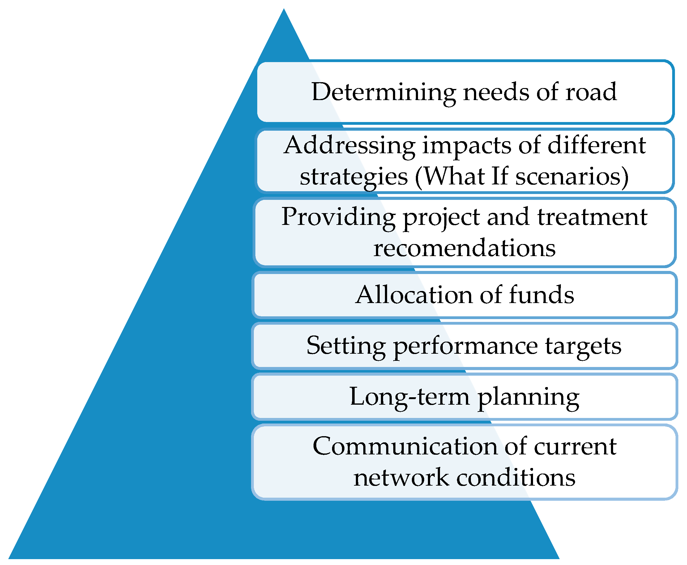
1.1. The Needs of Current Pavement Maintenance Systems and Practices
1.2. Environmental Concerns about Employing New Detection Systems
1.3. Aim of the Study
1.4. Structure of the Study
2. Embedded Sensors Considered in the Study
2.1. Strain Gauges
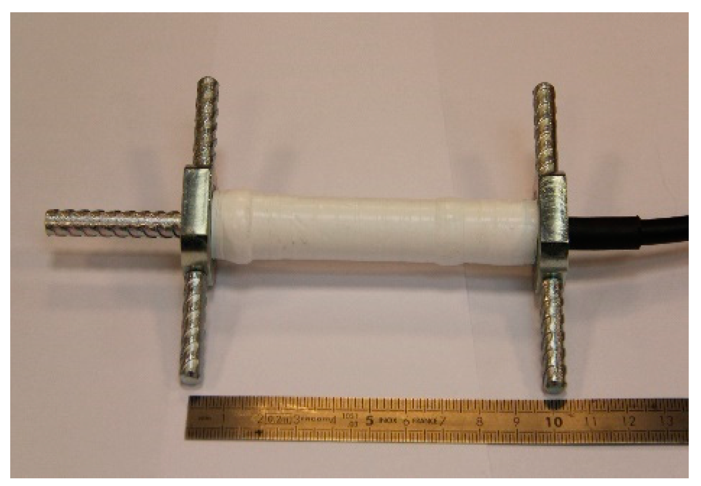
2.2. Piezoelectric Sensors
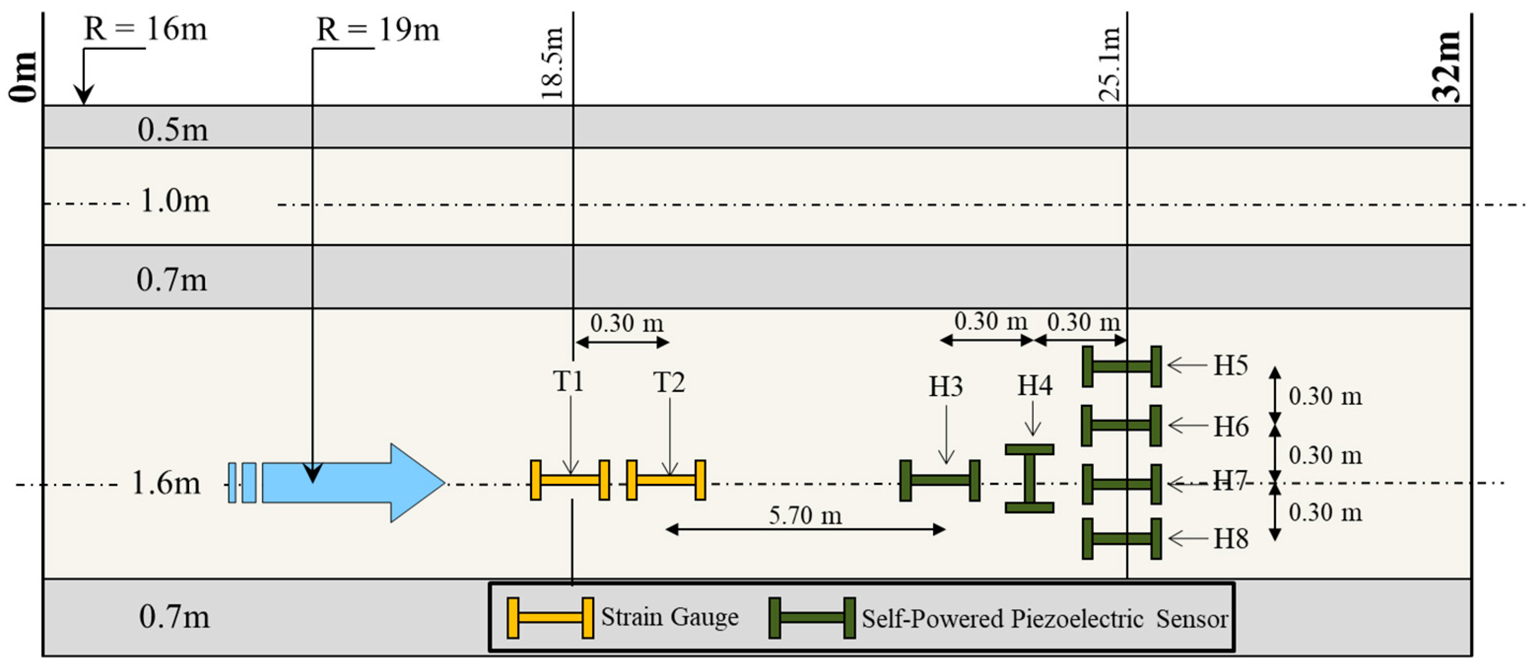
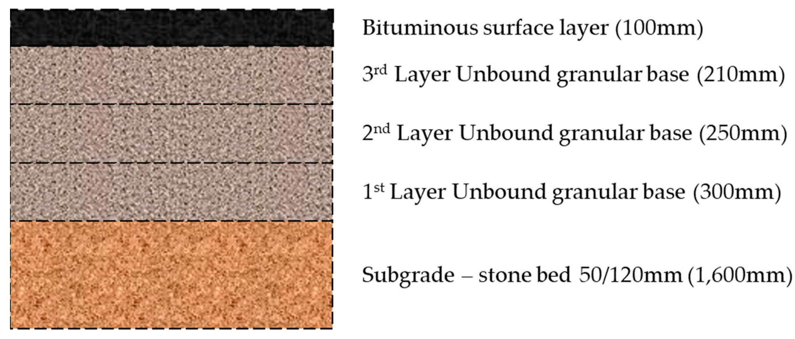
3. Experimental Test Section
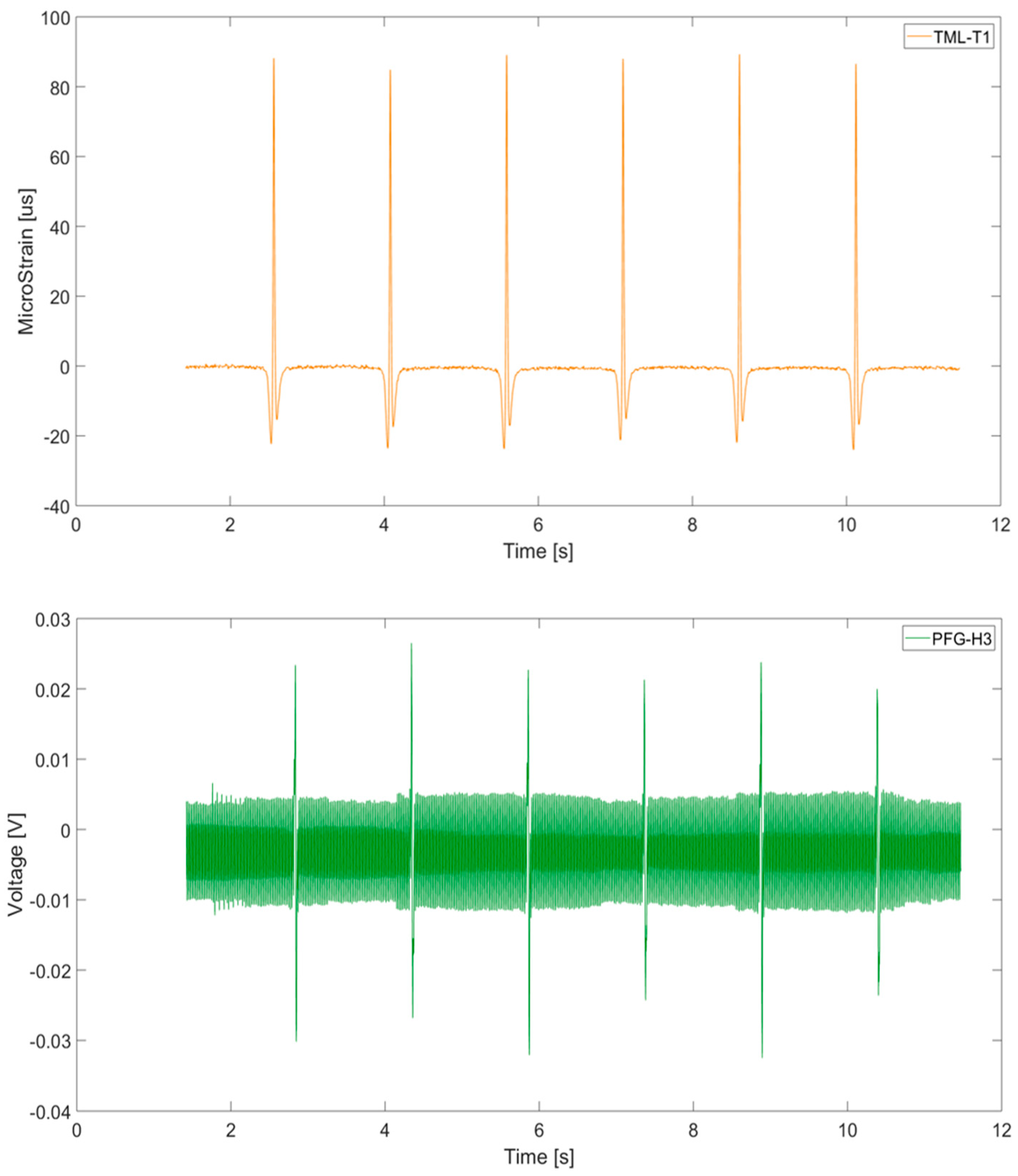
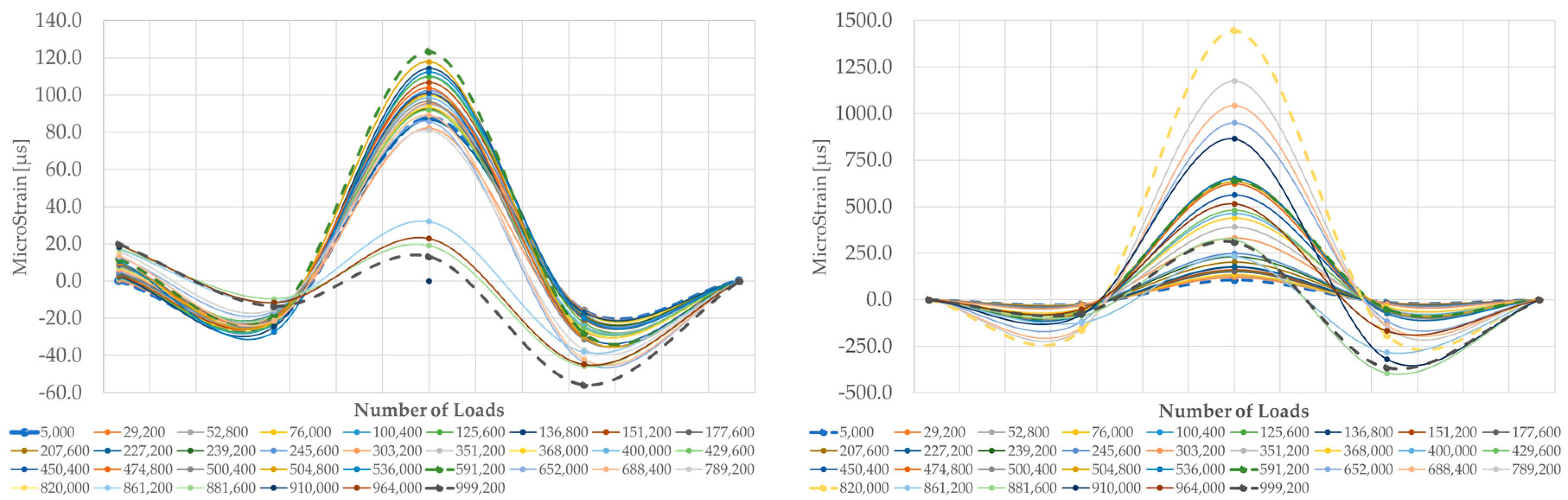
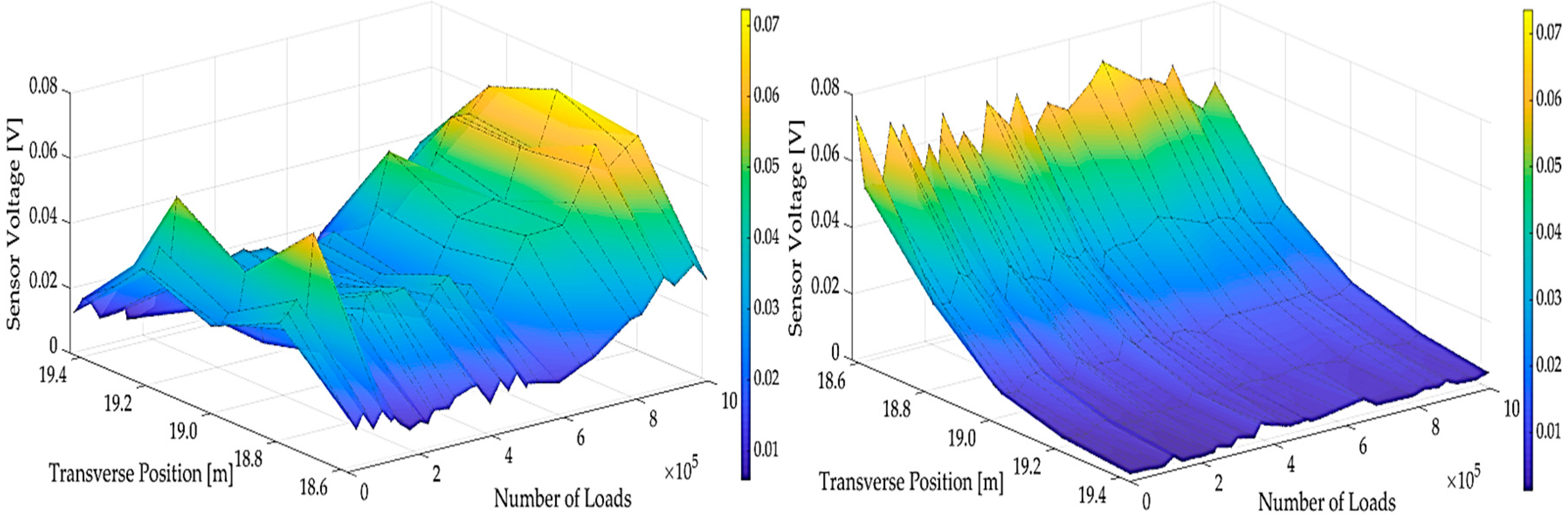
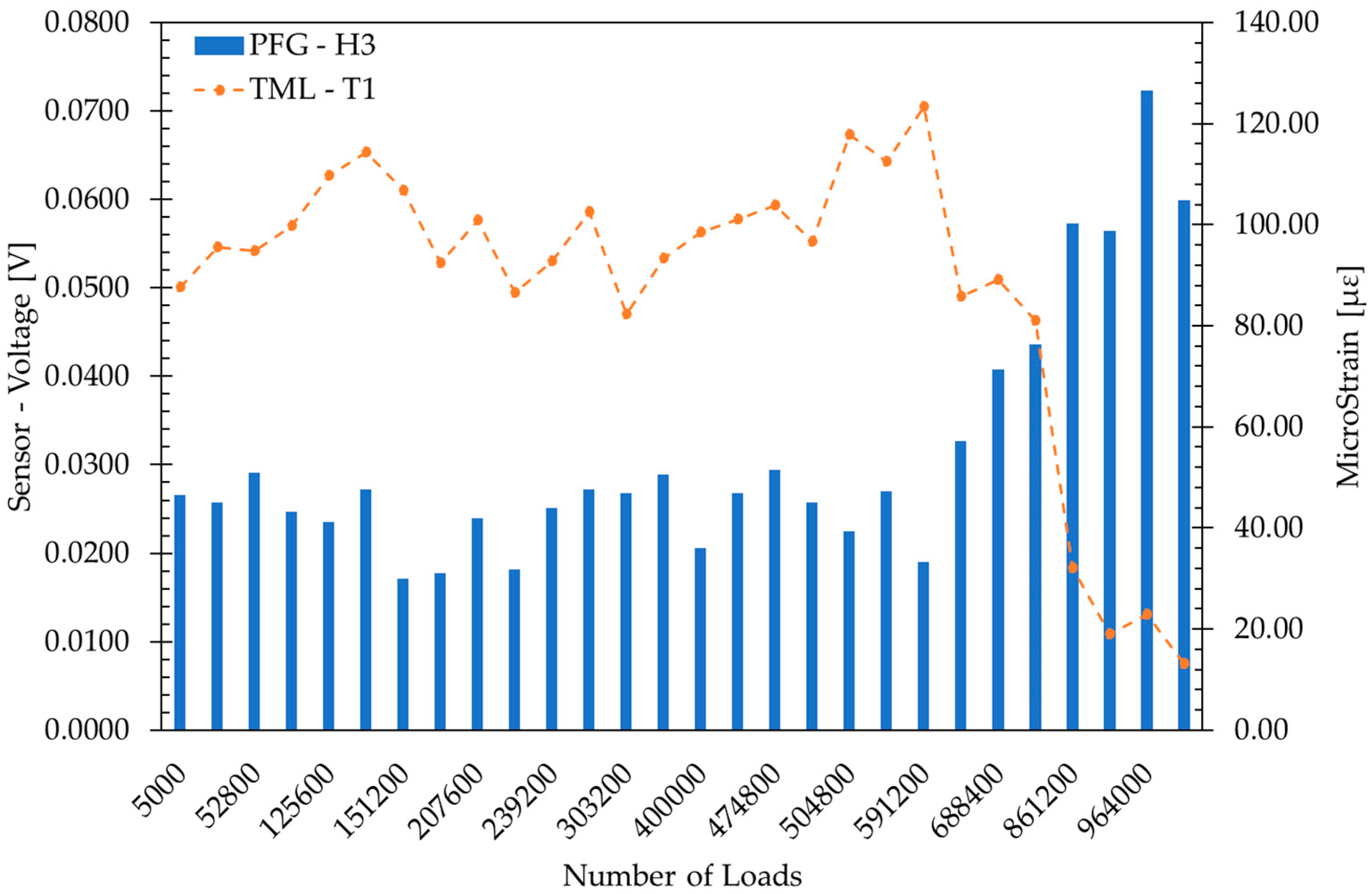
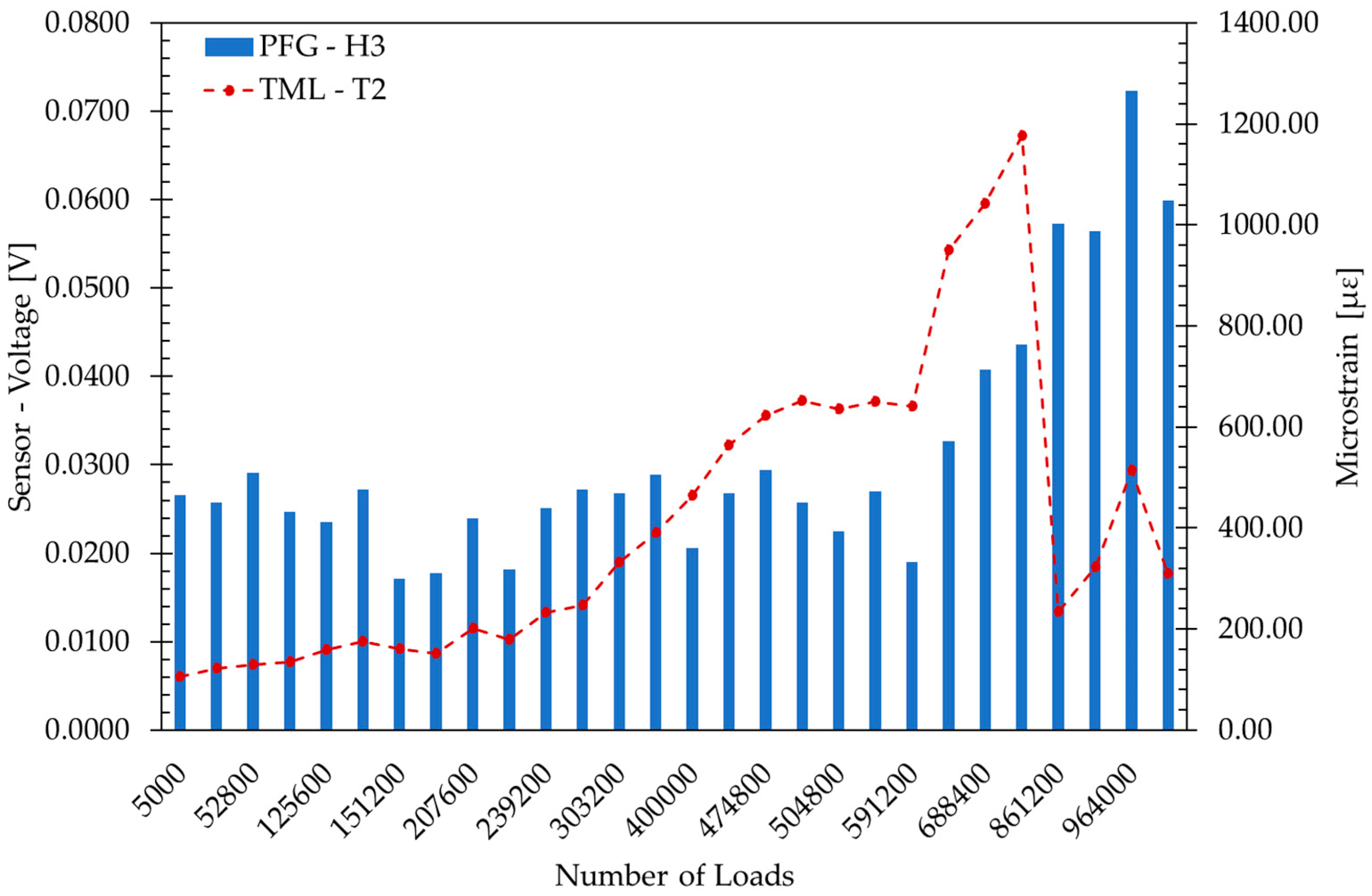
4. Sensor Results
5. Development of Maintenance Intervention Strategies
| 0: Do nothing | |
| 1: Cracks, rutting, potholes filling and sealing | [Routine Maintenance] |
| 2: Microsurfacing | [Routine Maintenance] |
| 3: Thin Overlay—2 cm Hot Mix Asphalt (HMA) | [Preventative Maintenance] |
| 4: Conventional structural mill and replace, Wearing course only | [Corrective Maintenance] |
| 5: Conventional structural mill and replace, wearing and binder | [Corrective Maintenance] |
5.1. Optimized Plan Based on PFG Sensors Response
5.2. Optimized Plan Based on Asphalt Strain Gauges Response
6. The Use of Life Cycle Assessment
6.1. Goal and Scope Definition
6.2. Functional Unit
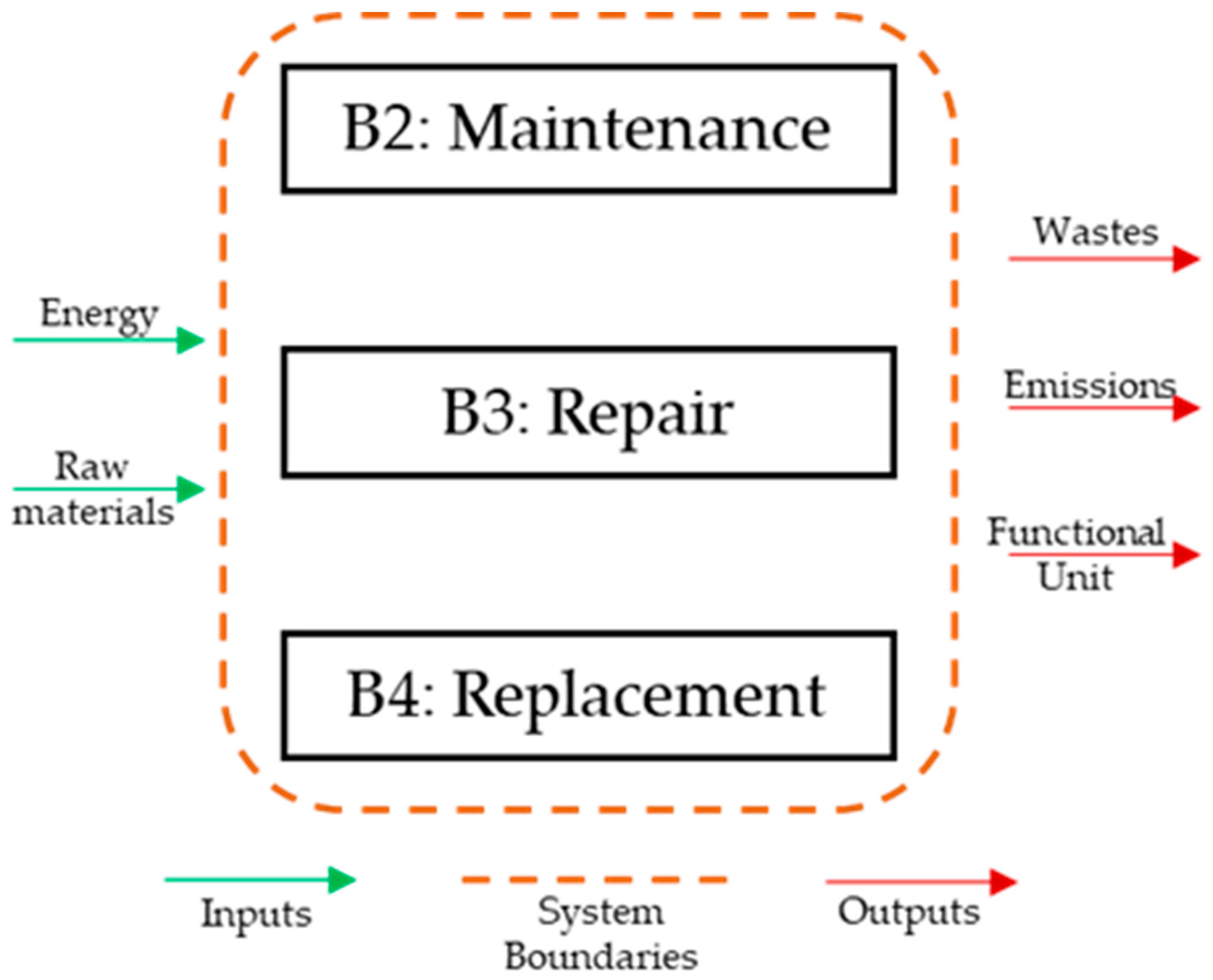
6.3. System Boundaries
6.4. Life Cycle Assessment Results
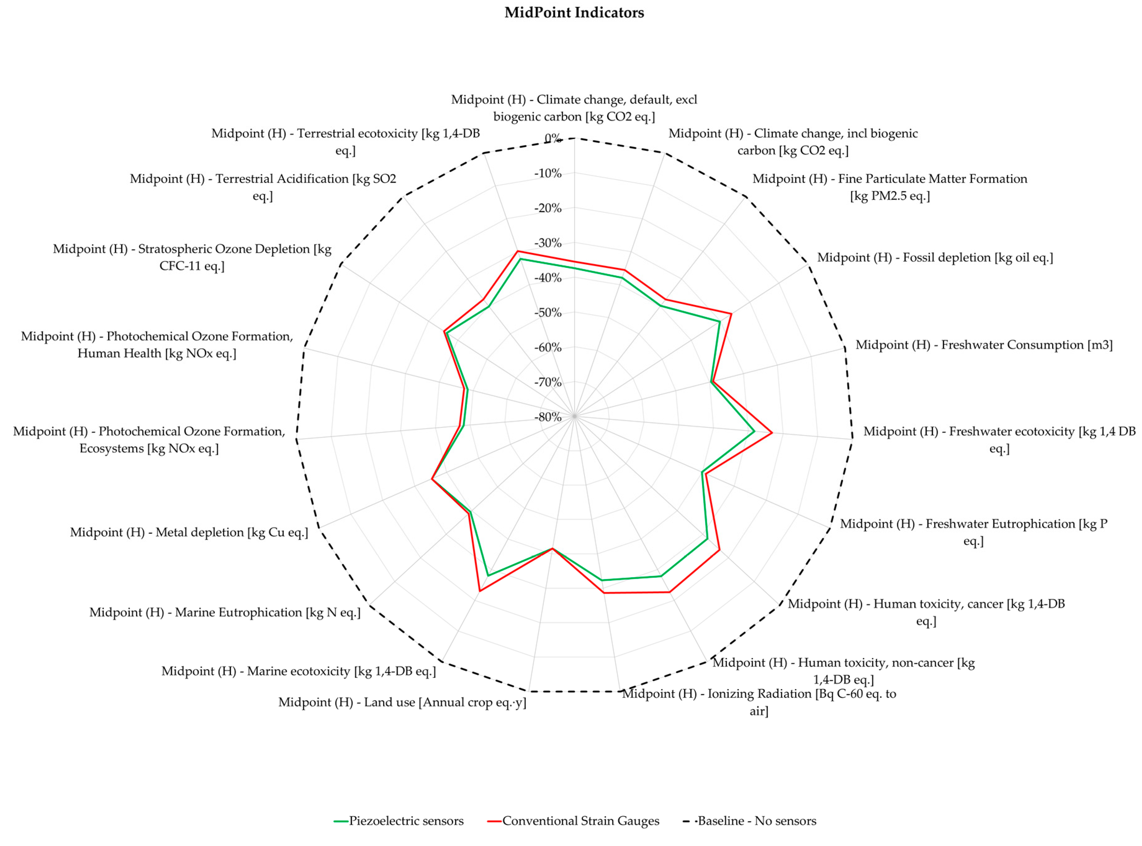
6.4.1. MidPoint Impact Category Indicators
6.4.2. EndPoint Impact Category Indicators
7. Summary and Conclusions
Author Contributions
Funding
Acknowledgments
Conflicts of Interest
References
- Vandam, T.J.; Harvey, J.T.; Muench, S.T.; Smith, K.D.; Snyder, M.B.; Al-Qadi, I.L.; Ozer, H.; Meijer, J.; Ram, P.V.; Roesier, J.R.; et al. Towards Sustainable Pavement Systems: A Reference Document FHWA-HIF-15-002; Federal Highway Administration: Washington, DC, USA, 2015. [Google Scholar]
- International Road Federation (IRF). IRF World Road Statistics 2018 (Data 2011–2016); International Road Federation (IRF): Brussels, Belgium, 2018. [Google Scholar]
- Peterson, D. National Cooperative Highway Research Program Synthesis of Highway Practice Pavement Management Practices. No. 135; Transportation Research Board: Washington, DC, USA, 1987; ISBN 0309044197. [Google Scholar]
- Li, X.; Goldberg, D.W. Toward a mobile crowdsensing system for road surface assessment. Comput. Environ. Urban Syst. 2018, 69, 51–62. [Google Scholar] [CrossRef]
- Radopoulou, S.C.; Brilakis, I. Improving Road Asset Condition Monitoring. Transp. Res. Procedia 2016, 14, 3004–3012. [Google Scholar] [CrossRef]
- Ragnoli, A.; De Blasiis, M.; Di Benedetto, A. Pavement Distress Detection Methods: A Review. Infrastructures 2018, 3, 58. [Google Scholar] [CrossRef]
- Coenen, T.B.J.; Golroo, A. A review on automated pavement distress detection methods. Cogent Eng. 2017, 4, 1374822. [Google Scholar] [CrossRef]
- Inzerillo, L.; Di Mino, G.; Roberts, R. Image-based 3D reconstruction using traditional and UAV datasets for analysis of road pavement distress. Autom. Constr. 2018, 96, 457–469. [Google Scholar] [CrossRef]
- Xue, W.; Wang, D.; Wang, L. A review and perspective about pavement monitoring. Int. J. Pavement Res. Technol. 2012, 5, 295–302. [Google Scholar]
- Lajnef, N.; Rhimi, M.; Chatti, K.; Mhamdi, L.; Faridazar, F. Toward an integrated smart sensing system and data interpretation techniques for pavement fatigue monitoring. Comput. Civ. Infrastruct. Eng. 2011, 26, 513–523. [Google Scholar] [CrossRef]
- Merenda, M.; Praticò, F.G.; Fedele, R.; Carotenuto, R.; Corte, F.G. Della A real-time decision platform for the management of structures and infrastructures. Electronics 2019, 8, 1180. [Google Scholar] [CrossRef]
- Fedele, R.; Praticò, F.G.; Carotenuto, R.; Della Corte, F.G. Energy savings in transportation: Setting up an innovative SHM method. Math. Model. Eng. Probl. 2018, 5, 323–330. [Google Scholar] [CrossRef]
- Hasni, H.; Alavi, A.H.; Chatti, K.; Lajnef, N. A self-powered surface sensing approach for detection of bottom-up cracking in asphalt concrete pavements: Theoretical/numerical modeling. Constr. Build. Mater. 2017, 144, 728–746. [Google Scholar] [CrossRef]
- American Association of State Highway and Transportation Officials (AASHTO). Pavement Management Guide; American Association of State Highway and Transportation Officials (AASHTO): Washington, DC, USA, 2012. [Google Scholar]
- Xue, W.; Wang, L.; Wang, D.; Druta, C. Pavement Health Monitoring System Based on an Embedded Sensing Network. J. Mater. Civ. Eng. 2014, 26, 04014072. [Google Scholar] [CrossRef]
- Duong, N.S.; Blanc, J.; Hornych, P.; Bouveret, B.; Carroget, J.; Le feuvre, Y. Continuous strain monitoring of an instrumented pavement section. Int. J. Pavement Eng. 2018, 8436, 1435–1450. [Google Scholar] [CrossRef]
- Gaborit, P.; Sauzéat, C.; Di Benedetto, H.; Pouget, S.; Olard, F.; Claude, A.; Monnet, A.J.; Audin, R.M.; Sauzéat, C.; Di Benedetto, H.; et al. Investigation of highway pavements using in-situ strain sensors. Int. Conf. Transp. Infrastruct. 2013, 28, 331. [Google Scholar]
- Blanc, J.; Hornych, P.; Duong, N.S.; Blanchard, J.Y.; Nicollet, P. Monitoring of an experimental motorway section. Road Mater. Pavement Des. 2017, 20, 74–89. [Google Scholar] [CrossRef]
- Stripple, H. Life Cycle Assessment of Road, A Pilot Study for Inventory Analysis; IVL RAPPORT. 1210; IVL: Linköping, Sweden, 2001; Volume 2. [Google Scholar]
- Carlson, A. Life Cycle Assessment of Roads and Pavements—Studies Made in Europe; VTI Rapp. 736A; Statens väg-och transportforskningsinstitut: Linköping, Sweden, 2011; Volume 22. [Google Scholar]
- ECRPD. Energy Conservation in Road Pavement Design, Maintenance and Utilisation. 2010, pp. 1–63. Available online: https://ec.europa.eu/energy/intelligent/projects/sites/iee-projects/files/projects/documents/ecrpd_publishable_report_en.pdf (accessed on 29 December 2019).
- The International Standards Organisation. Environmental Management—Life Cycle Assessment—Requirements and Guidelines; ISO 14044; The International Standards Organisation: Geneva, Switzerland, 2006; pp. 652–668. [Google Scholar]
- International Organization for Standardization. ISO 14040-Environmental Management—Life Cycle Assessment—Principles and Framework; The International Standards Organisation: Geneva, Switzerland, 2006; Volume 3, p. 20. [Google Scholar]
- Chappat, M.; Bilal, J. La route écologique du futur—Analyse du Cycle de Vie, Consommation d’énergie & émission de gaz à effet de serre. Développement Durable 2003, 40. [Google Scholar]
- Häkkinen, T.; Mäkelä, K. Environmental Impact of Concrete and Asphalt Pavements; Technical Research Center of Finland: Espoo, Finland, 1996; ISBN 9513849074. [Google Scholar]
- Mroueh, U.M.; Laine-Ylijoki, J.; Eskola, P. Life-cycle impacts of the use of industrial by-products in road and earth construction. Waste Manag. Ser. 2000, 1, 438–448. [Google Scholar]
- Hoang, T.; Jullien, A.; Ventura, A.; Crozet, Y. A global methodology for sustainable road—Application to the environmental assessment of French highway. In Proceedings of the 10 DBMC International Conference On Durability of Building Materials and Components, Lyon, France, 17–20 April 2005. [Google Scholar]
- Tokyo Measuring Instruments Lab. TML Pam E-2020C Tranducers 2017. Available online: https://tml.jp/eng/documents/Catalog/Transducers_E2020C.pdf (accessed on 12 November 2019).
- Karim, C.; Alavi, A..; Hassene, H.; Lajnef, N.; Faridazar, F. Damage Detection in Pavement Structures Using Self-powered Sensors. In Proceedings of the 8th RILEM International Conference on Mechanisms of Cracking and Debonding in Pavements, Nantes, France, 6–9 June 2016; Springer: Berlin, Germany, 2016; pp. 665–671. [Google Scholar]
- Lajnef, N.; Chatti, K.; Chakrabartty, S.; Rhimi, M.; Sarkar, P. Smart Pavement Monitoring System; Federal Highway Administration: Washington, DC, USA, 2013. [Google Scholar]
- Alavi, A.H.; Hasni, H.; Lajnef, N.; Chatti, K.; Faridazar, F. An intelligent structural damage detection approach based on self-powered wireless sensor data. Autom. Constr. 2016, 62, 24–44. [Google Scholar] [CrossRef]
- Loboratoire Central des Ponts et Chaussées. French Design Manual for Pavement Structures; Loboratoire Central des Ponts et Chaussées: Paris, France, 1997. [Google Scholar]
- SETRA-LCPC. Catalogue des Structures Types de chaussées Neuves; SETRA-LCPC: Paris, France, 1998. [Google Scholar]
- Laurent, G. Evaluation économique des chaussées en béton et classiques sur le réseau routier national français; ETUDES ET RECHERCHES DES LABORATOIRES DES PONTS ET CHAUSSEES-SERIE: ROUTES CR 33; ETUDES ET RECHERCHES DES LABORATOIRES DES PONTS ET CHAUSSEES: Paris, France, 2004. [Google Scholar]
- Mantalovas, K.; Di Mino, G. The sustainability of reclaimed asphalt as a resource for road pavement management through a circular economic model. Sustainbility 2019, 11, 2234. [Google Scholar] [CrossRef]
- Petho, L.; Denneman, E. Implementing EME2, the French high modulus asphalt in Australia. In Proceedings of the 6th Eurasphalt & Eurobitume Congress, Prague, Czech Republic, 1–3 June 2016. [Google Scholar]
- EAPA. Guidance Document for Preparing Product Category Rules (Pcr) and Environmental Product Declarations (Epd) for Asphalt Mixtures; EAPA: Arlington County, VA, USA, 2017; p. 43. [Google Scholar]
- Thinkstep AG Gabi ts 2019. Available online: https://www.thinkstep.com/content/gabi-databases-2019-edition (accessed on 29 December 2019).
- The Norwegian EPD Foundation. Product-Category Rules (PCR) for Preparing an Environmental Product Declaration (EPD) for Product Group Asphalt and Crushed Stone; The Norwegian EPD Foundation: Skien, Norway, 2009. [Google Scholar]
- EAPA. The Use of Warm Mix Asphalt; EAPA—Position paper; EAPA: Arlington County, VA, USA, 2014; p. 23. [Google Scholar]
- BRE. Product Category Rules for Type III Environmental Product Declaration of Construction Products to EN 15804:2012; BRE Group: Watford, UK, 2013; p. 43. [Google Scholar]
- European Bitumen Association. Life Cycle Inventory: Bitumen; European Bitumen Association: Harrogate, UK, 2012; ISBN 2930160268. [Google Scholar]
- EC-European Commission. COMMISSION RECOMMENDATION of 9 April 2013 on the Use of Common Methods to Measure and Communicate the Life Cycle Environmental Performance; EC-European Commission: Brussels, Belgium, 2013; pp. 1–45. [Google Scholar]
- Huijbregts, M.A.J.; Steinmann, Z.J.N.; Elshout, P.M.F.; Stam, G.; Verones, F.; Vieira, M.D.M.; Zijp, M.; van Zelm, R. ReCiPe 2016: A harmonized life cycle impact assessment method at midpoint and enpoint level—Report 1: Characterization. Natl. Inst. Public Health Environ. 2017, 22, 138–147. [Google Scholar]


| Load Applications | TML–T1 | TML–T2 | ||||
|---|---|---|---|---|---|---|
| Min-1 | Max | Min-2 | Min-1 | Max | Min-2 | |
| 5000 | −22.7 | 87.7 | −16.2 | −21.6 | 105.5 | −13.3 |
| 591,200 | −18.6 | 123.3 | −28.2 | −64.8 | 641.6 | −49.6 |
| 820,000 | N/A | N/A | N/A | −161.9 | 1446.7 | −190.2 |
| 999,200 | −13.5 | 13.2 | −55.8 | −72.1 | 309.4 | −364.8 |
| Year | 0 | 1 | 2 | 3 | 4 | 5 | 6 | 7 | 8 | 9 | 10 | 11 | 12 | 13 | 14 | 15 | 16 | 17 | 18 | 19 | 20 | 21 | 22 | 23 | 24 | 25 | 26 | 27 | 28 | 29 | 30 |
|---|---|---|---|---|---|---|---|---|---|---|---|---|---|---|---|---|---|---|---|---|---|---|---|---|---|---|---|---|---|---|---|
| Baseline Interventions | 0 | 0 | 0 | 0 | 0 | 0 | 0 | 0 | 1,2 | 0 | 0 | 0 | 0 | 0 | 0 | 4 | 0 | 0 | 0 | 0 | 0 | 0 | 0 | 1,2 | 0 | 0 | 0 | 0 | 0 | 0 | 5 |
| Threshold | H3 | H7 | ||
|---|---|---|---|---|
| Definition | Activation | Definition | Activation | |
| 1 | 0.018 | -- | 0.016 | -- |
| 2 | 0.025 | -- | 0.028 | -- |
| 3 | 0.031 | 591,200 | 0.038 | 125,600 |
| 4 | 0.038 | 591,200 | 0.048 | 125,600 |
| 5 | 0.045 | 789,200 | 0.059 | N/A |
| 6 | 0.051 | 789,200 | 0.069 | N/A |
| 7 | 0.058 | 789,200 | 0.080 | N/A |
| Year | 0 | 1 | 2 | 3 | 4 | 5 | 6 | 7 | 8 | 9 | 10 | 11 | 12 | 13 | 14 | 15 | 16 | 17 | 18 | 19 | 20 | 21 | 22 | 23 | 24 | 25 | 26 | 27 | 28 | 29 | 30 |
|---|---|---|---|---|---|---|---|---|---|---|---|---|---|---|---|---|---|---|---|---|---|---|---|---|---|---|---|---|---|---|---|
| Optimized Interventions | 0 | 0 | 0 | 0 | 0 | 1 | 0 | 0 | 0 | 2 | 0 | 0 | 0 | 1,3 | 0 | 0 | 0 | 0 | 0 | 1 | 0 | 0 | 0 | 4 | 0 | 0 | 0 | 0 | 0 | 0 | 1,3 |
| Year | 0 | 1 | 2 | 3 | 4 | 5 | 6 | 7 | 8 | 9 | 10 | 11 | 12 | 13 | 14 | 15 | 16 | 17 | 18 | 19 | 20 | 21 | 22 | 23 | 24 | 25 | 26 | 27 | 28 | 29 | 30 | |
|---|---|---|---|---|---|---|---|---|---|---|---|---|---|---|---|---|---|---|---|---|---|---|---|---|---|---|---|---|---|---|---|---|
| Optimized Interventions | 0 | 0 | 0 | 0 | 0 | 0 | 1 | 0 | 0 | 0 | 2 | 1 | 0 | 0 | 0 | 1,3 | 0 | 0 | 0 | 0 | 1 | 0 | 0 | 0 | 4 | 0 | 0 | 0 | 0 | 0 | 1,3 |
© 2019 by the authors. Licensee MDPI, Basel, Switzerland. This article is an open access article distributed under the terms and conditions of the Creative Commons Attribution (CC BY) license (http://creativecommons.org/licenses/by/4.0/).
Share and Cite
Manosalvas-Paredes, M.; Roberts, R.; Barriera, M.; Mantalovas, K. Towards More Sustainable Pavement Management Practices Using Embedded Sensor Technologies. Infrastructures 2020, 5, 4. https://doi.org/10.3390/infrastructures5010004
Manosalvas-Paredes M, Roberts R, Barriera M, Mantalovas K. Towards More Sustainable Pavement Management Practices Using Embedded Sensor Technologies. Infrastructures. 2020; 5(1):4. https://doi.org/10.3390/infrastructures5010004
Chicago/Turabian StyleManosalvas-Paredes, Mario, Ronald Roberts, Maria Barriera, and Konstantinos Mantalovas. 2020. "Towards More Sustainable Pavement Management Practices Using Embedded Sensor Technologies" Infrastructures 5, no. 1: 4. https://doi.org/10.3390/infrastructures5010004
APA StyleManosalvas-Paredes, M., Roberts, R., Barriera, M., & Mantalovas, K. (2020). Towards More Sustainable Pavement Management Practices Using Embedded Sensor Technologies. Infrastructures, 5(1), 4. https://doi.org/10.3390/infrastructures5010004