Prediction of Compression Index of Fine-Grained Soils Using a Gene Expression Programming Model

 ,
, 
 ,
,
Abstract
:
1. Introduction
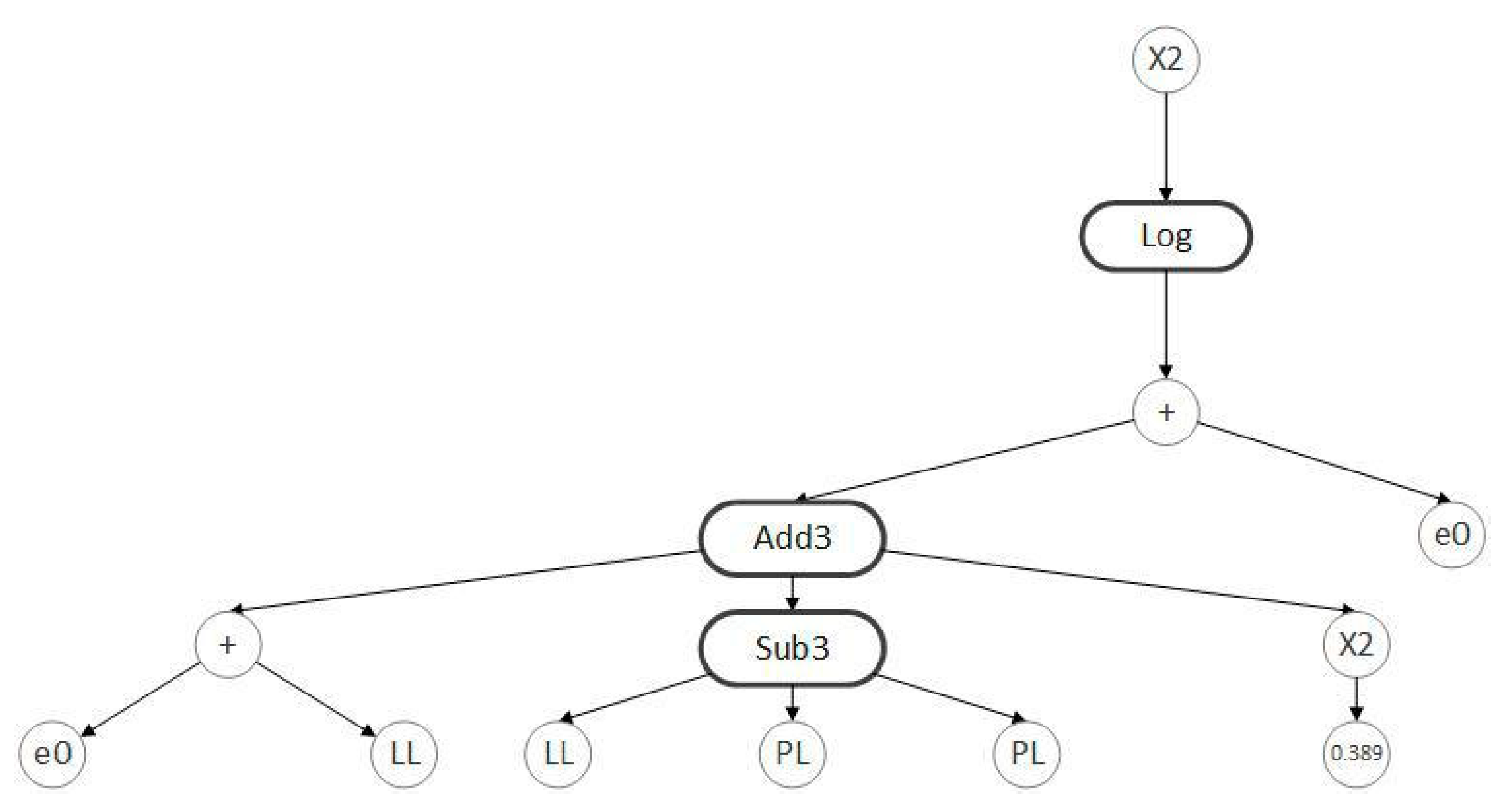
2. GEP
3. Modeling of Cc for Fine-Grained Soils
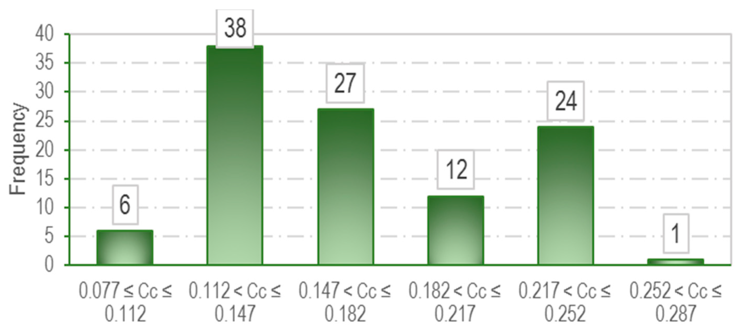
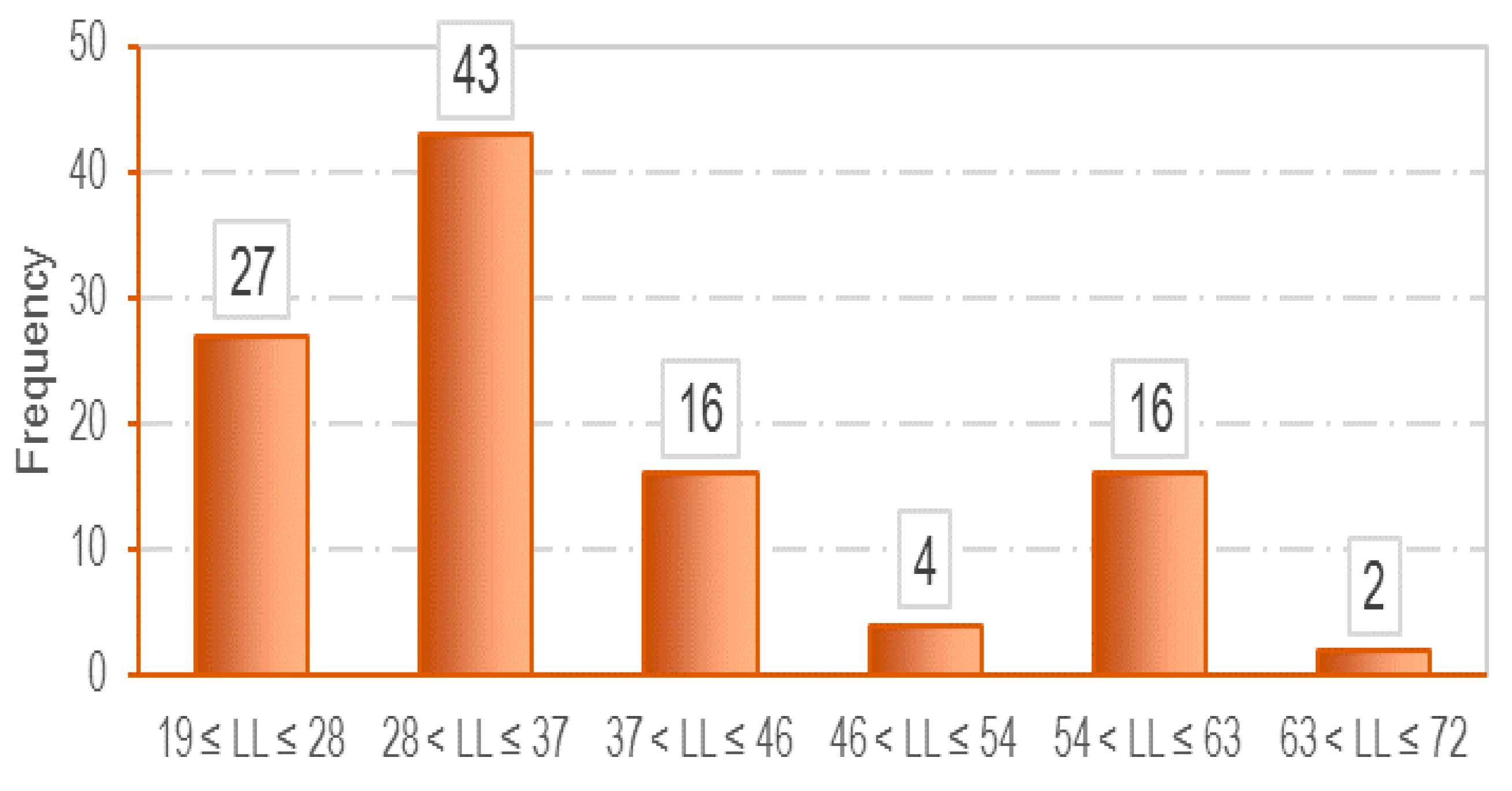
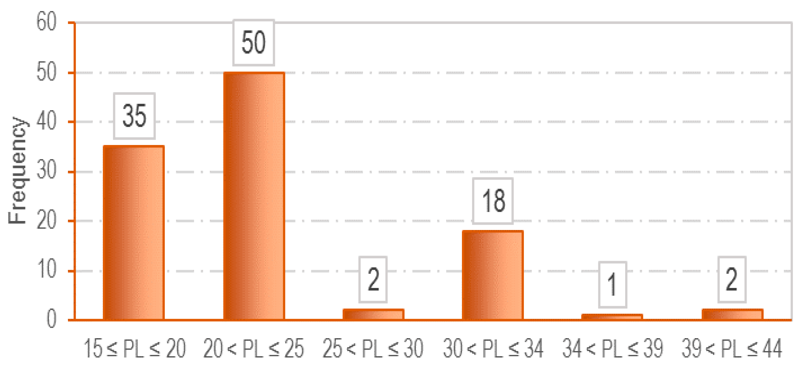
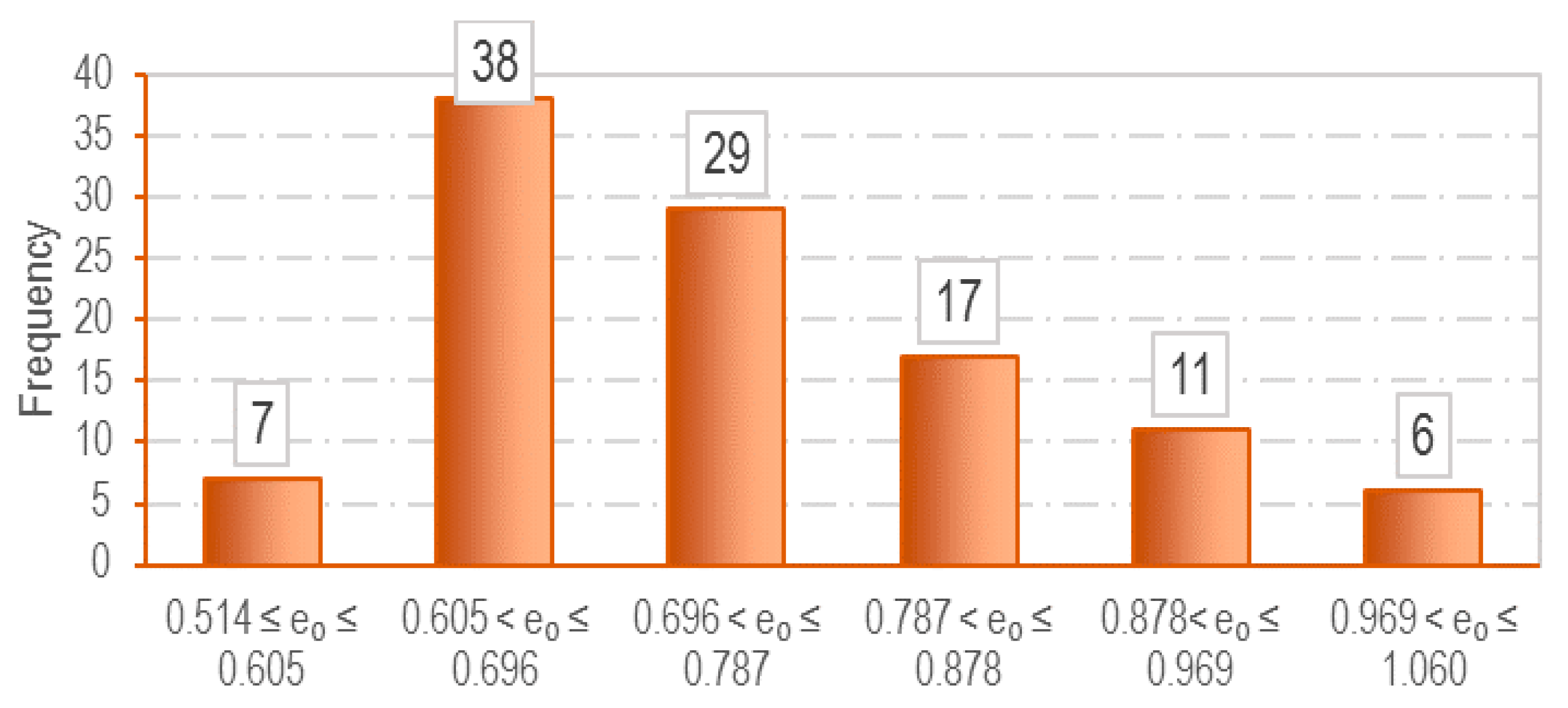
3.1. Data Collection
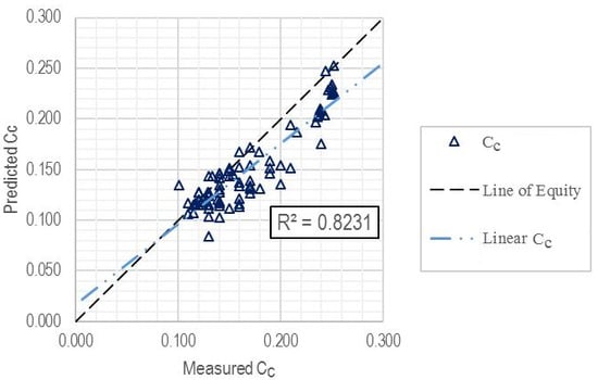
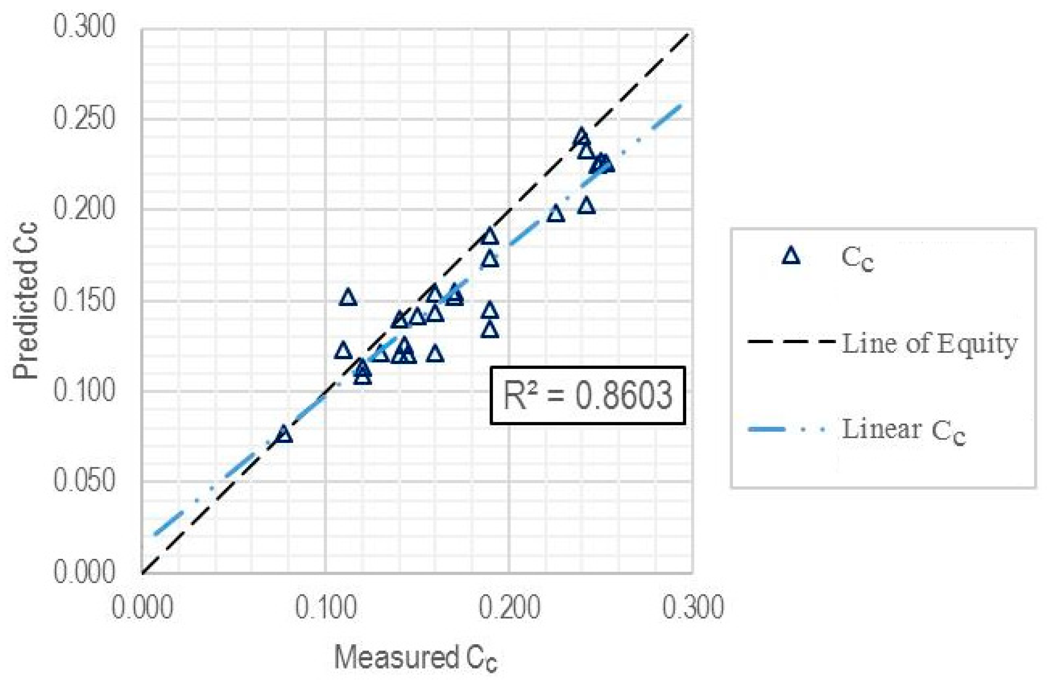
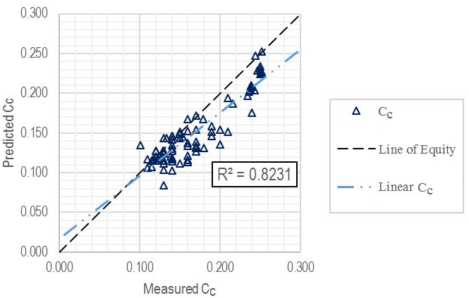
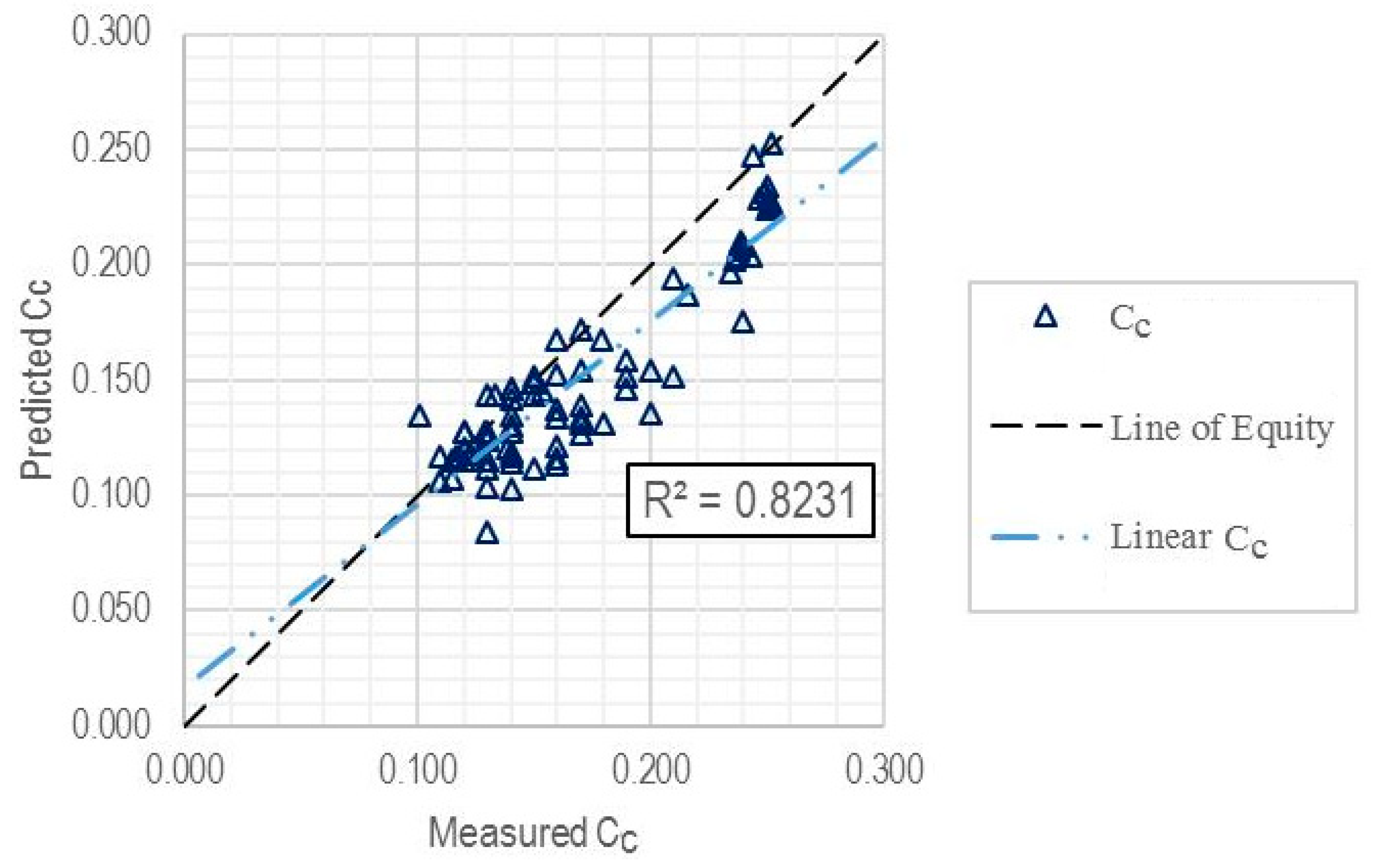
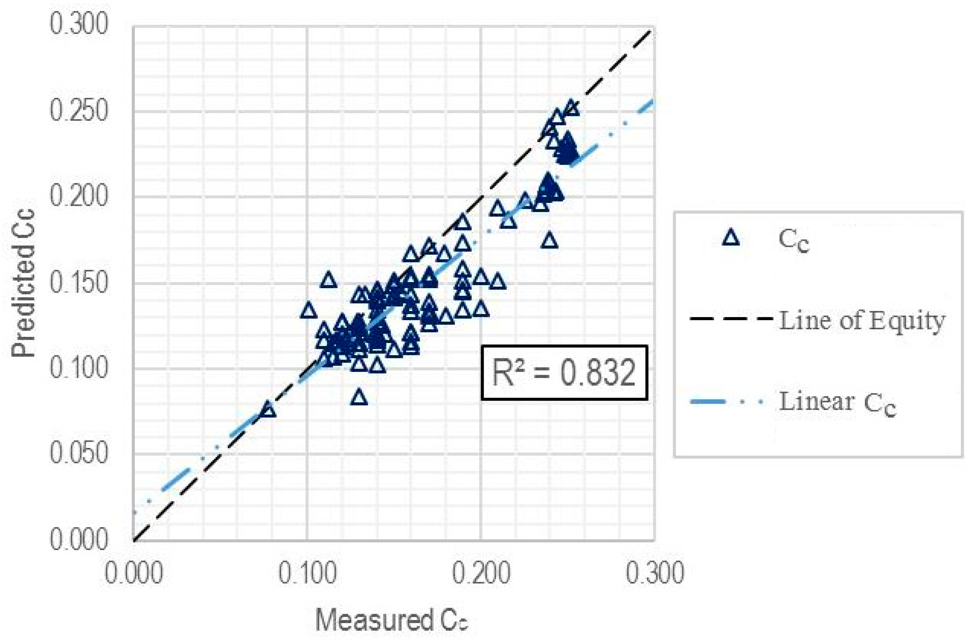
3.2. Model Structure and Performance
3.3. Model Development
3.4. Additional Evaluation of Model Performance
4. Conclusions
Author Contributions
Funding
Conflicts of Interest
References
- Tiwari, B.; Ajmera, B. New correlation equations for compression index of remolded clays. J. Geotech. Geoenviron. Eng. 2011, 138, 757–762. [Google Scholar] [CrossRef]
- Carter, M.; Bentley, S.P. Correlations of Soil Properties; Pentech Press Publishers: Philadelphia, NJ, USA, 1991. [Google Scholar]
- Azzouz, A.S.; Krizek, R.J.; Corotis, R.B. Regression analysis of soil compressibility. SOILS Found. 1976, 16, 19–29. [Google Scholar] [CrossRef]
- Cozzolino, V. Statistical forecasting of compression index. In Proceedings of the Fifth International Conference on Soil Mechanics and Foundation Engineering, Paris, France, 17–22 July 1961; pp. 51–53. [Google Scholar]
- Mayhe, P. Cam-clays predictions of undrained strength. J. Geotech. Geoenviron. Eng. 1980, 106, 1219–1242. [Google Scholar]
- Nishida, Y. A brief note on compression index of soil. J. Soil Mech. Found. Div. 1956, 82, 1–14. [Google Scholar]
- Park, H.I.; Lee, S.R. Evaluation of the compression index of soils using an artificial neural network. Comput. Geotech. 2011, 38, 472–481. [Google Scholar] [CrossRef]
- Skempton, A.W.; Jones, O.T.; Quennell, A.M. Notes on the compressibility of clays. Q. J. Geol. Soc. 1944, 100, 119–135. [Google Scholar] [CrossRef]
- Terzaghi, K.; Peck, R.B.; Mesri, G. Soil Mechanics in Engineering Practice; John Wiley & Sons: Dallas, TX, USA, 1996. [Google Scholar]
- Alavi, A.H.; Gandomi, A.H. A robust data mining approach for formulation of geotechnical engineering systems. Eng. Comput. 2011, 28, 242–274. [Google Scholar] [CrossRef]
- Choubin, B.; Moradi, E.; Golshan, M.; Adamowski, J.; Sajedi-Hosseini, F.; Mosavi, A. An ensemble prediction of flood susceptibility using multivariate discriminant analysis, classification and regression trees, and support vector machines. Sci. Total. Environ. 2019, 651, 2087–2096. [Google Scholar] [CrossRef]
- Rezakazemi, M.; Mosavi, A.; Shirazian, S. ANFIS pattern for molecular membranes separation optimization. J. Mol. Liq. 2019, 274, 470–476. [Google Scholar] [CrossRef]
- Mosavi, A.; Ozturk, P.; Chau, K.-W. Flood Prediction Using Machine Learning Models: Literature Review. Water 2018, 10, 1536. [Google Scholar] [CrossRef]
- Mosavi, A.; Lopez, A.; Varkonyi-Koczy, A.R. Industrial applications of big data: State of the art survey. In Proceedings of the International Conference on Global Research and Education, Lasi, Romania, 25–28 September 2017; pp. 225–232. [Google Scholar]
- Mosavi, A.; Bathla, Y.; Varkonyi-Koczy, A. Predicting the future using web knowledge: State of the art survey. In Proceedings of the International Conference on Global Research and Education, Lasi, Romania, 25–28 September 2017; pp. 341–349. [Google Scholar]
- Vargas, R.; Mosavi, A.; Ruiz, R. Deep learning: A review. Adv. Intell. Syst. Comput. 2017, 7, 122–148. [Google Scholar]
- Mosavi, A.; Rabczuk, T. Learning and intelligent optimization for material design innovation. In Proceedings of the International Conference on Learning and Intelligent Optimization, Russia, Novgorod, 19 June 2017; pp. 358–363. [Google Scholar]
- Mosavi, A.; Rabczuk, T.; Varkonyi-Koczy, A.R. Reviewing the novel machine learning tools for materials design. In Proceedings of the International Conference on Global Research and Education, Lasi, Romania, 23 September 2017; pp. 50–58. [Google Scholar]
- Mosavi, A.; Varkonyi-Koczy, A.R. Integration of machine learning and optimization for robot learning. In Recent Global Research and Education: Technological Challenges; Springer: Lasi, Romaria, 2017; pp. 349–355. [Google Scholar]
- Mosavi, A.; Edalatifar, M. A Hybrid Neuro-Fuzzy Algorithm for Prediction of Reference Evapotranspiration. In Proceedings of the International Conference on Global Research and Education, Kaunas, Lithuania, 4 September 2017; pp. 235–243. [Google Scholar]
- Torabi, M.; Mosavi, A.; Ozturk, P.; Varkonyi-Koczy, A.; Istvan, V. A hybrid machine learning approach for daily prediction of solar radiation. In Proceedings of the International Conference on Global Research and Education, Kaunas, Lithuania, 24–27 September 2018; pp. 266–274. [Google Scholar]
- Das, S.K.; Basudhar, P.K. Prediction of residual friction angle of clays using artificial neural network. Eng. Geol. 2008, 100, 142–145. [Google Scholar] [CrossRef]
- Das, S.K.; Biswal, R.K.; Sivakugan, N.; Das, B. Classification of slopes and prediction of factor of safety using differential evolution neural networks. Environ. Earth Sci. 2011, 64, 201–210. [Google Scholar] [CrossRef]
- Daryaei, M.; Kashefipour, S.M.; Ahadian, J.; Ghobadian, R. Modeling the compression index of fine soils using artificial neural network and comparison with the other empirical equations. J. Water Soil 2010, 5, 312–333. [Google Scholar]
- Farkhonde, S.; Bolouri, J. Estimation of compression index of clayey soils using artificial neural network. In Proceedings of the Fifth National Conference on Civil Engineering, Mashhad, Iran, 10 May 2018. [Google Scholar]
- Kumar, V.P.; Rani, C.S. Prediction of compression index of soils using artificial neural networks (ANNs). Int. J. Eng. Res. Appl. 2011, 1, 1554–1558. [Google Scholar]
- Talaei-Khoei, A.; Wilson, J.M.; Kazemi, S.-F. Period of Measurement in Time-Series Predictions of Disease Counts from 2007 to 2017 in Northern Nevada: Analytics Experiment. JMIR Public Health Surveill. 2019, 5, e11357. [Google Scholar] [CrossRef] [PubMed]
- Mohammadzadeh, D.; Bazaz, J.B.; Yazd, S.V.J.; Alavi, A.H. Deriving an intelligent model for soil compression index utilizing multi-gene genetic programming. Environ. Earth Sci. 2016, 75, 262. [Google Scholar] [CrossRef]
- Mohammadzadeh, D.; Bazaz, J.B.; Alavi, A.H. An evolutionary computational approach for formulation of compression index of fine-grained soils. Eng. Appl. Artif. Intell. 2014, 33, 58–68. [Google Scholar] [CrossRef]
- Kazemi, S.F.; Shafahi, Y. An Integrated Model Of Parallel Processing And PSO Algorithm For Solving Optimum Highway Alignment Problem. In Proceedings of the ECMS, Aesund, Norway, 12 June 2013; pp. 551–557. [Google Scholar]
- Ferreira, C. Gene Expression Programming: Mathematical Modeling by an Artificial Intelligence; Springer: Bristol, UK, 2006; Volume 21. [Google Scholar]
- Ferreira, C. Gene expression programming and the evolution of computer programs. In Recent Developments in Biologically Inspired Computing; Springer: Oxford, UK, 2004; pp. 82–103. [Google Scholar]
- Koza, J.R. Genetic Programming: on the Programming of Computers by Means of Natural Selection; MIT Press: London, UK, 1992; Volume 1. [Google Scholar]
- Ferreira, C. Gene expression programming in problem solving. In Soft Computing and Industry; Springer: Angra do Heroismo, Portugal, 2002; pp. 635–653. [Google Scholar]
- Batioja-Alvarez, D.D.; Kazemi, S.-F.; Hajj, E.Y.; Siddharthan, R.V.; Hand, A.J.T. Probabilistic Mechanistic-Based Pavement Damage Costs for Multitrip Overweight Vehicles. J. Transp. Eng. Part B Pavements 2018, 144, 04018004. [Google Scholar] [CrossRef]
- Standard Test Methods for Liquid Limit, Plastic Limit, and Plasticity Index of Soils; ASTM International: Washington, DC, USA, 2017.
- ASTM. Standard Test Method for Bulk Specific Gravity and Density of Non-Absorptive Compacted Asphalt Mixtures; ASTM International: Washington, DC, USA, 2017. [Google Scholar]
- Standard Test Methods for One-Dimensional Consolidation Properties of Soils Using Incremental Loading; ASTM International: Washington, DC, USA, 2011.
- Gandomi, A.H.; Mohammadzadeh, D.; Pérez-Ordóñez, J.L.; Alavi, A.H. Linear genetic programming for shear strength prediction of reinforced concrete beams without stirrups. Appl. Soft Comput. 2014, 19, 112–120. [Google Scholar] [CrossRef]
- Ziaee, S.A.; Sadrossadat, E.; Alavi, A.H.; Shadmehri, D.M. Explicit formulation of bearing capacity of shallow foundations on rock masses using artificial neural networks: Application and supplementary studies. Environ. Earth Sci. 2015, 73, 3417–3431. [Google Scholar] [CrossRef]
- Gepsoft GeneXproTools, version 5.0; Gepsoft: Bristol, UK, 2014.
- Smith, G.N. Probability and Statistics in Civil Engineering; Collins Professional and Technical Books; Collins: London, UK, 1986; 244p. [Google Scholar]
- Golbraikh, A.; Tropsha, A. Beware of q2! J. Mol. Graph. Model. 2002, 20, 269–276. [Google Scholar] [CrossRef]
- Roy, P.P.; Roy, K. On Some Aspects of Variable Selection for Partial Least Squares Regression Models. QSAR Comb. Sci. 2008, 27, 302–313. [Google Scholar] [CrossRef]


| Parameter | LL (%) | PL (%) | e0 | Cc |
|---|---|---|---|---|
| Mean | 36.16 | 22.61 | 0.75 | 0.17 |
| Standard Deviation | 12.79 | 5.64 | 0.12 | 0.05 |
| Minimum | 19.40 | 14.80 | 0.51 | 0.08 |
| Maximum | 72.00 | 44.00 | 1.03 | 0.025 |
| Range | 52.60 | 29.20 | 0.52 | 0.18 |
| Parameter | Setting |
|---|---|
| Number of chromosomes | 50 to 1000 |
| Number of genes | 3 |
| Head size | 8 |
| Tail size | 17 |
| Dc size | 17 |
| Gene size | 42 |
| Gene recombination rate | 0.277 |
| Gene transportation rate | 0.277 |
| Function set | +, −, ×, /, exp, ln, and Inv |
| Set | Number of Data Points | R2 | RMSE | MAE |
|---|---|---|---|---|
| Training subset | 81 | 0.8231 | 0.0269 | 0.0213 |
| Validation subset | 27 | 0.8603 | 0.0237 | 0.0189 |
| Entire dataset | 108 | 0.8320 | 0.0262 | 0.0207 |
| Statistical Parameter | Source | Criteria | Evaluation for GEP-Based Model |
|---|---|---|---|
| Golbraikh and Tropsha [43] | 0.85 < k < 1.15 | 1.001 | |
| Roy and Roy [44] | 0.85 < k’ < 1.15 | 0.989 | |
| Roy and Roy [44] | 0.5 < Rm | 0.503 | |
| Roy and Roy [44] | Should be close to 1.0 | 1.000 | |
| Roy and Roy [44] | Should be close to 1.0 | 0.998 |
| Source | Model Description | Performance Measure | ||
|---|---|---|---|---|
| R2 | RMSE | MAE | ||
| Skempton [8] | Regression equation | 0.367 | 0.072 | 0.056 |
| Nishida [6] | Regression equation | 0.752 | 0.301 | 0.285 |
| Cozzolino [4] | Regression equation | 0.752 | 0.105 | 0.103 |
| Terzaghi and Peck [9] | Regression equation | 0.367 | 0.110 | 0.077 |
| Azzouz et al. [3] | Regression equation | 0.752 | 0.036 | 0.032 |
| Mayhe [5] | Regression equation | 0.367 | 0.102 | 0.073 |
| Park and Lee [7] | ANN | 0.752 | 0.089 | 0.085 |
| Mohammadzade et al. [28] | MEP | 0.811 | 0.019 | 0.016 |
| Mohammadzade et al. [29] | ANN | 0.859 | 0.017 | 0.014 |
| Current Study: the proposed model | GEP | 0.832 | 0.026 | 0.021 |
© 2019 by the authors. Licensee MDPI, Basel, Switzerland. This article is an open access article distributed under the terms and conditions of the Creative Commons Attribution (CC BY) license (http://creativecommons.org/licenses/by/4.0/).
Share and Cite
Mohammadzadeh S., D.; Kazemi, S.-F.; Mosavi, A.; Nasseralshariati, E.; Tah, J.H.M. Prediction of Compression Index of Fine-Grained Soils Using a Gene Expression Programming Model. Infrastructures 2019, 4, 26. https://doi.org/10.3390/infrastructures4020026
Mohammadzadeh S. D, Kazemi S-F, Mosavi A, Nasseralshariati E, Tah JHM. Prediction of Compression Index of Fine-Grained Soils Using a Gene Expression Programming Model. Infrastructures. 2019; 4(2):26. https://doi.org/10.3390/infrastructures4020026
Chicago/Turabian StyleMohammadzadeh S., Danial, Seyed-Farzan Kazemi, Amir Mosavi, Ehsan Nasseralshariati, and Joseph H. M. Tah. 2019. "Prediction of Compression Index of Fine-Grained Soils Using a Gene Expression Programming Model" Infrastructures 4, no. 2: 26. https://doi.org/10.3390/infrastructures4020026
APA StyleMohammadzadeh S., D., Kazemi, S.-F., Mosavi, A., Nasseralshariati, E., & Tah, J. H. M. (2019). Prediction of Compression Index of Fine-Grained Soils Using a Gene Expression Programming Model. Infrastructures, 4(2), 26. https://doi.org/10.3390/infrastructures4020026