Article

Infrared Thermography for Weld Inspection: Feasibility and Application

1
Department of Civil and Environmental Engineering, Utah State University, Logan, UT 84321, USA
2
Department of Civil, Environmental and Architectural Engineering, University of Kansas, Lawrence, KS 66045, USA
*
Author to whom correspondence should be addressed.
Infrastructures 2018, 3(4), 45; https://doi.org/10.3390/infrastructures3040045
Submission received: 31 August 2018 / Revised: 21 September 2018 / Accepted: 3 October 2018 / Published: 9 October 2018
(This article belongs to the Special Issue Applications of Infrared Thermography to Infrastructure Inspection)

Abstract

:
Traditional ultrasonic testing (UT) techniques have been widely used to detect surface and sub-surface defects of welds. UT inspection is a contact method which burdens the manufacturer by storing hot specimens for inspection when the material is cool. Additionally, UT is only valid for 5 mm specimens or thicker and requires a highly skilled operator to perform the inspections and interpret the signals. Infrared thermography (IRT) has the potential to be implemented for weld inspections due to its non-contact nature. In this study, the feasibility of using IRT to overcome the limitations of UT inspection is investigated to detect inclusion, porosity, cracking, and lack of fusion in 38 weld specimens with thicknesses of 3, 8 and 13 mm. UT inspection was also performed to locate regions containing defects in the 8 mm and 13 mm specimens. Results showed that regions diagnosed with defects by the UT inspection lost heat faster than the sound weld. The IRT method was applied to six 3 mm specimens to detect their defects and successfully detected lack of fusion in one of them. All specimens were cut at the locations indicated by UT and IRT methods which proved the presence of a defect in 86% of the specimens. Despite the agreement with the UT inspection, the proposed IRT method had limited success in locating the defects in the 8 mm specimens. To fully implement in-line IRT-based weld inspections more investigations are required.

Graphical Abstract

1. Introduction and Background

Verification of weld safety and workmanship is paramount to structural weld inspection both during fabrication and in-service. Weld inspections are costly in terms of time and money, both during fabrication and in-service. A variety of non-destructive evaluation (NDE) methods are used for weld inspection including radiographic testing (RT) [1,2], eddy current [3,4], magnetic particle (MT) [5], dye penetrant [6], and ultrasonic (conventional, shear wave, or phased array) [7,8,9]. There are challenges associated with each of these NDE methods for weld defect detection. Material thickness can place limitations on RT [10], which cannot be used for certain weld geometries [11]. Magnetic particle inspections are not appropriate for rough surfaces, and reports high rates of false positives [11]. Dye penetrant inspections can only detect surface defects and are not appropriate for hot surfaces [11]. Traditional ultrasonic testing (UT) techniques do not provide a permanent record for the inspections unless more recent instrumentations are used to store the data. However, using two dimensional C-Scans [12] for weld inspection requires contact with the specimen which prohibits its applications on the hot surface unless more recent instrumentations are used to store the data. Aside from each method’s limitations, the need for a skilled operator to apply them and interpret their results, as well as the necessity for material contact, make these NDE methods challenging or impossible to use for structural weld inspections. Reliance on human inspectors increases the cost of inspections and reduces the robustness of these methods, as individual inspectors can interpret results differently. The NDE methods for weld inspection have been combined with image and signal processing techniques to help provide more consistency between the results of different inspectors and increase the automation [13,14,15]. Ideally the following attributes, not provided by current NDE methodologies, would exist for weld inspection in the structural steel fabrication community:
  • Applicable to all common geometries
  • Suitable for all material thicknesses
  • Capable of rapid inspection without need for cool down
  • Objective results independent of inspector interpretation
Weld inspections employing UT are the most practiced method in the United States steel building fabrication industry. UT uses a contact probe to transmit ultrasonic waves into a medium, which makes immediate weld inspection impossible due to required cool down period, resulting in both lost shop space and time. Depending on the type of welding and the thickness of the base material, welding produces temperatures between 3000 and 20,000 °C [16]. As UT requires physical contact between probe and material, inspection must wait for welds to cool. This wait time can be as long as 4 h which adds cost to the inspection process. American Society for Testing and Materials, ASTM E494 [14], limits the thickness of the specimen to a minimum of 5 mm for UT inspections [17]. Therefore, UT is not capable of inspecting welds in 3 mm angle, a common thickness used in open web steel joist manufacturing. Additionally, traditional UT provides no permanent record and the results can only be interpreted in real-time with no opportunity for review by others later, making quality assurance and quality control difficult. Compared to other NDE methods, infrared thermography (IRT) is relatively new for weld inspections. IRT methods are non-contact which gives them the potential for in-line defect detection. To fit within existing manufacturing in the US steel building industry the ideal inspection technique should be able to be used shortly after the weld occurs, between welding operations in an assembly line, so as not to interrupt manufacturing without surface preparation and minimal treatment. Such a technique is termed in-line inspection in this paper. UT is not an ideal solution since the weld must cool, so welded parts must be stored until this time, which is a burden that is avoided in current practice.
IRT methods are classified in one of two ways: Active or passive. In active thermography, an external excitation is introduced to the specimens while the passive IRT takes advantage of the heat energy already existing in the specimen. The stimulus from the external excitation can be analyzed to reveal the location of the defects. Different techniques have been used in active thermography for defect detection in steel welds such as pulsed [18,19,20,21], commercial heater [22], lock-in [20,23,24], and vibrothermography [24,25,26,27]. The vibrothermography method requires contact; therefore, they are commonly used for post-construction structural inspections [28]. There are other methods such as pulsed phase thermography [29], phased array [30], and thermographic signal reconstruction [31] that have not been used for weld inspection, but have shown promises in other materials. Using either passive or active techniques, the presence of a defect causes an anomaly in the response of the inspected specimen. Depending on the IRT technique used to identify the defect, a certain type of data processing is required to find the anomaly. The processing could be applied on raw thermal images for image enhancement and noise reduction such as contrast adjustment, histograms, filtering, normalization, and Fourier transform [32,33,34,35].
The goal of these past studies was to detect one type of defect in the specimens. In addition, they used high-power energy sources such as lamps or lasers for defect detection which does not mimic the real inspection practice. Therefore, the structural steel industry has not adapted the previously proposed IRT techniques in their inspection practice. Rodríguez-Martín et al. proposed a temperature decay method to detect surface defects in welds by monitoring the cooling process of the specimens [22]. A 2500 W heater was used as the heat source to increase the temperature of the examined specimens to 40 °C, mimicking in-line weld inspections. However, the surfaces of the specimens were ground smooth, which is not always practical for structural welding in the building fabrication industry. Other shortcomings of the Rodríguez-Martín study were the limited number of specimens (two welds) and limited type of the defects (surface).
A common challenge of using IRT techniques for weld inspection is the high number of false positives. For instance, using IRT for weld defect detection has been investigated recently by Manuel and Washer [36]. Surface and subsurface defects, including lack of fusion, inclusion, cracking, and cutouts were attempted. Specimens were covered with high emissivity black paint, a process likely not possible for weld inspection in the US building product manufacturing environment, to improve the results of thermography. However, the IRT method used by Manuel and Washer could not locate defects without prior knowledge of defect locations due to the low signal-to-noise ratio producing false positives.
As the literature shows, there are challenges associated with IRT weld inspection. It can be difficult to provide the ideal situation for infrared thermography on a specimen since it requires a uniform energy deposit in a short period of time and on a large surface. Additionally, irregular emissivity and thermal losses reduce the accuracy of the inspection considerably. These challenges have been identified on other civil structures inspected in the field [37], but in a fabrication setting can be mitigated through changes to the weld inspection protocol, preparation, and post-processing. The purpose of this paper is to investigate both the potential and challenges of using IRT for sub-surface defect detection in weld inspections. The current study breaks new ground in this area, investigating the use of IRT for weld inspection without surface preparations and for various defect types specifically for the open web steel joist industry.

2. Materials and Methods

Manufactured specimens included two 13 mm steel plates, fourteen 8 mm steel angles, and eight 3 mm steel angles. Each specimen was composed of two pieces which were connected with a butt weld. A single-bevel-groove weld, with one surface beveled at 45 degrees, was used as it is common in open web steel joist manufacturing. Exceptions to this were the 3 mm specimens, which were fabricated without bevels in a square-groove weld geometry and the 13 mm specimens which were double beveled.

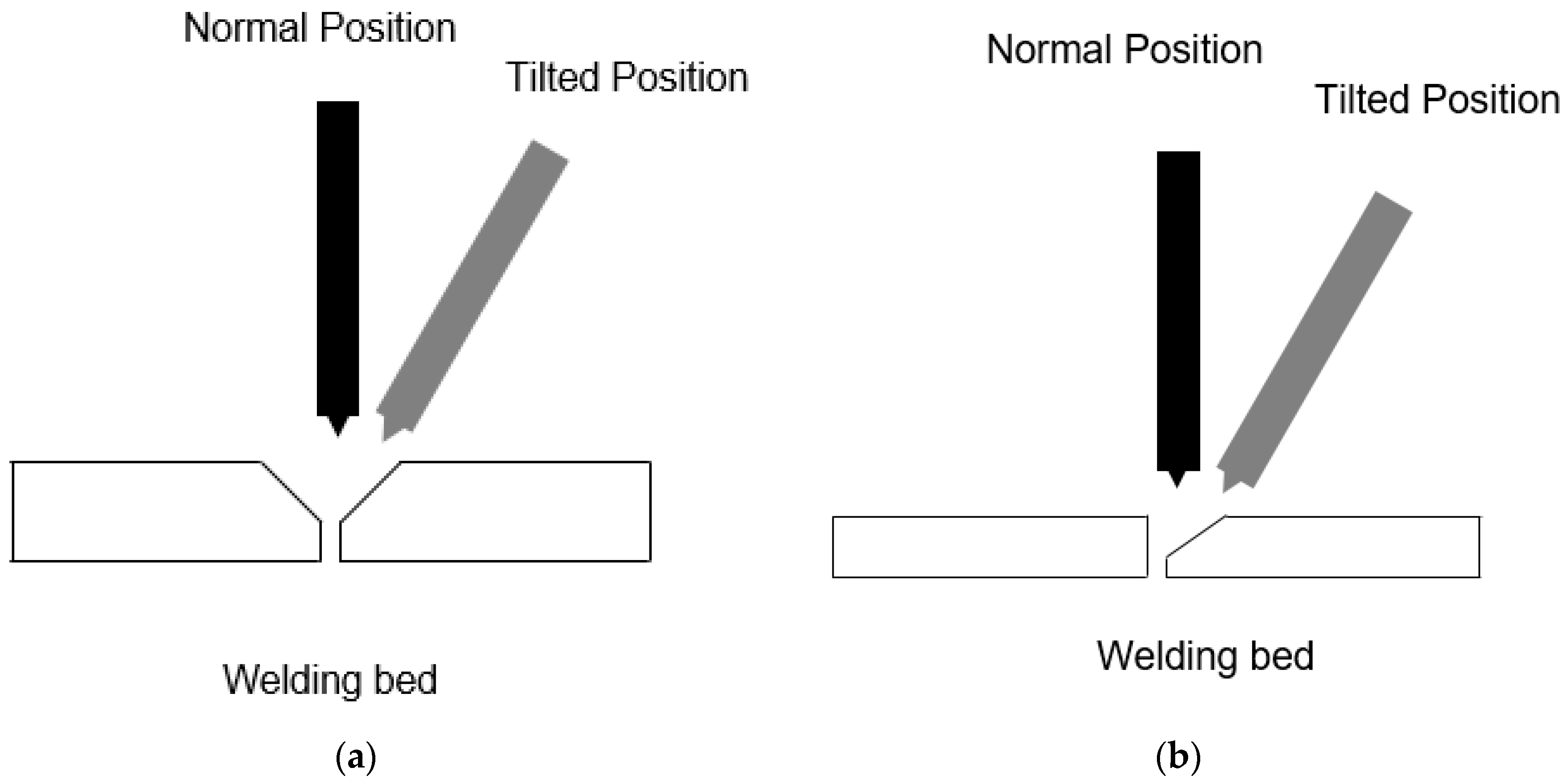
2.1. Defect Manufacturing
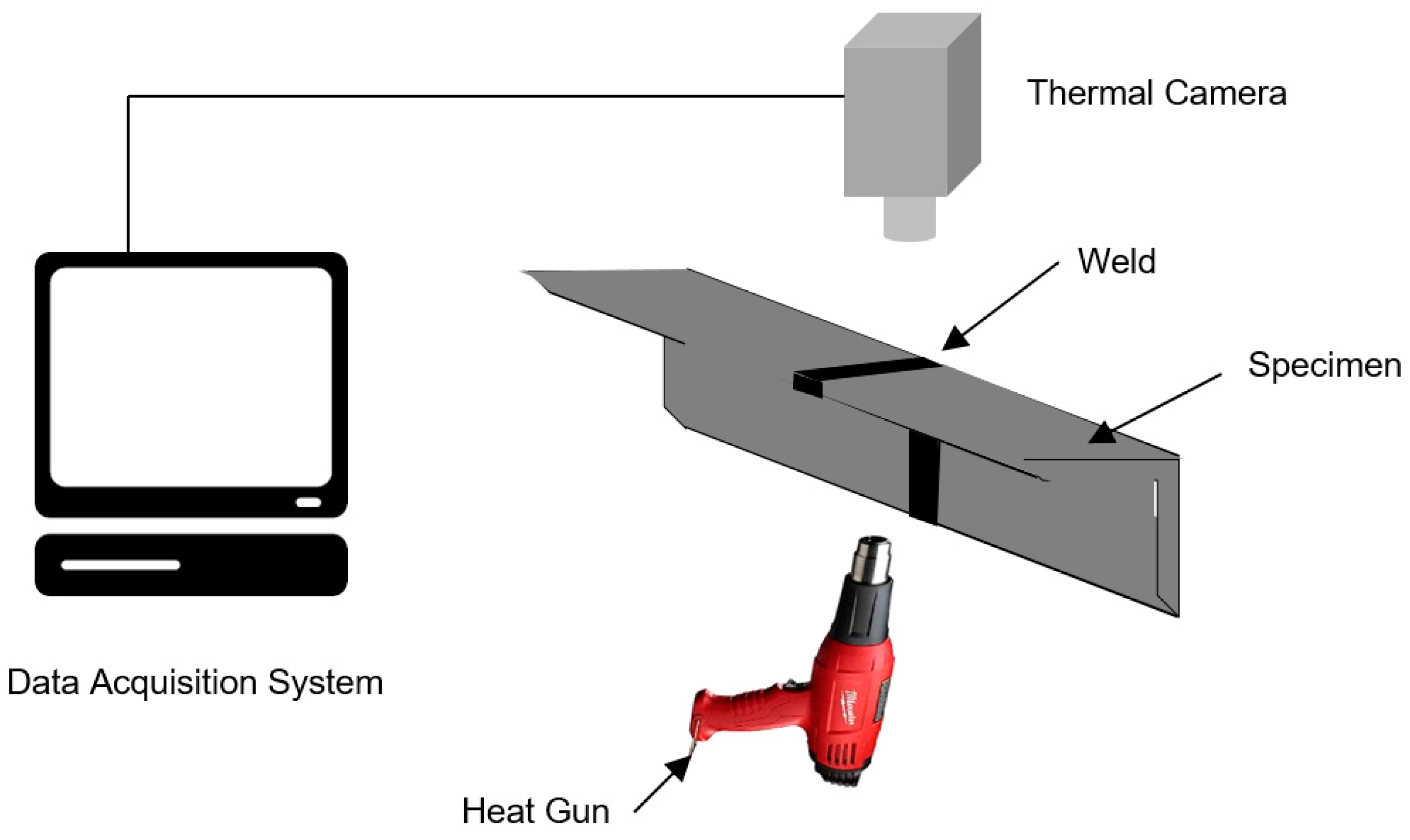
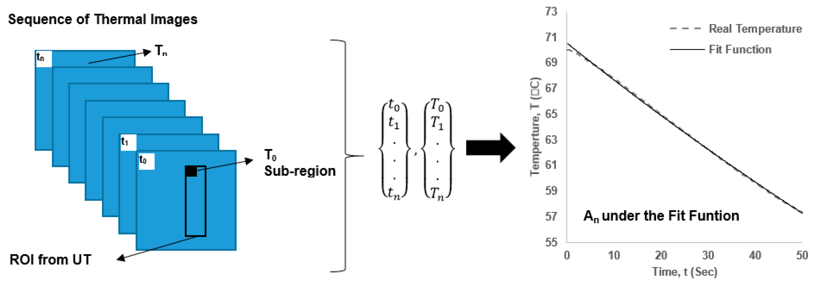
Introduction defects in weld specimens is challenging, as no precise methodology exists to control the exact location and size of a particular type of defect. In this paper, welds were manufactured to include four common defects: Inclusions, porosity, cracking, and lack of fusion. For each type of defect, a welder with experience in the open web steel joist fabrication industry used one or more technique(s) to ensure the intended defects are obtained; however, these methodologies were not always effective.
For inclusions, three methods were used. The first involved embedding a small piece of slag or ceramic into the welding bed, as seen in Figure 1. The second method utilized a 15 mm hole drilled into the wall of the base metal prior to welding (Figure 2a). The third method also utilized a drilled hole, but it was applied to the first pass of a multipass weld, as seen in Figure 2b [38].
Three techniques were used to introduce porosity into the weld specimens. Changing weld settings during the process resulted in surface porosity, as seen in Figure 3a. Adding moisture in the form of water or oil has shown to produce subsurface porosity [39]. Application of this added moisture is seen in Figure 3b,c.
To manufacture cracks, the edge of the specimen was intentionally left uneven to create an un-beveled ridge as seen in Figure 4. The un-beveled ridge imposes uneven shrinkage stresses as the weld cools, introduction the possibility of weld cracking.
Finally, to introduce the lack of fusion in the specimens, the welding contact tip was tilted from the normal position as seen Figure 5.
The surface of the final specimens in this study were not ground or prepared, consistent with US building industry standards, with the exception of two 13 mm specimens that were painted with black high emissivity paint.

2.2. IRT Method

The method used in this study is adopted from Rodríguez-Martín et al. [22] who monitored the temperature decay of the studied specimens. This method is based on Newton’s cooling law and specific heat formula which states the temperature of any given object changes in an exponential form as shown below:
T ( t ) = T a + ( T 0 T a ) e k t
where T is the temperature of a certain location at any time, T a is the ambient temperature in K, T 0 is the material temperature at the initial time in K, and k is a cooling constant in 1/s, which depends on material heat transfer constant (α) in W/m2, area of the exposed surface (A) in m2, mass of the material (m) in kg, and specific heat of the material (c) in J/kg. Equation 2 presents the relationship between the constant k and the mentioned parameters.
k = α A m c
The presence of a defect disrupts the heat transfer by changing one or multiple parameters in Equation (2). Therefore, defected regions of interest (ROIs) should theoretically have different exponential functions describing their temperature than the sound ROIs, regardless of the type of the defect. Surface defects change the exposed area whereas the sub-surface defects change the mass, c, which makes them distinctive from the sound welds.

2.3. Experimental Program

The specimens were inspected using a USN 58 L Ultrasound flaw detector (Figure 6). The inspector swept the probe along the weld to locate ROIs with defects. These ROIs manifested signal spikes in the monitor of the flaw detector. Based on the UT signal, the inspector was able to report the types and the locations of the defects. The inspector also marked the approximate locations of these defects on the specimens. The described UT inspection procedure is not the most advanced and efficient way for UT defect detection; however, it was the practiced inspection method at the manufacturer providing the weld samples.
After the UT inspection, the following IRT scheme was applied on the specimens. The specimens were heated to a temperature in the range of the operating temperature of the camera using a Milwaukee Variable Temperature Heat Gun. The heat gun increased the temperature of the specimens through transmission mode, for 8 mm specimens each leg was inspected separately. The transmission mode means the heat source and the thermal sensor are located on different sides of the specimens. Another alternative is to use the reflection mode where the heat source and the thermal sensor are located on the same side. The authors investigated both modes in a preliminary study which showed that reflection mode produced more noise due to the nature of the heat gun. Therefore, transmission mode was selected to perform the experiments. Figure 7 shows the experiment set up. The heat gun, placed within 50 mm of the bottom of the specimens, increased the temperature of the ROI, previously diagnosed with a defect by the UT inspection, in each specimen along the length of the weld.
A thermal camera was set on a tripod to monitor the surface emission of the weld. A FLIR SC640 was used as the thermal camera with an operating temperature range of −40 to 80 °C. Although this range does not correspond to temperatures occurring during the welding process, it is adequate for the purposes of examining the feasibility of IRT for in-line weld inspection. During welding, temperatures greatly exceed the operating range of the camera used in the study. However, within a matter of seconds weld temperatures typically drop below 100 °C. An IR camera following directly in-line, a few seconds behind the path of a weld, would record temperatures similar to those used in this study. The camera has a thermal sensitivity of 30 mK at 30 °C, an accuracy of ±1 °C, a spectral range of 7.5–13 μm, resolution of 640 by 480 pixels, and up to 30 Hz data acquisition frequency. When the maximum temperature in the ROI reached 70 °C, the heat gun was turned off and the camera started recording a thermal sequence with the frequency of 10 Hz for 50 s and analyzed through Therma Vision Examine IR software. The thermal camera and the specimen clearance varied for each type of specimen to ensure the ROI was captured in the thermal images. This clearance was 100 mm for the 3 mm and 8 mm specimens; and was 150 mm for the 13 mm specimens. The emissivity of the steel specimens changes with temperature; however, variation is not tangible for temperatures less than 400 °C and then the emissivity increases as the temperature rises to greater values [40]. Increase in the surface emissivity has shown to improve the IRT results in the past [41]; implying that this technique may be suitable for higher temperatures as well.
Each sequence of thermal images showed the temperature of the specimen in different locations as pixel intensities. By monitoring each pixel through time, one can fit an exponential function and compare the pixels representing sound weld to those representing defects. However, fitting a curve to each pixel in an image throughout the whole sequence can be time-consuming and computationally expensive. Therefore, sub-regions consisting of 5 by 5 pixels were arbitrarily defined for each ROI in each specimen for averaging purposes (Figure 8). The average temperature of each sub-region was then calculated and monitored in each sequence and an exponential curve was fitted to the sub-region temperatures. Averaging the temperatures on the sub-regions also has the benefit of noise reduction from the thermal sequences. In addition, the sub-regions are less sensitive to emissivity variation than the pixels of the thermal sequences. The emissivity variation has different sources but the most important one is the dark discoloration on welds [42]. Then, the area under the fitted curve function, A n , for each ROI was calculated based on the average for all the sub-regions in that ROI. The A n of each ROI can be used to recognize whether the ROI is sound or defected. For each sub-region, a general form of the exponential fit function throughout each thermal sequence, describing the temperature decay of the weld, can be obtained as follows [43].
T ( t ) = a e b t
where a and b are calculated based on the exponential interpolation, and t is time in seconds.

3. Results and Discussion

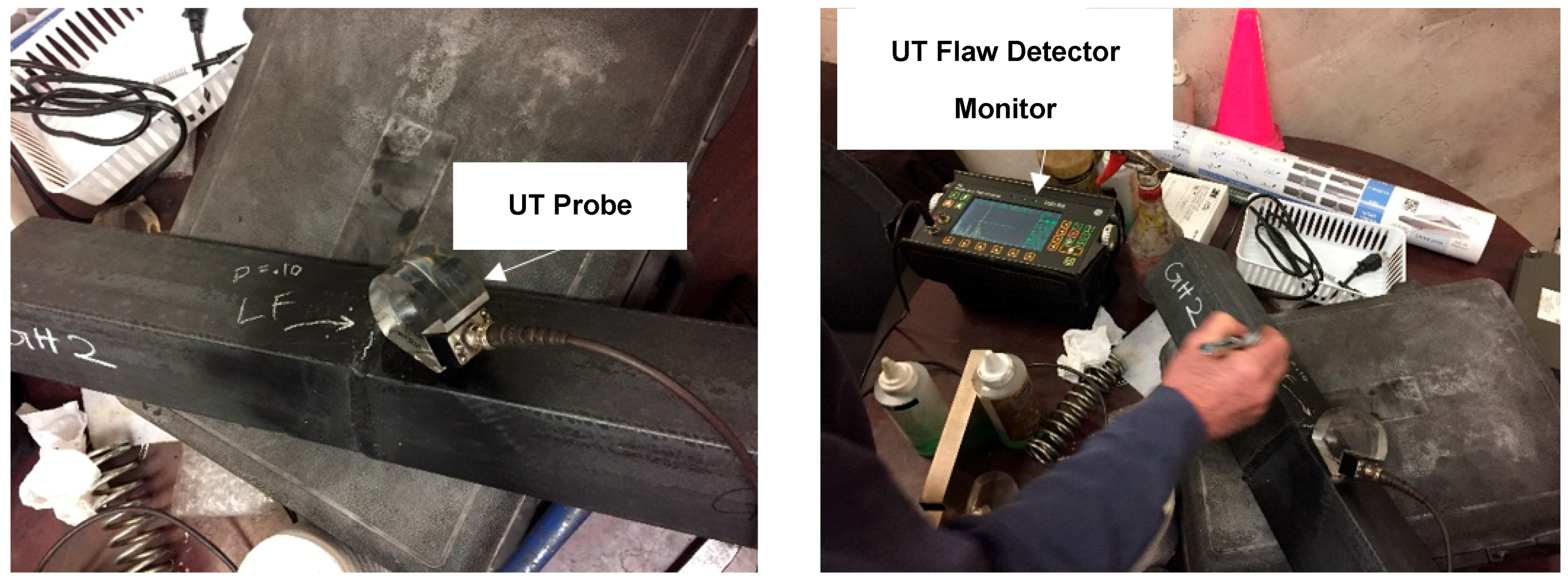
3.1. Results of the UT Inspections

The results of the UT are shown in Table 1, where quantity represents the number of specimens, an angle leg in 8 mm specimens or a plate surface the 13 mm specimens, considered to have a certain defect after the UT inspection. Each specimen was diagnosed with one defected region except for one of the 13 mm specimens which was diagnosed with three inclusions. The overpass defects reported in Table 1 were created unintentionally.

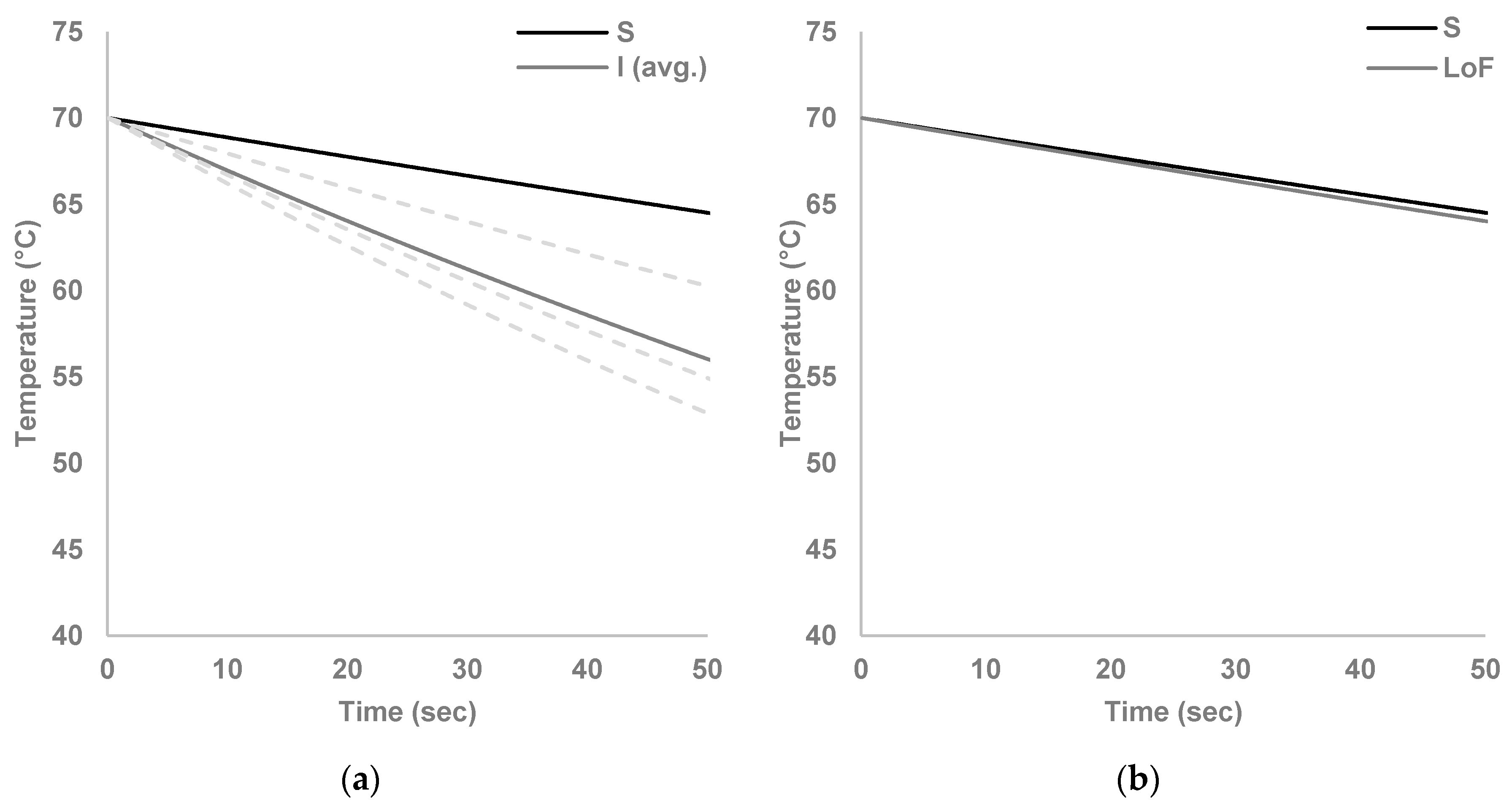
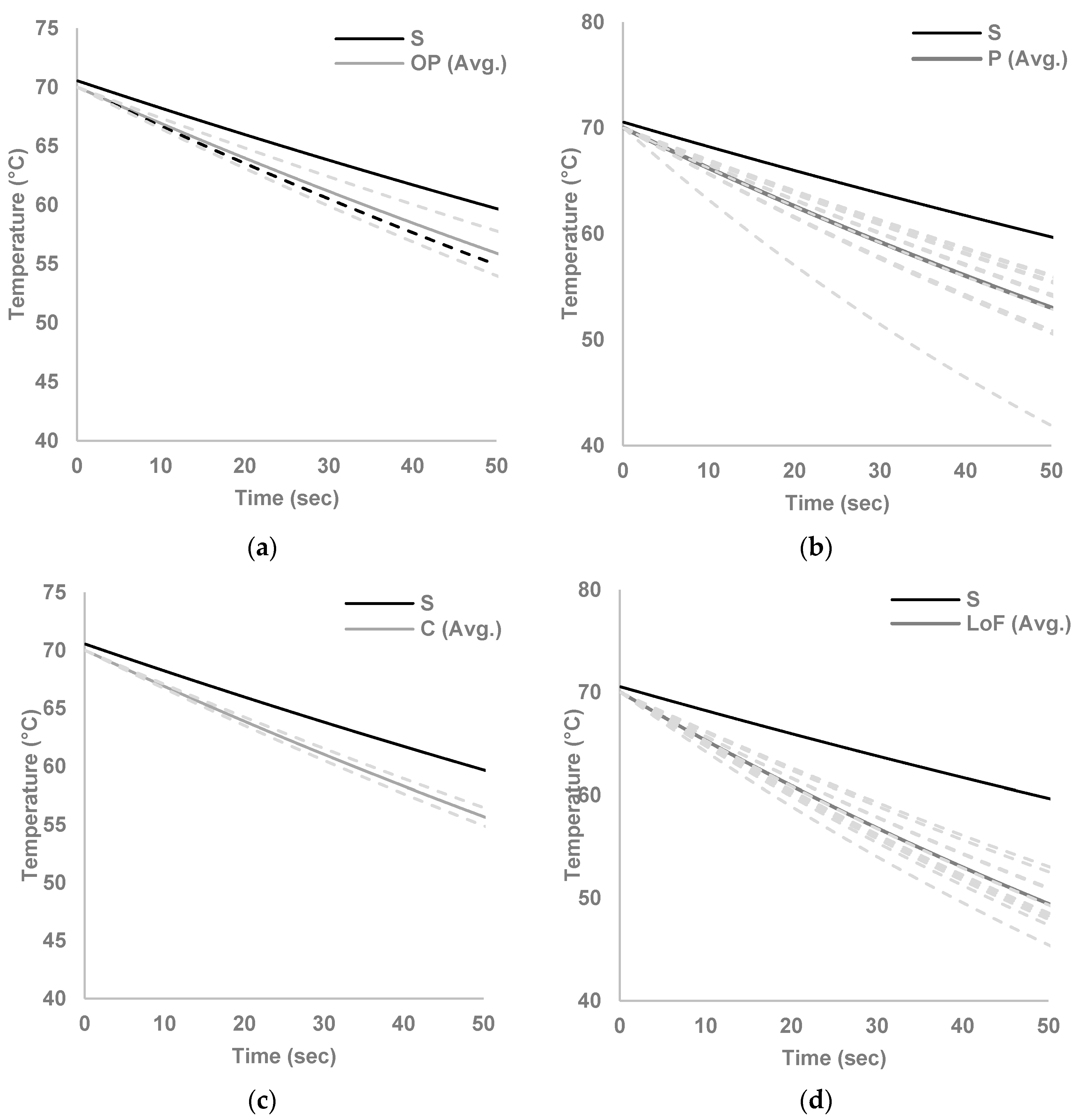
3.2. Results of the Proposed IRT Inspections

The average value of A n for the sound weld regions and the regions containing defects are shown in Table 2. The average of A n values are based on the A n values for each defected ROI for each type of defect. In addition to the average, the coefficient of variation (COV%) for the A n values associated with more than one defect is also reported in this table. The number of regions containing defects was the quantity of that defect reported in Table 1, except for the inclusion defects in the 13 mm specimen. As presented, the A n values were lower for 8 mm specimens which is reasonable since they lose the heat energy faster than the 13 mm specimens. In addition, the presence of the defects in both 13 mm and 8 mm specimens resulted in lower A n values on average, than the sound regions which means the defected ROIs lost the heat faster than the sound ones.
According to UT inspections, both 13 mm specimens contained defects. In order to find a fit function for the sound region in these specimens, two ROIs were selected in the regions that passed the UT inspection as sound. Then each ROI was segmented to several sub-regions and the fit function for each sub-region was obtained. The average A n values over all sub-regions for the 13 mm sound weld was 3354.
The UT inspection detected three inclusions in one of the 13 mm specimens and lack of fusion in the other. The temperature decay graphs of the 13 mm specimens are shown in Figure 9. The heat loss was faster in ROIs with inclusions than the sound weld as seen in Figure 9a. The gray dashed lines in Figure 9a represent the temperature decay for each ROI with inclusion and the gray solid line is the average of them. As shown, the temperature decay graph for sound weld was always above the graphs of the ROIs with inclusions. The values of A n for these inclusions were 3046, 3244 and 3102, respectively, and for lack of fusion A n was 3341. The A n for the ROI with lack of fusion was close to the A n of the sound weld, 3354, as its temperature decay graph was almost identical to the sound region temperature decay graph (Figure 9b).
Table 3 shows the average R-squared values for the fitted curves in Figure 9 along with the average a and b parameters used to generate the fit curves.
Two of the 8 mm specimens passed the UT inspections with no indications. The average A n value over all sub-regions of these specimens was 3242, and was used as the A n for sound 8 mm welds. Figure 10 shows the temperature decay graphs for each type of defect in contrast to the temperature decay graph for the sound weld. The gray dashed lines in Figure 10 represent the temperature decay graph for each ROI in Table 1, while the gray solid line shows the average. For the 8 mm specimens, the sound graph was always above the defected graphs. For porosity and lack of fusion graphs, this difference was more tangible (Figure 10b,d, respectively), than the graphs associated with inclusion and overpass (Figure 10a), and with cracking (Figure 10c).
Table 4 shows the average R-squared values for the fitted curves in Figure 10 along with the average a and b parameters used to generate the fit curves.

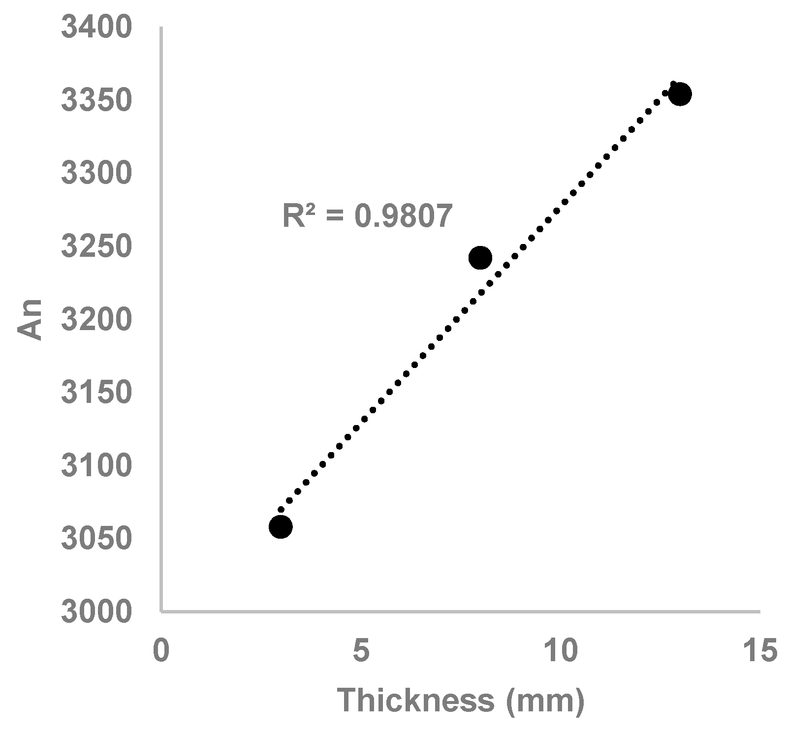
3.3. Using the Proposed IRT Method for the 3 mm Specimens

As previously discussed, UT inspection is not valid for the 3 mm specimens. However, two welds made using typical processes were selected as control specimens, assumed to be sound welds with no defects. The average A n value over the selected sub-regions of these specimens was 3056. The mean value of the coefficients in Equation (3) for the 3 mm sound specimens were a = 69.8, b = 0.0045. Figure 11 shows the A n value for sound welds obtained in this study for 3 mm, 8 mm, and 13 mm specimens. A line was fit to the points in this figure and shows a linear correlation between the specimen thickness and average A n values for the sound welds. This extrapolation ensures the selected A n value for the 3 mm control specimens was within a reasonable range since UT inspection was unable to confirm the quality of these specimens.
The remaining six 3 mm specimens were fabricated with flaws: One with cracking, three with porosity, one with lack of fusion, and one with inclusion. The 3 mm specimens went through the same IRT procedure described previously. However, a notable difference between the procedures is that the inspection covered the whole weld surface instead of ROIs indicated by UT to contain defects. Then, the A n values for all the sub-regions in each ROI was calculated and compared to 3056. Sub-regions with A n less than 3056 were considered to have defects and were highlighted in Figure 12. Only three of the six specimens had A n values less than 3056. The specimen in Figure 12a was manufactured to have lack of fusion however the detect pattern by the IRT suggested either porosity or inclusions. Figure 12b shows the specimen manufactured with porosity, and the IRT method predicted a similar pattern. The specimen shown in Figure 12c was also manufactured to have porosity; however, the IRT method predicted a pattern similar to lack of fusion.

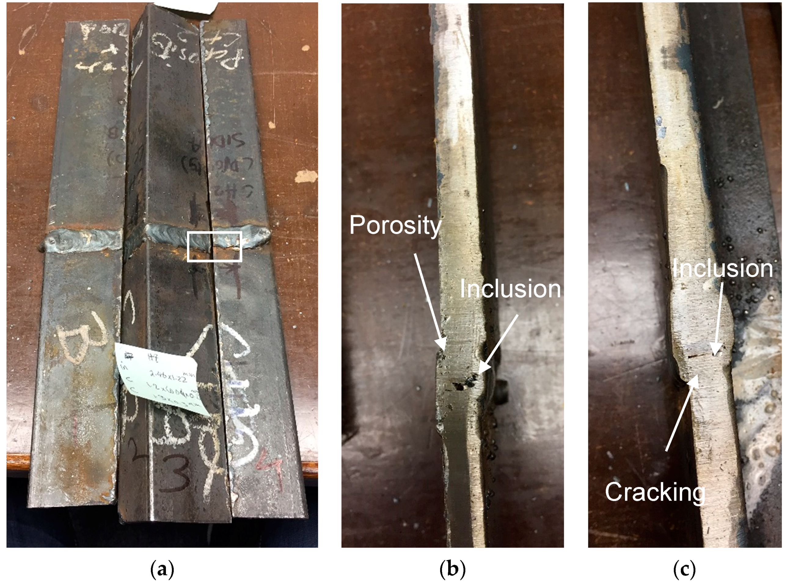
3.4. Destructive Testing

Destructive testing was performed on all weld specimens to confirm the location of defects, and included cutting the weld specimens longitudinally at susceptible locations. The susceptible locations are determined in the UT inspections and confirmed by the IRT technique for 8 mm and 13 mm specimens. Figure 13 shows the cut of one of the 8 mm specimens. As shown in the Figure 13b,c, the methods used for defect manufacturing did not always result in the intended defects. However, the cuts confirmed the presence of one or more weld defects at the all the ROIs examined by UT inspection, except for three ROIs, two in 13 mm specimens and one in 8 mm specimens. However, this does not mean that the fabrication methodologies failed to manufacture the defect. Due to the small size of the defects and the difficulty in precisely defining their location, cuts may have missed defects. Examples of defects identified by destructive testing are seen in Figure 13a, where the ROI is shown with a box on the one of the cuts.

3.5. Challenges to Implementation

Results of the current study show the feasibility of IRT for weld inspection and defect detection. Although the temperatures used in this study do not reach maximum temperatures recorded during the welding process, they do mimic realistic weld temperatures for cooling ranges typical to structural welds. The IRT method for weld defect detection can identify the locations of defects, the regions with smallest values of A n . However, many challenges still exist and must be overcome as researchers work towards implementation IRT inspection for in-line, real-time weld inspection. Based on the results of the current study, authors have identified the following challenges associated with the proposed methodology. More investigations are required in the future to address these challenges before this method can be used effectively.

3.5.1. Weld Surface

During the welding process, irregularities were produced on specimen surfaces. These irregularities, including both geometric bumps and color contrast, affected the thermal images. These irregularities were not associated with the presence of defects in the welds and could mislead the inspector viewing the captured thermal images. The presence of these irregularities can increase the false positive detections in a thermal image. Having these irregularities changes the surface emissivity of the material and can cause inaccuracy in the camera readings. This issue is even more important when dealing with low-emissivity materials such as steel. It is possible to grind the weld surface to get rid of the surface clutters and bumps but it would not be practical in some manufacturing processes. Scarfing, an often automated process in which excess material can be torched or chipped from the surface, may be used in the future for certain member geometries which is significantly less time-consuming than manual grinding, which is common in the bridge fabrication industry. Another option is covering the weld surface with high emissivity paint to provide a mono-contrast surface for thermography. This would also likely fit easily into the manufacturing process and could even be semi-automated. All welds eventually get painted in the manufacturing process. However, this would limit the realtime inspection provided by the IRT as painting cannot be performed on hot specimens.

3.5.2. Emissivity Control

The surface emissivity varies as the temperature of the specimen changes. Even though this change was not significant in the temperature range studied in this paper, it could alter the results for realtime applications when the temperature ranges are higher. Performing an investigation to determine the surface emissivity of the welded specimens in a temperature range of 1000 to 4000 °C could be very helpful to calibrate the proposed IRT method. In order to determine the emissivity, the methodology used in reference [40] can be replicated. However, even with this information, surface emissivity will be significantly affected by the non-uniform weld surface.

3.5.3. Camera

The specifications of the infrared camera play an important role in IRT weld inspection. The camera used for this study, FLIR SC 640, is not ideal in terms of resolution, sampling rate, and sensitivity. However, the most important issue with the FLIR SC 640 was its temperature range (−40 to 80 °C). Although this range allows for the recording of weld temperatures a few seconds after cooling, a camera with a higher temperature range would allow for more flexibility with the inspection procedure. Other camera models, including the FLIR SC 6100, measure up to 2000 °C and can record sequences up to 126 Hz, making them more appropriate for weld inspection using only the heat generated by the welding process. Various commercially-available cameras are manufactured with even larger temperature ranges.

3.5.4. Uncontrolled and Uneven Heating

Excitation source is another factor affecting the success of IRT weld inspection. In this study, a heat gun was used to simulate the temperature condition of a steel angle after welding in a lower scale. The heat gun provides a cheap, easy-to-use, and repeatable source for increasing the temperature of the welds; however, the transmitted energy from the heat gun is not homogenous. Functionally, some regions get hotter than the others. This mimics in-line weld inspections since the weld surface has different temperatures right after welding is performed. However, the heat unevenness will reduce as the specimen cools down after 2–5 min of manufacturing according to the authors’ observations. Using even heat sources in the future could mimic the weld-surface a few minutes after manufacturing which still would be an improvement over the four-hours wait time.

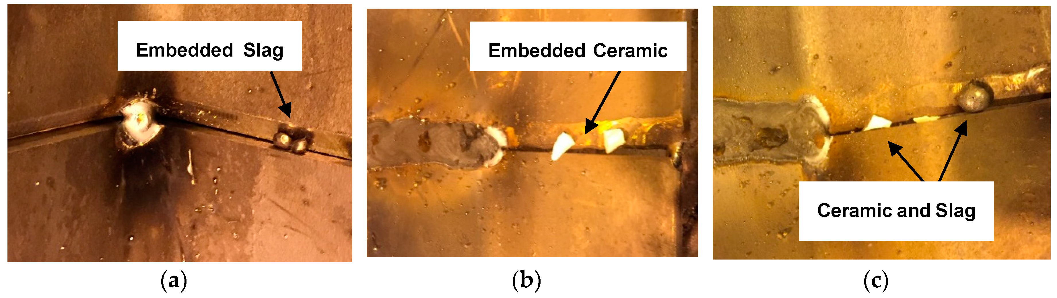
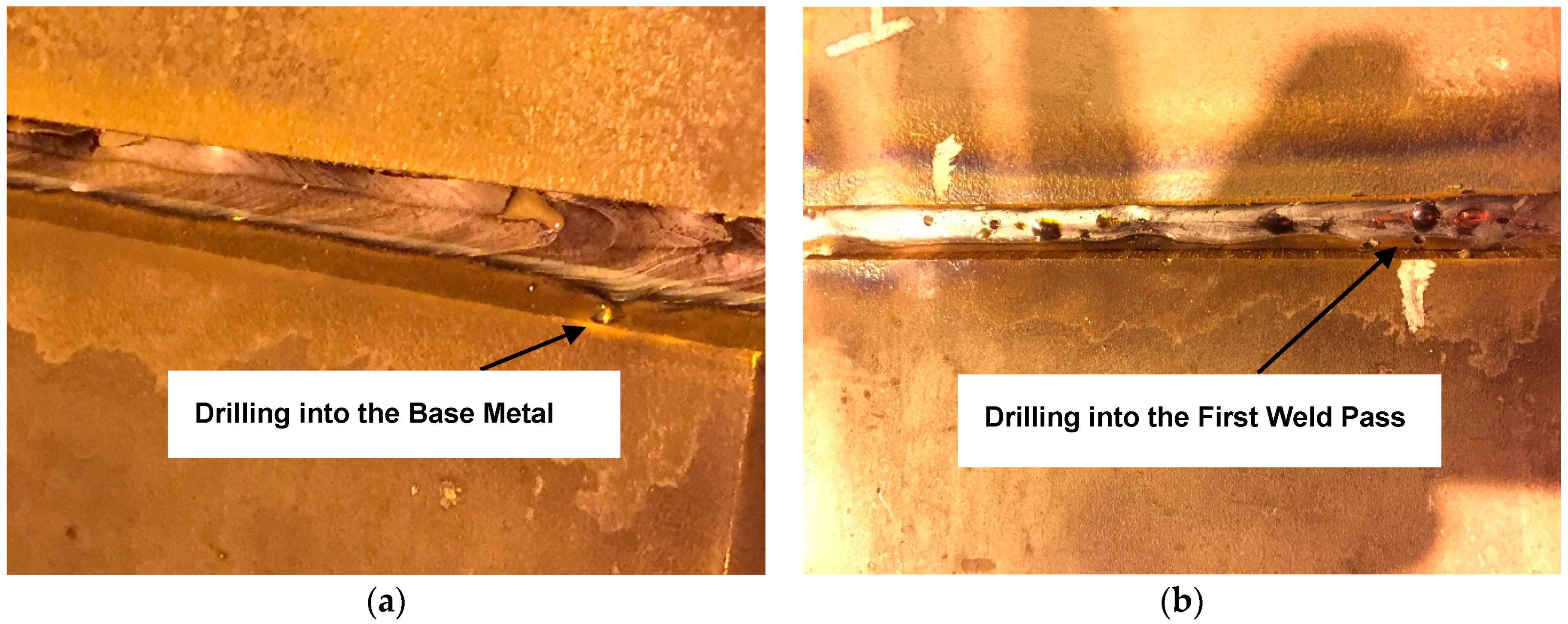
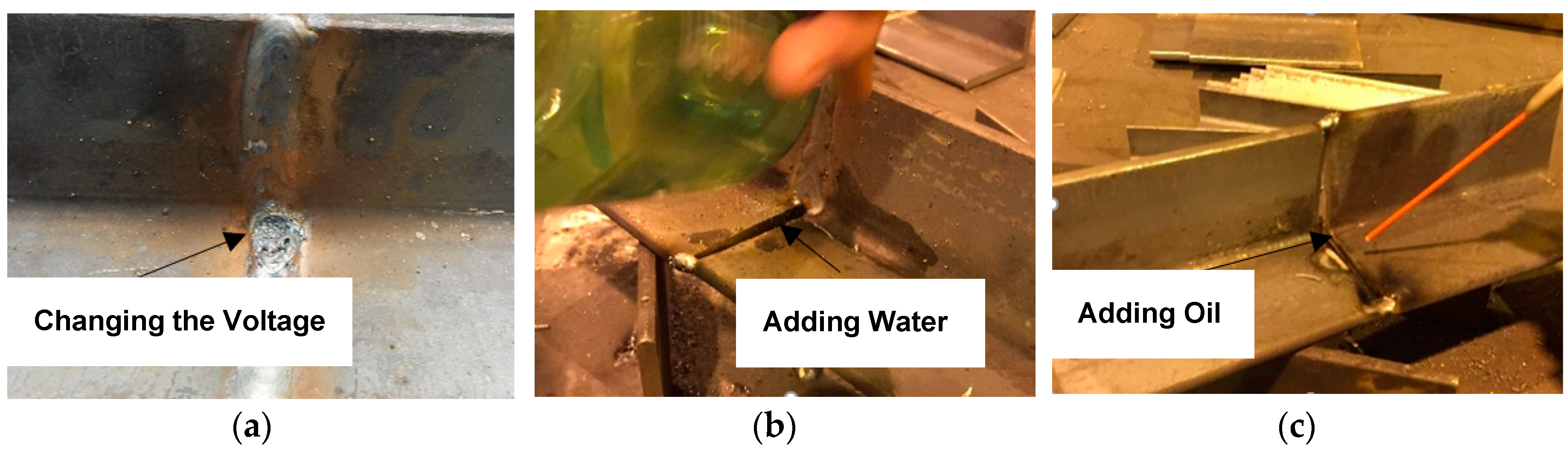
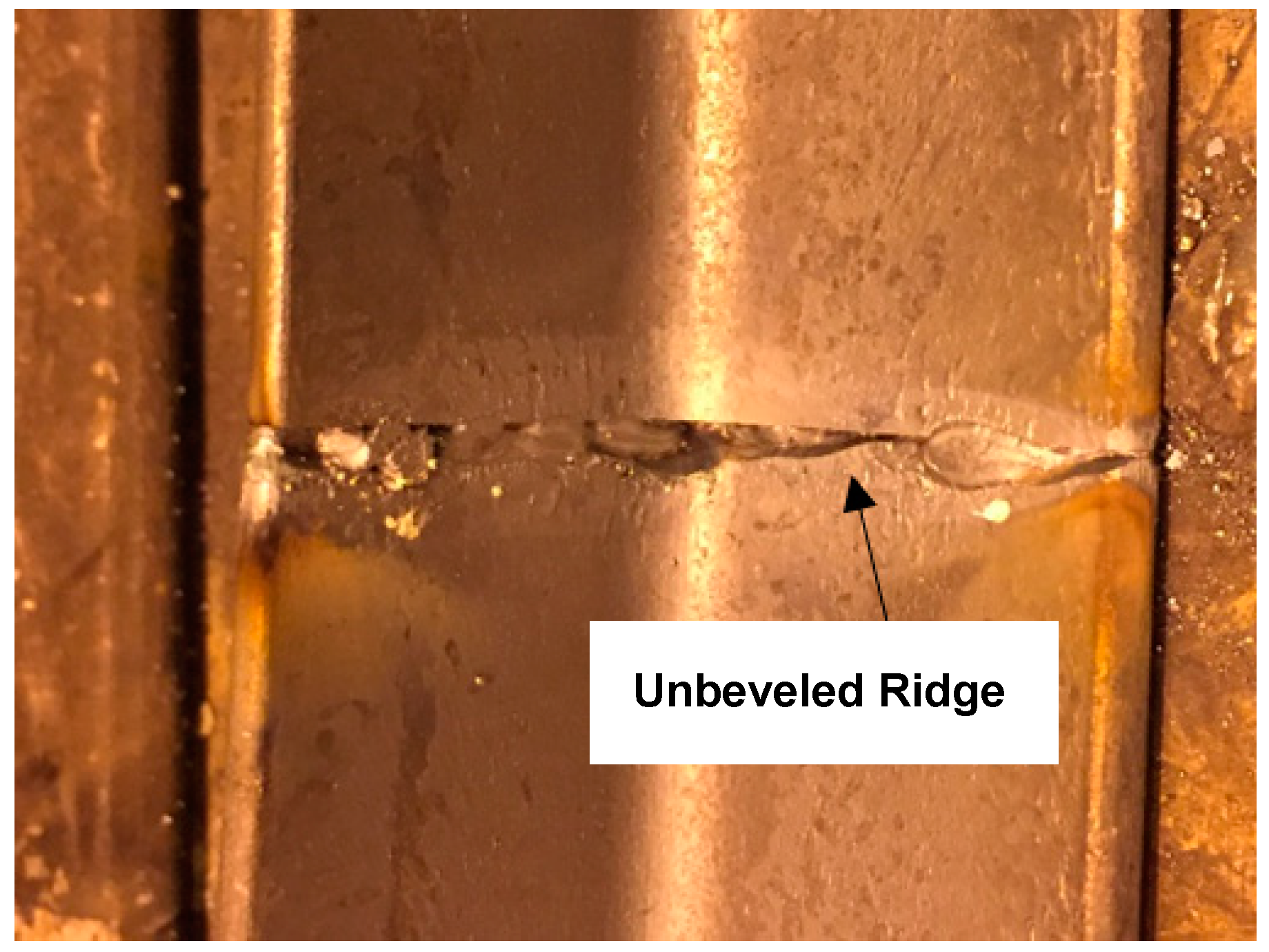
3.5.5. Defect Manufacturing

The methodologies used to generate defects could be improved to be more precise and controlled. Lack of fusion aside, porosity seemed to be the most convenient defect to manufacture by introducing water and oil to the weld path; however, most of the obtained porosities were on the surface and visually detectable which does not represent the porosities in the real welds that need NDE. Although consistent and predictable defect manufacturing is necessary in all weld inspection research, the literature shows that this is a major challenge for almost all weld inspection validation studies [38].

3.5.6. Welding Process

The process used to create the welds in this study was globular transfer which is the standard method in the joist manufacturing industry. However, it is a manual process, resulting in uneven surface quality of the welds and splatter negatively affecting variability of surface emissivity. Tungsten inert gas (TIG) welding can be used to create the defects in a more controlled manner to calibrate the proposed IRT method for defect detection in different weld transfer modes.

4. Conclusions

Verification of weld workmanship and structural performance is paramount to weld inspection both during fabrication and in-service. Weld inspections are costly in terms of time and money for both situations. Ultrasonic testing (UT) has been widely used to detect surface and sub-surface defects of welds. Like other non-destructive methods, UT is an inspection with contact which leads to wait-times up to 4 h for the specimens to cool down before any inspections can take place. This adds time, storage requirements, and, consequently cost to the inspection process. This paper proposes using infrared thermography (IRT) in weld inspection, particularly for sub-surface defect detection. IRT is a non-contact method and has the potential to be applied for weld inspection using a high-temperature range thermal camera.
Four common weld defects were made to be detected including inclusion, porosity, cracking, and lack of fusion. The studied specimens included two plates with a thickness of 13 mm, 14 angles with a thickness of 8 mm, and eight angles with a thickness of 3 mm. An inspector determined the regions with defects through UT inspections in 13 mm and 8 mm specimens. The specimens then were heated using a heat gun in heat transmission mode. A thermal camera was set on a tripod and monitored the surface emission of the weld. When the maximum temperature in regions of interest, i.e., the susceptible regions, on the weld neared 70 °C, the heat gun was turned off and the camera started recording thermal sequences with a 10 Hz frequency for 50 s. The recorded sequences were then analyzed to find the rate at which sub-regions in each ROI lost heat by fitting an exponential fit function and calculating the area under this function ( A n ).
Results indicate the sound welds had larger values of A n than the welds with defects. Results of the UT and IRT inspections closely matched, proving the feasibility of using IRT for weld inspections. As per ASTM standards, UT inspection was not an option for the 3 mm specimens. Therefore, two specimens were fabricated under ideal conditions to be control specimens. These were analyzed to obtain A n for sound welds. The sub-regions with areas less than sound weld A n were identified as defected regions. Possible porosity and lack of fusion were detected by this method in three specimens, while no defects were detected in the other three. In addition, the destructive testing confirmed the presence of lack of fusion detected by the IRT method.
Challenges associated with using IRT for weld inspection were as follows:
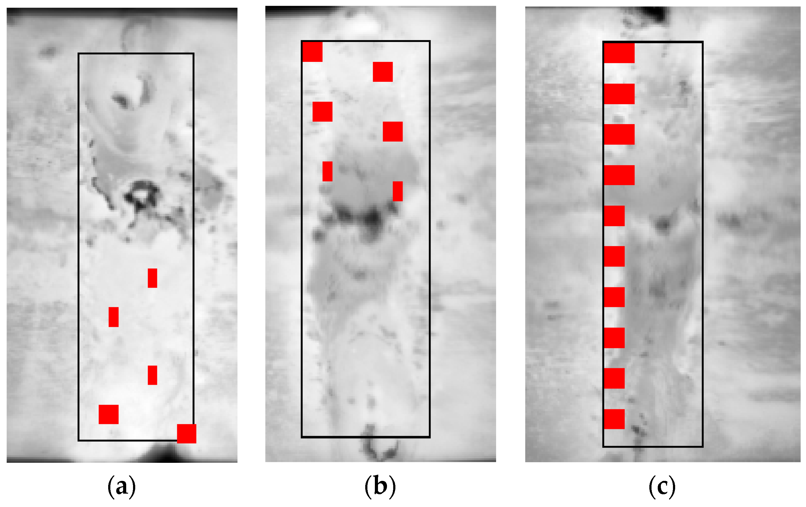
  • Surface clutter and the uneven surface created during welding were not related to the presence of defects in the welds, but they can be misleading in the captured thermal images. Having this clutter changes the surface emissivity of the material and can cause inaccuracy in the camera readings, especially in low-emissivity materials.
  • The camera used for this study, FLIR SC 640, only measures temperature in the range of −40 to 80 °C, which limits the application for in-line weld inspections.
  • Using the fit function of the temperature decay for a five by five sub-region instead of using actual temperatures presented in each pixel alleviated the effects of un-even heating and surface clutters to some extent, but did not completely resolve them. This condition is also similar to the conditions that would exist during in-line inspections using only the heat generated by the welding process.
  • Despite using standard methods to fabricate defects, some were hard to create, including cracks and inclusions. The manufactured porosities were mostly on the material surface instead of sub-surface. Lack of fusion was manifested in welds when it was not supposed to; either they were built to have a different defect or no defects at all.
For further study and inspection, the following recommendations are proposed:
  • Using high temperature range cameras coupled with a data acquisition system and software.
  • Continue to develop methods for reliable and quantifiable defect fabrication.
  • Examine the applicability of IRT weld inspection to other weld processes, including both automatic and semi-automatic processes.
  • Using controlled heat sources to excite the specimens, such as high power halogen or UV lamps.
  • Using the inherent heat from the welding process for a real-world study of in-line weld inspection.

Author Contributions

Conceptualization, S.D., M.M., W.C.; Methodology, S.D.; Software, S.D.; Validation, S.D., M.M., W.C.; Formal Analysis, S.D.; Investigation, S.D.; Resources, M.M.; Data Curation, S.D.; Writing-Original Draft Preparation, S.D.; Writing-Review & Editing, S.D., M.M., W.C.; Visualization, S.D.; Supervision, M.M.; Project Administration, M.M.; Funding Acquisition, M.M.

Funding

This research was funded by Vulcraft Corporation.

Conflicts of Interest

The authors declare no conflict of interest.

References

  1. Liao, T.W.; Li, Y. An automated radiographic NDT system for weld inspection: Part II-Flaw Detection. NDT E Int. 1998, 31, 183–192. [Google Scholar] [CrossRef]
  2. Wang, G.; Liao, T.W. Automatic identification of different types of welding defects in radiographic images. NDT E Int. 2002, 35, 519–528. [Google Scholar] [CrossRef]
  3. Yusa, N.; Janousek, L.; Rebican, M.; Chen, Z.; Miya, K.; Chigusa, N.; Ito, H. Detection of embedded fatigue cracks in Inconel weld overlay and the evaluation of the minimum thickness of the weld overlay using eddy current testing. Nuclear Eng. Des. 2006, 236, 1852–1859. [Google Scholar] [CrossRef]
  4. Smid, R.; Docekal, A.; Kreidl, M. Automated classification of eddy current signatures during manual inspection. NDT E Int. 2005, 38, 462–470. [Google Scholar] [CrossRef]
  5. Jiles, D.C. Review of magnetic methods for nondestructive evaluation (Part 2). NDT Int. 1990, 23, 83–92. [Google Scholar] [CrossRef]
  6. Ditchburn, R.J.; Burke, S.K.; Scala, C.M. NDT of welds: State of the art. NDT E Int. 1996, 29, 111–117. [Google Scholar] [CrossRef]
  7. Buttram, J. Ultrasonic Method for the Accurate Measurement of Crack Height in Dissimilar Metal Welds Using Phased Array. U.S. Patent Application 11/030,365, 4 January 2007. [Google Scholar]
  8. Latimer, P.J.; MacLauchlan, D.T. EMAT Probe and Technique for Weld Inspection. U.S. Patent 5,760,307, 2 June 1998. [Google Scholar]
  9. Petcher, P.A.; Dixon, S. Weld defect detection using PPM EMAT generated shear horizontal ultrasound. NDT E Int. 2015, 74, 58–65. [Google Scholar] [CrossRef]
  10. Rasooli, B. Inspection-for-Industry.com. Available online: https://www.inspection-for-industry.com/radiographic-testing.html (accessed on 17 August 2018).
  11. Hayes, C. The ABC’s of nondestructive weld examination. Weld. J. 1997, 76, 45–51. [Google Scholar]
  12. Lhémery, A.; Calmon, P.; Lecœur-Taıbi, I.; Raillon, R.; Paradis, L. Modeling tools for ultrasonic inspection of welds. NDT E Int. 2000, 33, 499–513. [Google Scholar] [CrossRef]
  13. Kim, K.; Kang, S.; Kim, W.; Cho, H.; Park, J. Improvement of radiographic visibility using an image restoration method based on a simple radiographic scattering model for x-ray nondestructive testing. NDT E Int. 2018, 98, 117–122. [Google Scholar] [CrossRef]
  14. Rao, B.P.; Raj, B.; Jayakumar, T.; Kalyanasundaram, P. An artificial neural network for eddy current testing of austenitic stainless steel welds. NDT E Int. 2002, 35, 393–398. [Google Scholar] [CrossRef]
  15. Bagavathiappan, S.; Lahiri, B.B.; Saravanan, T.; Philip, J.; Jayakumar, T. Infrared thermography for condition monitoring—A review. Infrared Phys. Technol. 2013, 60, 35–55. [Google Scholar] [CrossRef]
  16. Elert, G. The Physics Factbooks. 2003. Available online: https://hypertextbook.com/facts/2003/EstherDorzin.shtml (accessed on 26 August 2018).
  17. ASTM International. Standard Practice for Contact Ultrasonic Testing of Weldments; ASTM E164-13; ASTM International: West Conshohocken, PA, USA, 2013. [Google Scholar]
  18. Broberg, P. Surface crack detection in welds using thermography. NDT E Int. 2013, 57, 69–73. [Google Scholar] [CrossRef]
  19. Li, T.; Almond, D.P.; Rees, D.A.S. Crack imaging by scanning pulsed laser spot thermography. NDT E Int. 2011, 44, 216–225. [Google Scholar] [CrossRef]
  20. Meola, C.; Carlomagno, G.M.; Squillace, A.; Giorleo, G. The use of infrared thermography for nondestructive evaluation of joints. Infrared Phys. Technol. 2004, 46, 93–99. [Google Scholar] [CrossRef]
  21. Schlichting, J.; Brauser, S.; Pepke, L.A.; Maierhofer, C.; Rethmeier, M.; Kreutzbruck, M. Thermographic testing of spot welds. NDT E Int. 2012, 48, 23–29. [Google Scholar] [CrossRef]
  22. Rodríguez-Martín, M.; Lagüela, S.; González-Aguilera, D.; Arias, P. Cooling analysis of welded materials for crack detection using infrared thermography. Infrared Phys. Technol. 2014, 67, 547–554. [Google Scholar] [CrossRef]
  23. Tang, Q.; Liu, J.; Wang, Y.; Liu, H. Subsurface interfacial defects of metal materials testing using ultrasound infrared lock-in thermography. Procedia Eng. 2011, 16, 499–505. [Google Scholar] [CrossRef]
  24. Lee, S.; Nam, J.; Hwang, W.; Kim, J.; Lee, B. A study on integrity assessment of the resistance spot weld by Infrared Thermography. Procedia Eng. 2011, 10, 1748–1753. [Google Scholar] [CrossRef]
  25. Plum, R.; Ummenhofer, T. Ultrasound excited thermography of thickwalled steel load bearing members. Quant. Infrared Thermogr. J. 2009, 6, 79–100. [Google Scholar] [CrossRef]
  26. Renshaw, J.B.; Glass, S.W., III; Thigpen, B.A.; Taglione, M. Vibrothermographic Weld Inspections. U.S. Patent 9,146,205, 29 September 2015. [Google Scholar]
  27. Plum, R.; Ummenhofer, T. Use of ultrasound excited thermography applied to massive steel components: Emerging crack detection methodology. J. Bridge Eng. 2011, 18, 455–463. [Google Scholar] [CrossRef]
  28. Garrido, I.; Laguela, S.; Arias, P. Infrared Thermography’s Application to Infrastructure Inspections. Infrastructures 2018, 3, 35. [Google Scholar] [CrossRef]
  29. Maldague, X.; Galmiche, F.; Ziadi, A. Advances in pulsed phase thermography. Infrared Phys. Technol. 2002, 43, 175–181. [Google Scholar] [CrossRef]
  30. Schönberger, A.; Virtanen, S.; Giese, V.; Schröttner, H.; Spießberger, C. Non-destructive detection of corrosion applied to steel and galvanized steel coated with organic paints by the pulsed phase thermography. Mater. Corros. 2012, 63, 195–199. [Google Scholar] [CrossRef]
  31. Roche, J.M.; Leroy, F.H.; Balageas, D.L. Images of thermographic signal reconstruction coefficients: A simple way for rapid and efficient detection of discontinuities. Mater. Eval. 2014, 72, 73–82. [Google Scholar]
  32. Maldague, X.P. Introduction to NDT by active infrared thermography. Mater. Eval. 2002, 60, 1060–1073. [Google Scholar]
  33. Usamentiaga, R.; Venegas, P.; Guerediaga, J.; Vega, L.; Molleda, J.; Bulnes, F.G. Infrared thermography for temperature measurement and non-destructive testing. Sensors 2014, 14, 12305–12348. [Google Scholar] [CrossRef] [PubMed]
  34. Runnemalm, A.; Ahlberg, J.; Appelgren, A.; Sjökvist, S. Automatic inspection of spot welds by thermography. J. Nondestruct. Eval. 2014, 33, 398–406. [Google Scholar] [CrossRef]
  35. Rajic, N. Principal component thermography for flaw contrast enhancement and flaw depth characterisation in composite structures. Compos. Struct. 2002, 58, 521–528. [Google Scholar] [CrossRef]
  36. Manuel, M.V.; Washer, G. Use of Infrared Thermography for the Inspection of Welds in the Shop and Field; No. FDOT BDV31-977-64; Transportation Research Board: Washington, DC, USA, 2017. [Google Scholar]
  37. Sakagami, T.; Izumi, Y.; Kobayashi, Y.; Mizokami, Y.; Kawabata, S. Applications of Infrared Thermography for Nondestructive Testing of Fatigue Cracks in Steel Bridges. In Proceedings of the Thermosense: Thermal Infrared Applications XXXVI, Bellingham, WA, USA, 21 May 2014. [Google Scholar]
  38. Consonni, M.; Wee, C.F.; Schneider, C. Manufacturing of welded joints with realistic defects. Insight Non Destr. Test. Cond. Monit. 2012, 54, 76–81. [Google Scholar] [CrossRef]
  39. Kemppainen, M.; Virkkunen, I.; Pitkanen, J.; Paussu, R.; Hanninen, H. Realistic Cracks for In-Service Inspection Qualification Mock-Ups. J. Nondestruct. Test. 2003, 8, 1–8. [Google Scholar]
  40. Sadiq, H.; Wong, M.B.; Tashan, J.; Al-Mahaidi, R.; Zhao, X.L. Determination of steel emissivity for the temperature prediction of structural steel members in fire. J. Mater. Civ. Eng. 2012, 25, 167–173. [Google Scholar] [CrossRef]
  41. Vollmer, M.; Möllmann, K.P. Infrared Thermal Imaging: Fundamentals, Research and Applications; John Wiley & Sons: Hoboken, NJ, USA, 2017. [Google Scholar]
  42. Jonietz, F.; Myrach, P.; Suwala, H.; Ziegler, M. Examination of spot welded joints with active thermography. J. Nondestruct. Eval. 2016, 35. [Google Scholar] [CrossRef]
  43. Leike, A. Demonstration of the exponential decay law using beer froth. Eur. J. Phys. 2001, 23, 21–26. [Google Scholar] [CrossRef] [Green Version]
Figure 1. Manufacturing inclusion in the welds using (a) embedded slag, (b) embedded ceramic, and (c) embedded ceramic and slag.
Infrastructures 03 00045 g001
Figure 2. Manufacturing inclusion in the welds using drilling in (a) base metal and (b) first pass of weld.
Infrastructures 03 00045 g002
Figure 3. Manufacturing porosity in the welds by (a) changing voltage settings, (b) adding water, (c) adding oil (WD-40).
Infrastructures 03 00045 g003
Figure 4. Manufacturing cracks in the welds by leaving out a part of the bevels.
Infrastructures 03 00045 g004
Figure 5. Weld manufacturing with lack of fusion (a) double beveled, (b) single beveled.
Infrastructures 03 00045 g005
Figure 6. Ultrasonic testing (UT) inspection using USN 58 L Ultrasonic flaw detector.
Infrastructures 03 00045 g006
Figure 7. Schematic representation of infrared thermography (IRT) inspection attempting simulation of weld inspection.
Infrastructures 03 00045 g007
Figure 8. Schematic representation of the proposed method.
Infrastructures 03 00045 g008
Figure 9. Temperature decay for 13 mm specimens (a) inclusion, (b) lack of fusion.
Infrastructures 03 00045 g009
Figure 10. Temperature decay for 8 mm specimens (a) overpass and inclusion, (b) porosity, (c) cracking, (d) lack of fusion.
Infrastructures 03 00045 g010
Figure 11. The relationship between A n values for the sound weld and the thickness of the specimen.
Infrastructures 03 00045 g011
Figure 12. The predicted defects in the 8 mm specimens (a) lack of fusion intended specimen with suggested porosity or inclusion, (b) porosity intended specimen suggesting porosity or inclusion, (c) porosity specimen suggesting lack of fusion. Red highlight indicates IRT method identified defects, black boxes indicate the region of interest.
Infrastructures 03 00045 g012
Figure 13. Destructive testing result example, (a) longitudinal cut, (b) inclusion and porosity, (c) inclusion and cracks.
Infrastructures 03 00045 g013
Table 1. Results of the UT inspections.
Specimen NumberSpecimen Thickness (mm)Detected Defect
113Inclusion (I)
2Lack of Fusion (LoF)
38Inclusion (I)
4–15Porosity (P)
16–17Cracking (C)
18–28Lack of Fusion (LoF)
29–30Overpass (OP)
Table 2. Area under the fit function ( A n ) values for the specimens.
Specimen Thickness (mm)Defect (ID) A n (Avg.) A n (COV%)
13Sound (S)3354NA
Inclusion (I)31303.2
8Lack of fusion (LoF)3341NA
Sound (S)3242NA
Inclusion (I)3102NA
Porosity (P)30473.9
Cracking (C)31221.0
Lack of fusion (LoF)29392.7
Overpass (OP)31382.3
Table 3. Stats for the 13 mm specimens.
ValueSoundInclusionLack of Fusion
R2 (avg.)0.96 *0.970.98 *
a (avg.)70 *70.170 *
a (COV%)NA *0.013NA *
b (avg.)0.00196 *0.004100.00202 *
b (COV%)NA *32.72NA *
* One sample.
Table 4. Stats for the 8 mm specimens.
ValueSoundInclusionOverpassPorosityCrackingLack of Fusion
R2 (avg.)0.94 *0.96 *0.930.930.970.96
a (avg.)70 *70 *70707070
a (COV%)NA *NA *0.010.0050.020.01
b (avg.)0.00377 *0.00510 *0.005210.006140.005190.00825
b (COV%)NA *NA *21.3225.3324.2213.52
* One sample.

