The first step in model validation was to compare modeled versus the actual restoration curves obtained from the utility company. With multiple input parameters for the model, the first task was running the model for all combinations of search strategies. The number of crews working for each storm was known from information obtained from the utility company, along with outage locations and number of customers affected at each outage, as shown in
Table 1. The data obtained for the number of crews varied over time. Crews are moved to different areas throughout a storm, which results in fluctuations of the total number of crews on duty. In the model, the percent of crews working during a given day, evening or night shift corresponds to data from the actual storm. A summary of the total number of crews and the percentage working during day, evening and night hours is shown in
Table 1. Travel speeds were set to 25 miles per hour and the repair time range was set as indicated in
Table 1 with a uniform distribution. Storm repair curves from five different storms are shown in
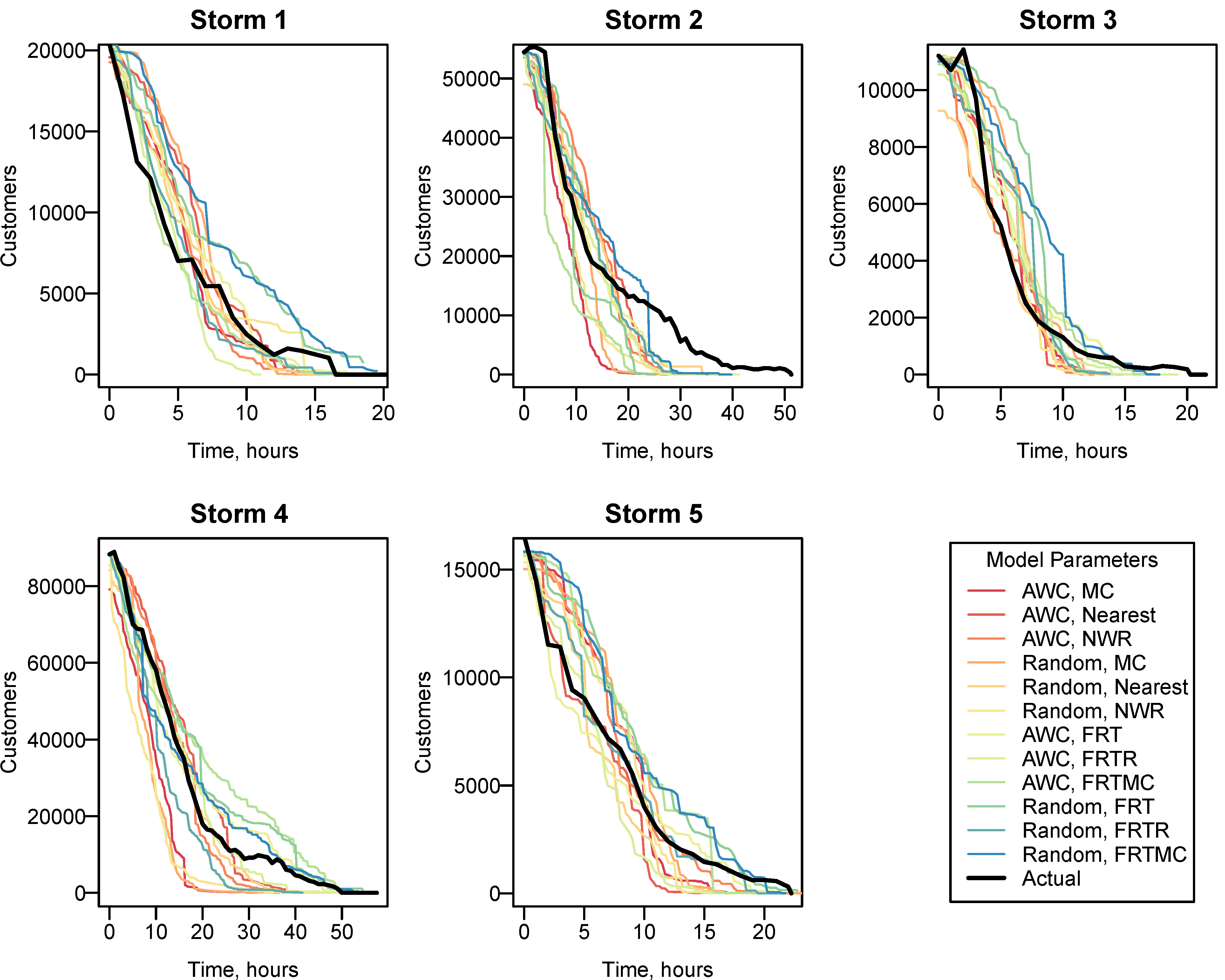
Figure 2. Outage repair time ranges were optimized for each storm and are shown in
Table 1 and
Table 2. While all repair curves showed similar large-scale behavior, there were significant differences between combinations of search strategies and starting location. However, neither the starting location nor the search strategy showed consistent trends (
Figure 2).
Table 2 includes the R
2 value, mean absolute error (MAE) and standard deviation for the top three strategies of each storm shown in
Figure 2.
Table S1 includes all strategies of each storm. Storm 1 was best fit with crews starting at area work centers and searching for the outage with the fastest repair time and the most customers affected. Storms 2 and 3 were best fit with crews starting at area work centers and searching for the outage with the fastest repair time. Both Storms 4 and 5 were best fit with crews searching for the fastest repair time within a radius of the nearest outage but Storm 4 favored crews starting at area work centers while Storm 5 favored random crew starting locations. Optimized fits had R
2 values ranging from 0.91 to 0.99, indicating adequate fits for all scenarios.
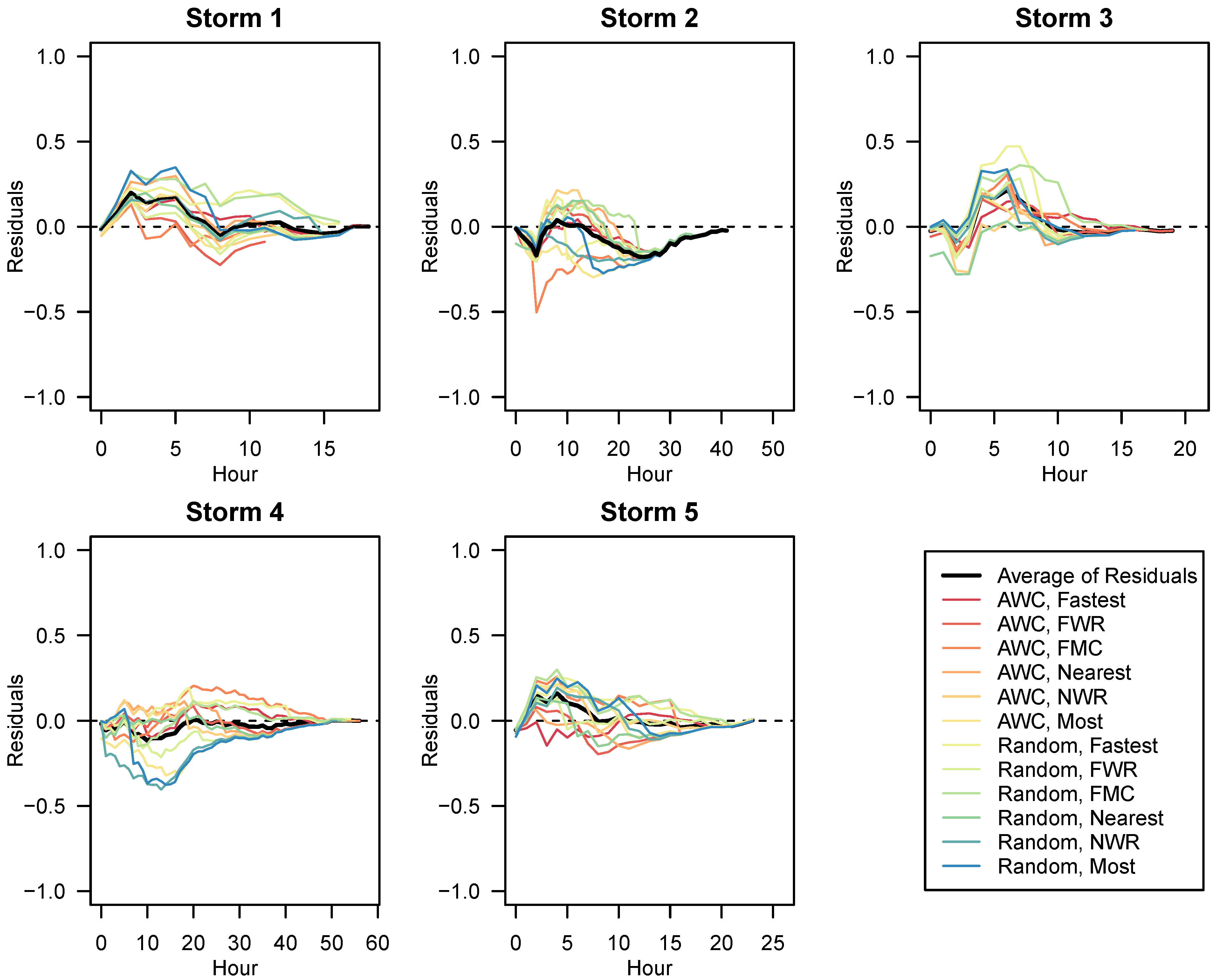
An analysis of the residuals (
Figure 3) indicates that they tend to be positive in the beginning of storms but this is not always the case. Storms 2 and 4 were larger in size and had negative residuals in the beginning meaning that they overestimated customers restored early in the storm. The early storm underestimates seen in Storms 1, 3 and 5 could be due to the fact that the model does not include priority locations such as hospitals. Utilities are aware of outages that impact the most customers and will restore these points first. Moreover, at the end of storms, there is typically a long tail representing outages that are difficult and time-consuming to repair and single service outages. The residuals in
Figure 3 have been normalized to the maximum number of customers affected per storm. The residuals were biased because they were not randomly positive and negative. Storms 1, 3 and 5 had the lowest residuals. Storms 2 and 4 have larger residuals and as seen in
Figure 3. In all cases, the residual values decrease towards zero at the end of storm recoveries.
Each storm is different in the damage it produces and therefore the length of time that repairs take on average. It is difficult to know the average repair time range of a storm before the storm occurs. As shown in
Figure 2 and
Table 2, each storm is fit with a different repair time range. These ranges were determined using the data in
Figure 4 and
Table 3.
Table 3 includes the top three R
2 value, mean absolute error (MAE) and standard deviation for each storm shown in
Figure 4. R
2 values were all >0.93.
Table S2 includes all storms and all strategies. In these simulations, crews started at random locations and searched for the nearest outage. In all cases, as the repair time range was increased starting at one hour, the MAE decreases as the R
2 value increases until the combination of highest R
2 and lowest MAE is reached. Storm 1 appeared to match well with a lower maximum repair time early in the restoration but a longer repair time later on. Storms 2 and 4 best fit to a 13 h maximum repair time and were both larger storms in this data set with 1399 and 2056 outages respectively. Storms 1 and 5 were similar in size (657 and 661 outages) but the best fitting repair time was 7 h for Storm 1 and 11 h for Storm 5. The repair time range that best fits each storm depends on more than storm size alone. Storms 1, 3 and 5 had similar number of total crews working with 201, 212 and 190, respectively. Storm 2 had 365 and Storm 4 had 392. The larger storms had more crews working, yet still had the longer repair time range.
3.1. Model Sensitivity
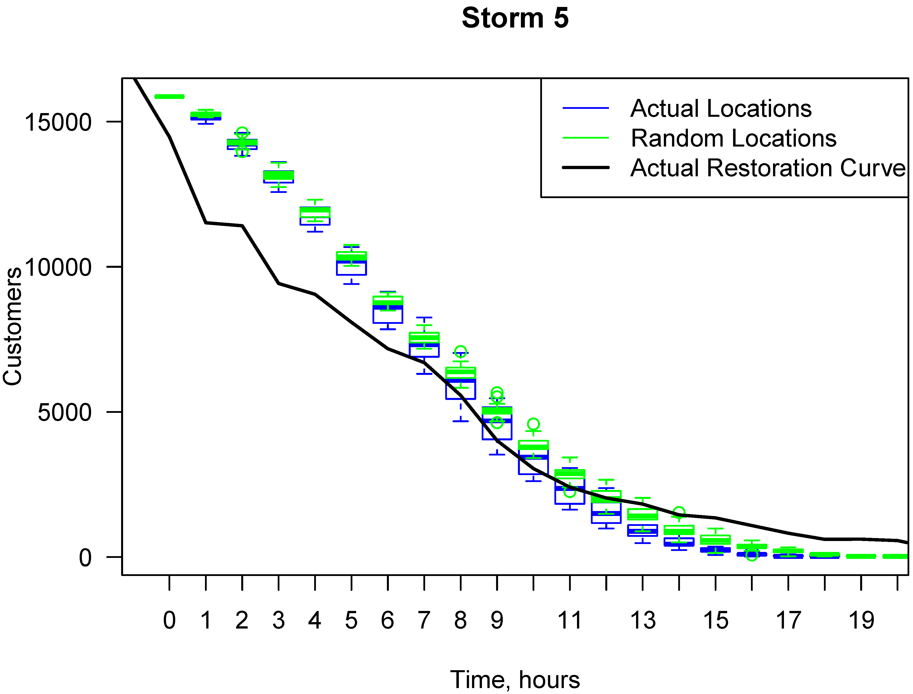
With a reasonably validated model, we next tested the sensitivity of the model to outage locations. The model was run first using the known outage locations of historic storms. It was run again using the same number of outages but randomly placed across the State of Connecticut. For consistency, the average repair time range of 1 to 10 h will be used for all subsequent What-If scenarios. As seen in
Figure 5, the two outage location options produced nearly identical results. This means that knowledge of actual outage locations is not necessary to reproduce accurate ETR curves. The model showed little sensitivity to travel speed, so the time lost to travel is negligible. Therefore, the location would have little impact on the ETR because any change due to travel distance is minor. For all storm simulations, outages will be randomly located within the state.
Tests were conducted to determine the sensitivity of the model to parameter changes. A small storm in these tests is characterized as having 1000 outages, large storms have 5000 outages and extreme storms have 15,000 outages. The number of customers affected per outage was determined by using an average from the five validation storms.
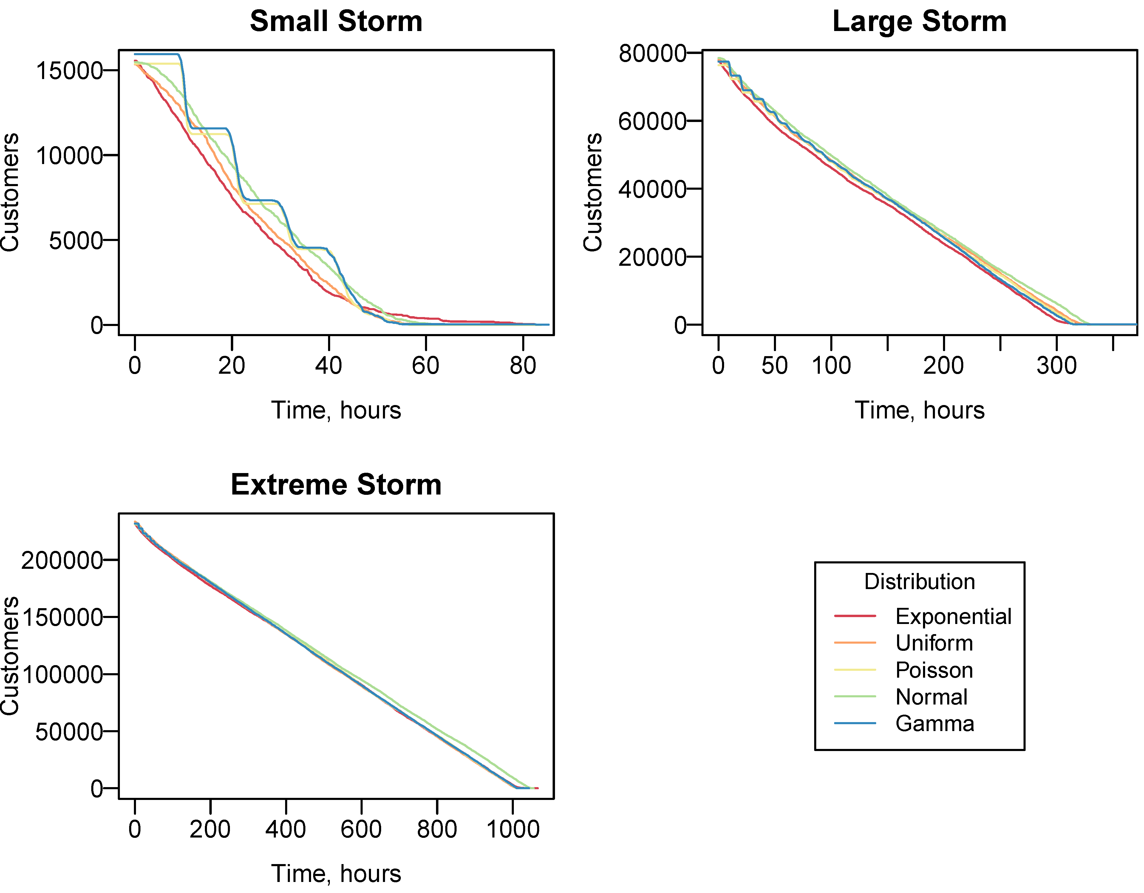
The model was tested for sensitivity to the outage repair time distribution. Previously shown results used a uniform outage repair time from 1 h until the chosen maximum repair time. However, it was unclear if different repair time distributions would lead to different overall restoration times. Storm characteristics can influence the nature of the damage caused and therefore the repair time distributions. Tested distributions included uniform, normal, exponential, gamma and Poisson and are detailed in
Table 4.
Figure 6 shows that the distribution of outage repair times has minor impacts on the final restoration time. As seen in the small storm, a gamma and Poisson distribution tends to produce a step-like restoration curve. Gamma distributions usually fit best with data with large standard deviation but the relatively low mean of the chosen repair times limits a large range. In the case a negative repair time was chosen, the model picks a new repair time. When all outages have the same repair time a step-like curve is produced because the crews arrive to their outage at similar times and are all working for the same duration. These steps become less defined over the course of the restoration process.
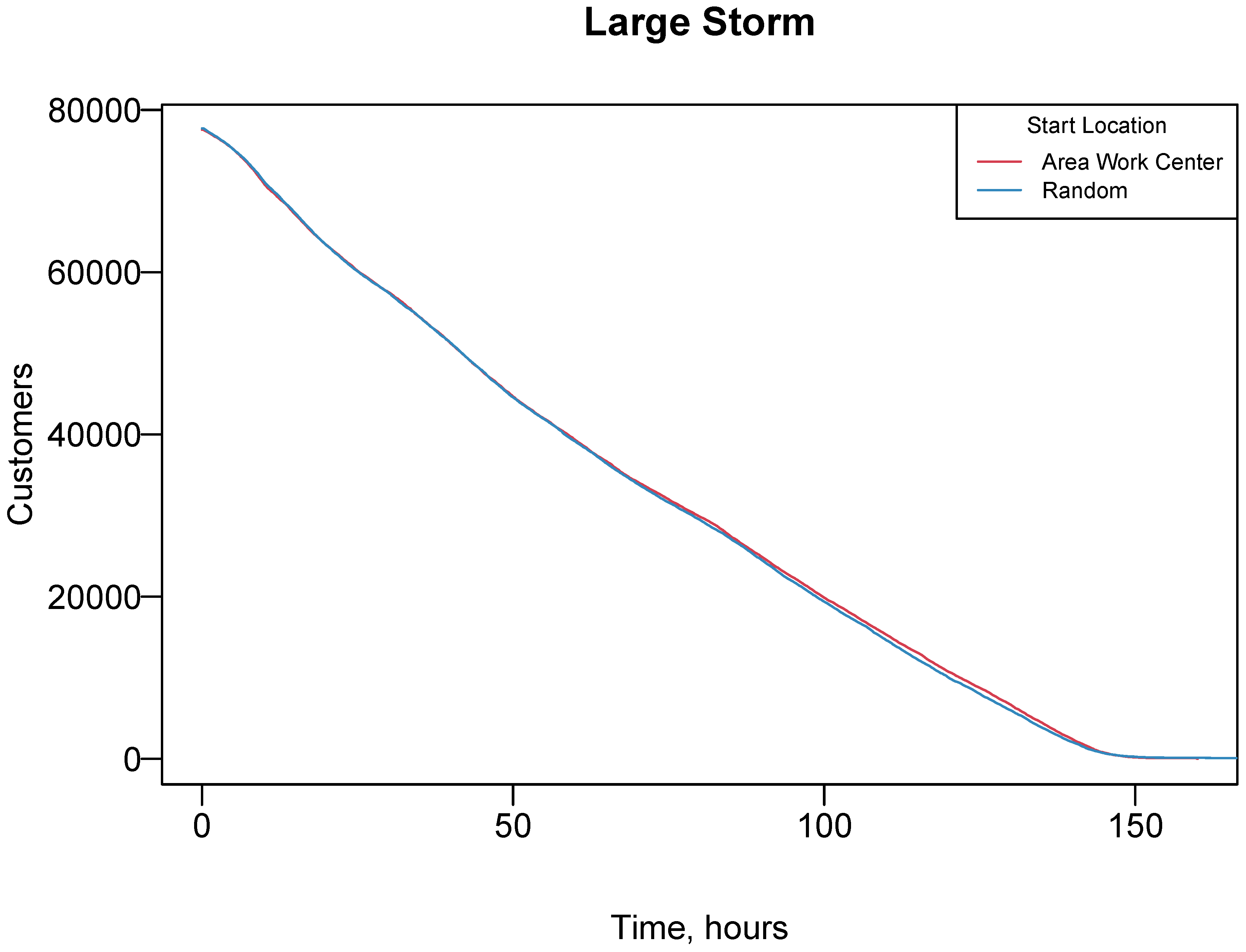
The next test compared the initial starting location of work crews for each size storm. At the beginning of the storm, crews could start at either area work centers or random locations. For this test crews would search for the nearest outage. Travel speed was set to 25 miles per hour, the repair time range was 1 to 10 h and 272 crews were working (the average number from the validated storms).
Figure 7 shows that there was little difference between the two starting location options. All future storms will be run with crews starting at area work centers, which is more realistic.
As seen towards the end of the storm in
Figure 7, some of the model runs can result in a long tail until complete restoration. This occurs when the last few outages have long repair times and when there are many single service outages. These long tails also can occur as difficult or hard to reach repairs are often left until the end. To highlight the major scenario differences, all ETR curves will be cropped when the number of customers remaining without power was no more than 20 for the small storm and 100 for the large and extreme storms.
Figures S1–S3 for small and extreme storms can be found in the
Supplementary Materials.
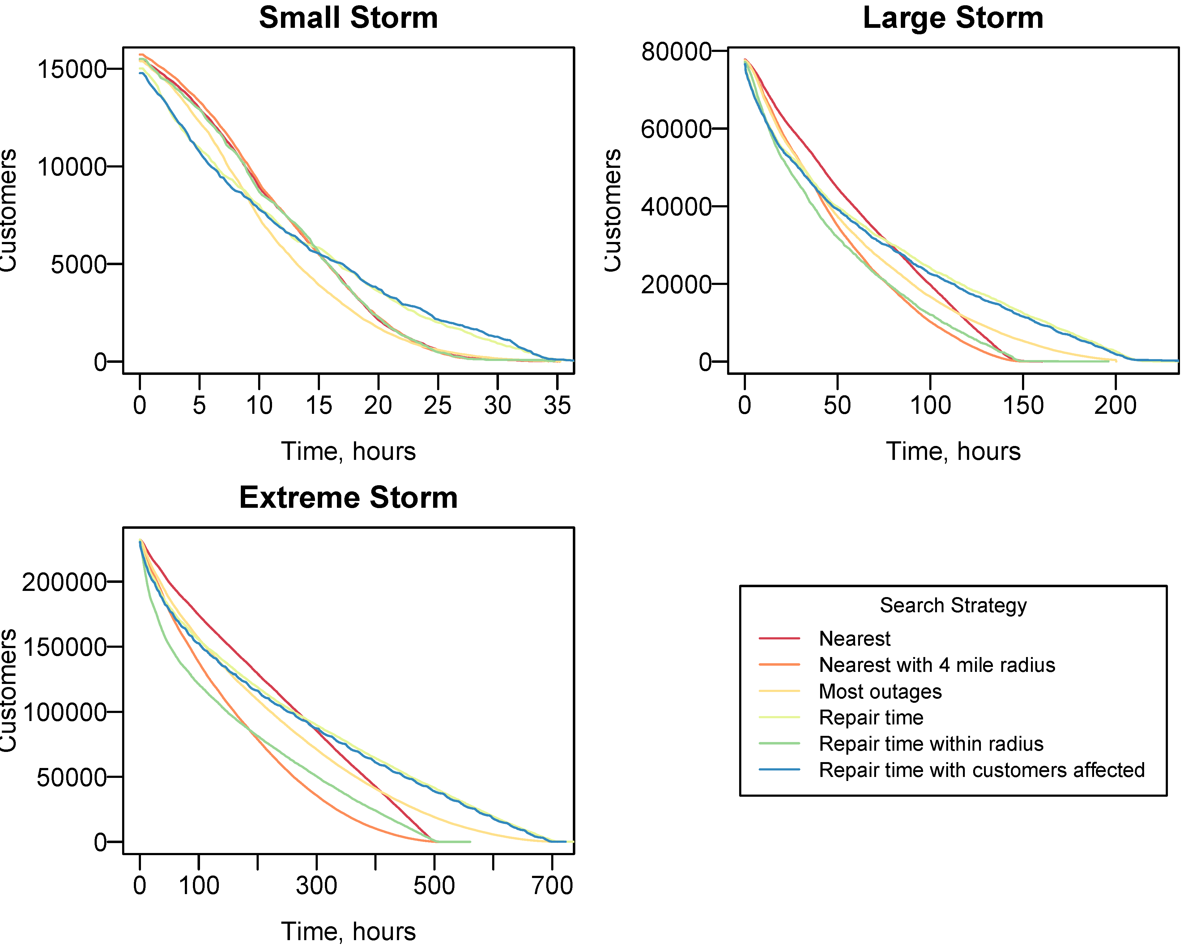
Next, the crew search strategy was varied between nearest outage, the outage with the most customers affected within a radius of the nearest outage (nearest within radius), the outage with the most customers affected, the outage with the fastest repair time, the outage with the fastest repair time within a radius of the nearest outage and the outage with the fastest repair time and most customers affected. All of the parameters were kept the same as previously described and crews started at area work centers. The radius was set to four miles for the nearest within radius and fastest within radius search options.
Figure 8 shows some sensitivity to search strategy, especially in the large and extreme storms. For the small storm, there was little difference between the nearest outage, nearest with radius and fastest repair time. The most customers affected option performed better in the beginning but a longer tail at the end lengthened the final ETR. The large storm shows a bigger difference between the nearest outage and nearest with radius options. However, the nearest within radius performed similar to the most outages option in the beginning but ended faster than most outages. The nearest and nearest within radius search strategies had similar ETRs for the large storm but nearest within radius always had less customers still without power than nearest. The biggest differences between search options came in the extreme storm situation. The nearest within radius option performed best throughout the run. In the beginning of the simulation most outages performed between nearest within radius option and nearest outage, until about the 400-h point. After the 400-h mark, the most outages option reduced the number of customers affected most slowly. The nearest within radius option reduced the number of customers affected the fastest and had an ETR closest to the nearest search strategy. In both the large and extreme storms, the search strategies using repair times have similar impacts on the ETR curves. Both fastest repair time and fastest with most customers have the longest final ETR. The fastest within radius performs the best in the beginning of the storm but then has a final ETR similar to the nearest and nearest with radius strategies. The final ETR for each search strategy and storm size can be seen in
Table 5.
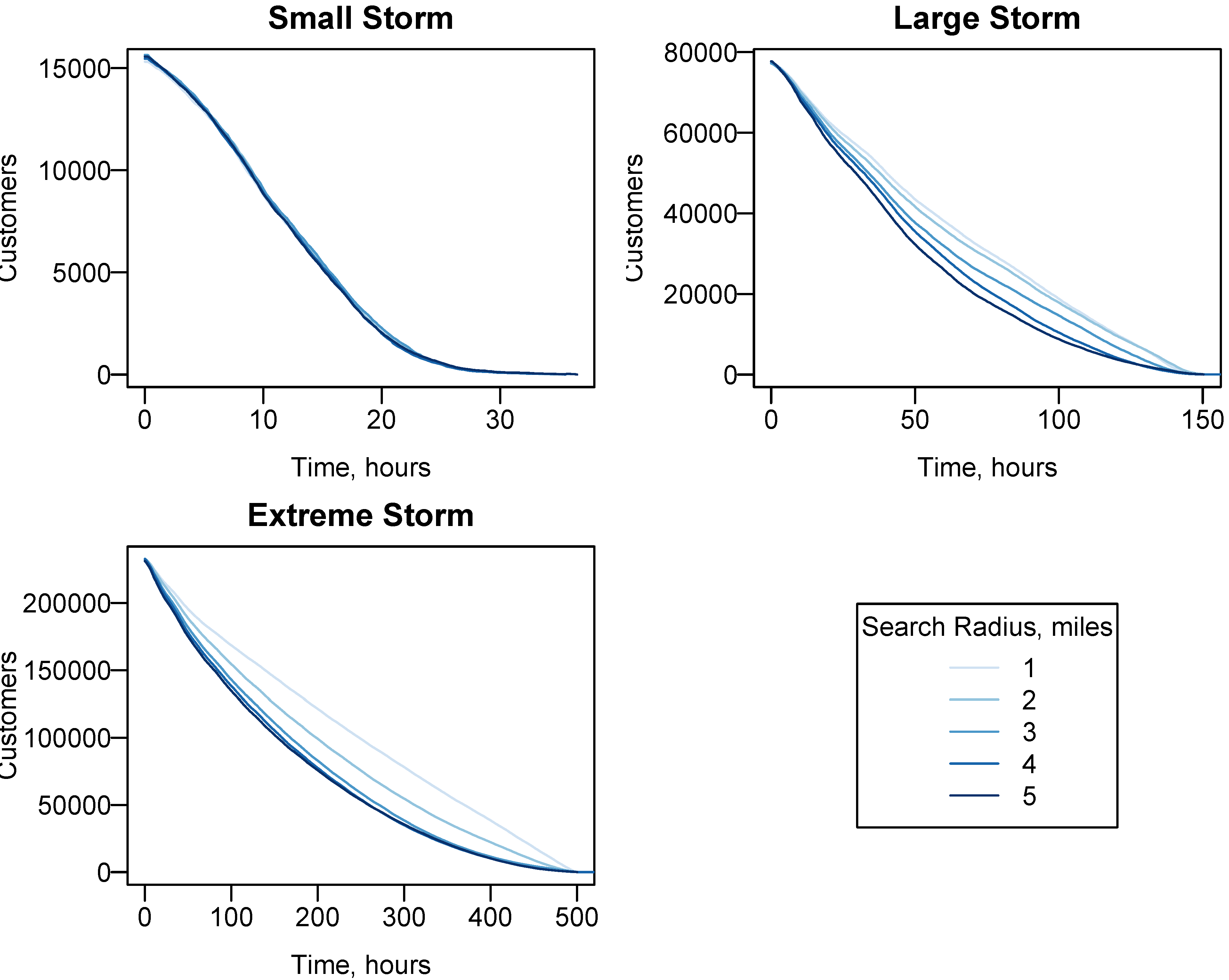
As previously stated, a four-mile radius was used for the nearest within-radius search option. Next, this radius was varied from one mile to five miles.
Figure 9 shows that the impact of the change in radius depends on the storm size and
Table 6 shows the time to restoration in days for each storm size and radius. The small storm was not sensitive to the radius, which confirms from
Figure 8 that there was little performance difference between the nearest outage option and nearest with radius option. However, the large and extreme storms were both sensitive to search radius. In both cases, a larger radius reduced the customers without power the quickest. However, the five-mile radius did have the longest tail in both the large and extreme storm.
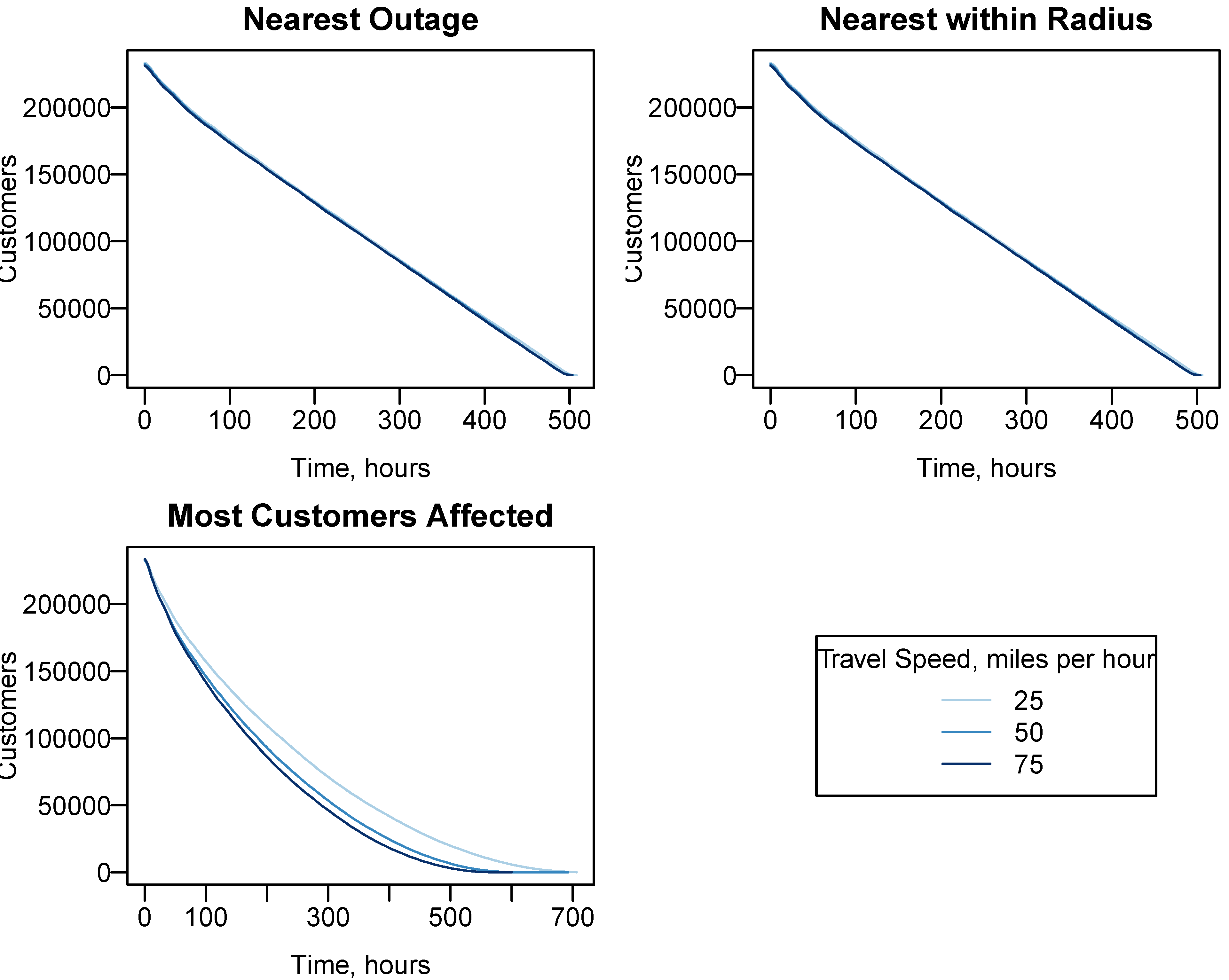
Next the model was tested for sensitivity to travel speed. The crew travel speed has little impact on the ETR, as shown in
Figure 10 for the large storms with 5000 outages and with the nearest outage and nearest within radius search strategy. However, there are slight differences in the 25 mph, 50 mph and 75 mph speeds for most outages search strategy. Repeating for the small and extreme storms yielded similar result. The small storm was not run for the nearest with radius strategy because previous tests showed it did not vary from the nearest strategy.
Figures S1–S3 for the small and extreme storm can be seen in the
Supplementary Materials. The biggest difference for all three storms was between the 25 mph and 50 mph speeds for the most outages search strategy. Increasing from 50 mph to 75 mph further reduced the ETR but not as much as 25 to 50 mph. For all three storms, the different travel speeds did not significantly alter the final restoration time.
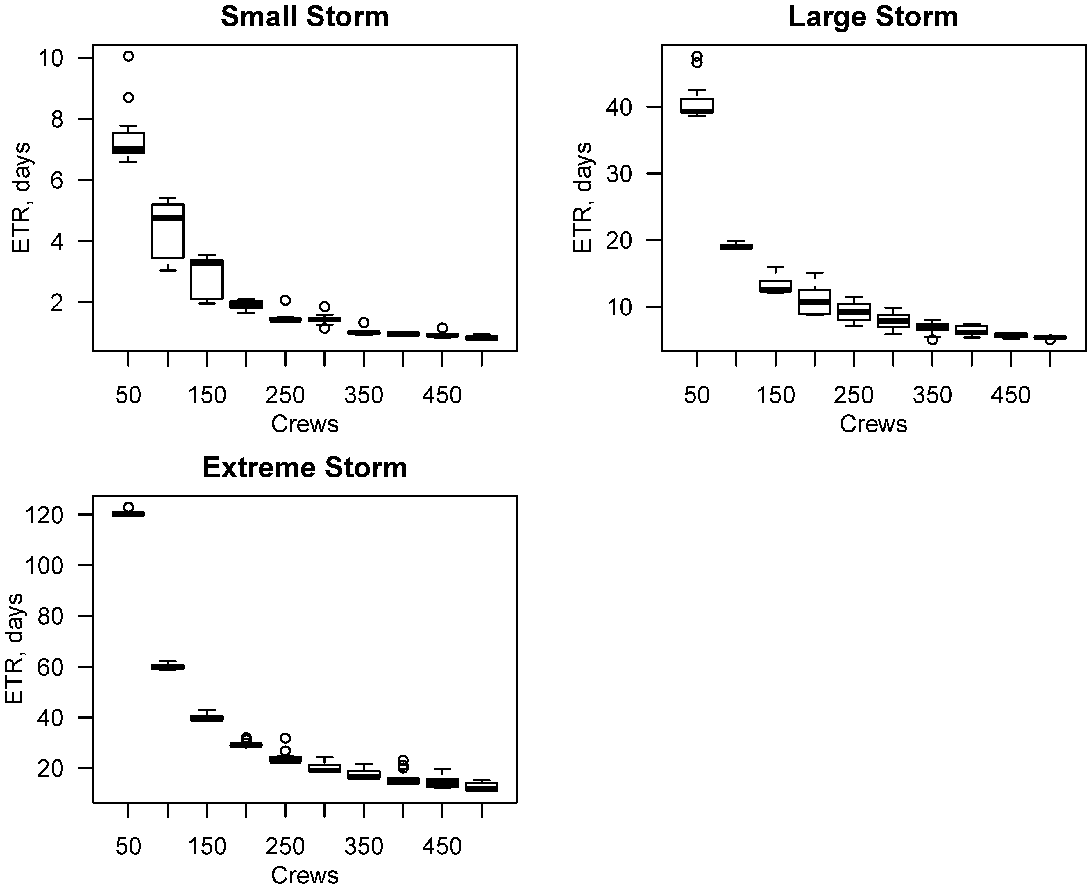
The next test varied the number of crews, as shown in
Figure 11. For each storm size, initially increasing the number of crews creates a decrease in the ETR. However, there is a threshold where bringing in more crews will have less of an impact on the ETR. For the small storm, this occurred around 250 crews and for the extreme storm it was somewhere between 400 to 450 crews.
Table 7 shows the time to restoration of each storm size based on number of crews from
Figure 11.
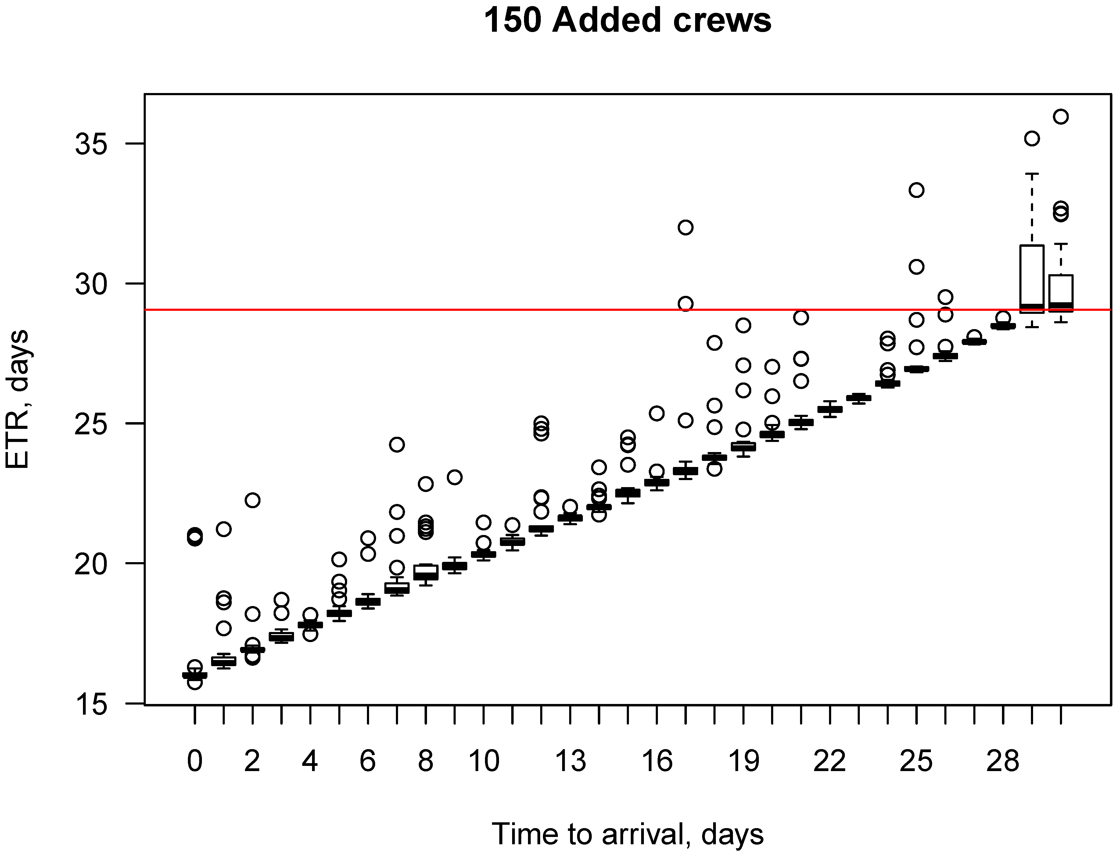
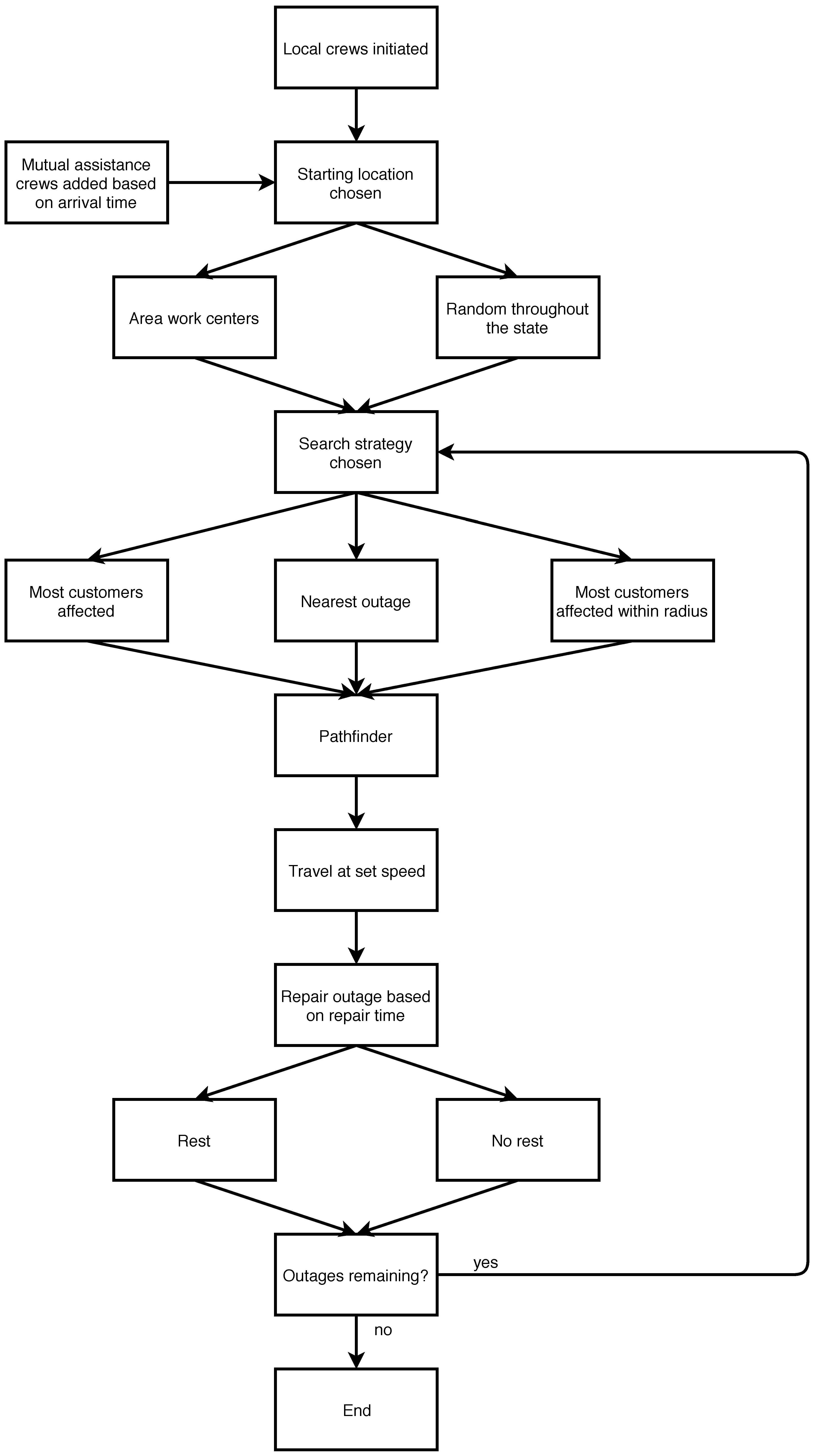
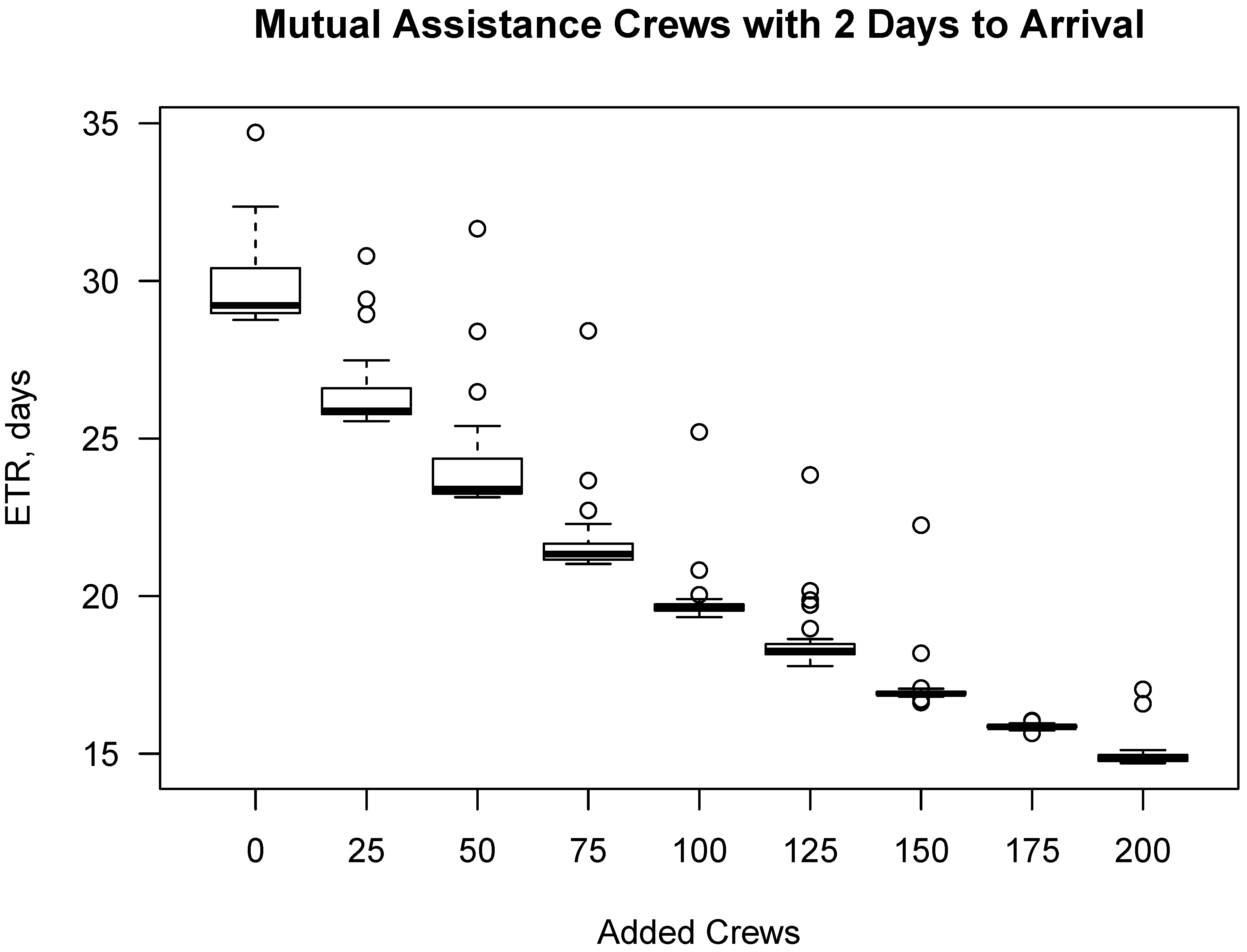
As previously mentioned, for storms with a lot of predicted outages, utility companies will call in mutual assistance crews to aid in the recovery process. This test looked at the impact on the ETR of bringing in mutual assistance crews at different times throughout the storm. First, only the time to arrival of 150 mutual crews added to 200 initial crews was varied as shown in
Figure 12 for the extreme storm only. The ETR increases with increasing time for arrival. Next, the number of crews added to 200 initial crews with a two-day arrival was varied as shown in
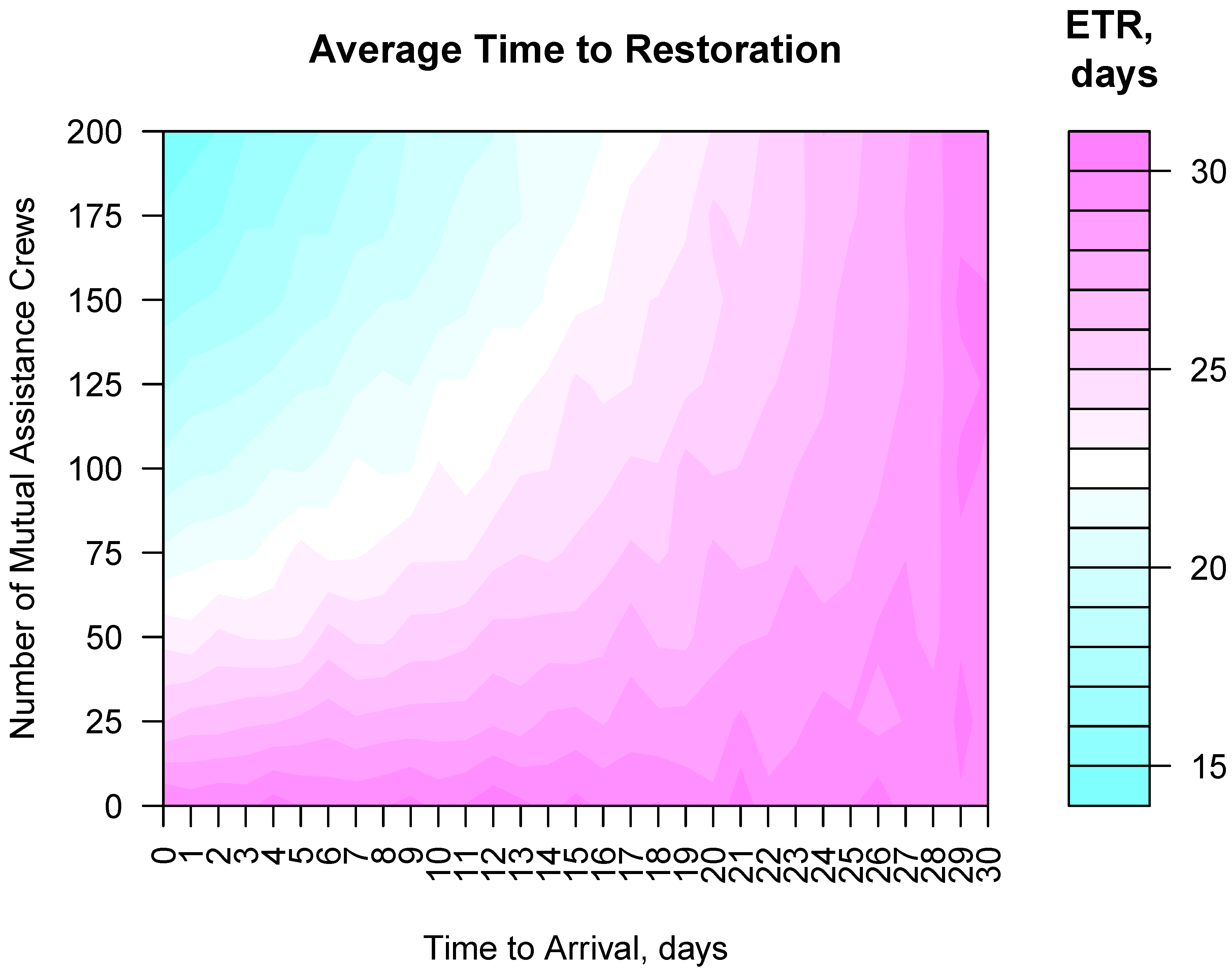
Figure 13. The ETR decreases with increasing number of added crews. Lastly, both the number of mutual assistance crews and the time to arrival was varied as shown in
Figure 14. Also, as expected, the more crews and faster time to arrival decreased the ETR while less crews and longer time to arrival increased the ETR. There was also a point where calling in more crews that would take longer to get there made less of an impact in the ETR than calling in less crews that could arrive sooner. Towards the end of a storm there are less outages to repair. If a large number of mutual assistance crews arrive later in the recovery process, there may be more crews than outages or the cost of the added crews may not justify calling them in.
3.2. Model Limitations
The goal of an ABM was to develop the simplest, yet accurate model possible. In order to accomplish this, two simplifications were made. First, Dijkstra’s algorithm does not account for power flow considerations on the utility lines. The model does not prevent multiple crews from working on the same line. Secondly, the model does not account for different work rates of regular utility crews versus mutual assistance crews or a change in work rate as the restoration process continues. Typically, mutual assistance crews will have slower repair times because they are not familiar with the system or they take longer to navigate to the outage. The model does not account for this and uses the same repair time range for regular utility crews and mutual assistance crews. As mentioned in
Figure 3, the beginning of the storm typically fits better to lower repair time ranges but the end of the storm fits better to longer repair time ranges, indicating a change in repair rates throughout a storm. In the beginning of the storm there are more resources available and towards the end of the storm the resources are less readily available.
There are several parameters where small changes in the value can result in large differences in the ETR. As shown in
Figure 4, the repair time range assigned to the outages has the biggest impact on the ETR but it is also the most variable input parameter in the model. However,
Figure 6 shows the model is insensitive to whether normal, gamma, exponential, Poisson or uniform distributions were used to assign outage repair times. Although storms can be divided into categories such as snow, ice, wind, rain and so forth, the repair time range of the outages can vary from storm to storm. Different failure types can take different times to repair, as well as different number of crews available. The ABM only assigns one crew to each outage and does not differentiate between outage types but increasing the repair time range can account for losing multiple crews to one outage. The model also does not differentiate between different crew types. In a utility company, crews are equipped for specific types of repairs. Some outages will require two or more crews to each work on their specific task.
The number of crews working and both the number and arrival time of mutual assistance crews can vary throughout a storm. The model simplified these changes for the number of crews by having a percentage of the total crews “resting.” The crews did not leave the model but did not contribute to the restoration process during that time. During storm recovery, mutual assistance crews can arrive at different times and in different groups. To allow the user to easily input any mutual aid crews, all crews enter the model at the same time.


