Article

Prediction of Concrete Arch Dam Response Using Locally Estimated Scatterplot Smoothing

1
Institute of Water and Environmental Engineering (IIAMA), Universitat Politècnica de València, 46022 Valencia, Spain
2
Canal de Isabel II, 28003 Madrid, Spain
*
Author to whom correspondence should be addressed.
Infrastructures 2026, 11(1), 9; https://doi.org/10.3390/infrastructures11010009 (registering DOI)
Submission received: 1 December 2025 / Revised: 17 December 2025 / Accepted: 21 December 2025 / Published: 23 December 2025
(This article belongs to the Section Infrastructures and Structural Engineering)

Abstract

In this research, a novel hybrid methodology is proposed for predicting the structural response of high concrete arch dams, combining the Discrete Element Method (DEM) with the Locally Estimated Scatterplot Smoothing (LOESS) technique. A structured calibration strategy is employed during the numerical model preparation to enable the generation of a wide range of reliable output variables for training and prediction. The methodology is then applied to the El Atazar arch dam to demonstrate its capability to forecast displacement and stress responses. The study reveals that using the current air temperature as an input variable is not adequate for representing the thermal behavior of the dam body; instead, the mean air temperature over a specified period yields significantly better results. Additionally, the findings highlight the importance of the loading path and the dam’s initial state in determining its structural response. The developed model shows a strong agreement between predicted and observed data, demonstrating its effectiveness in capturing the nonlinear behavior of high concrete arch dams. Compared to traditional parametric models commonly used for dam deformation analysis, the proposed framework offers greater flexibility in representing nonlinearity while requiring less training data, making it ideal for dams with limited monitoring records, such as older dams or newly operated ones.

1. Introduction

The safety evaluation of arch dams, as essential components of infrastructures, is crucial due to the severe consequences of the dams’ failure on lives, the economy, and the environment. Modern dam surveillance relies increasingly on real-time monitoring systems to provide continuous information about the dam’s current condition [1,2,3]. In addition to traditional instrumentation, advanced vision-based techniques—such as satellite monitoring and event-camera approaches—are emerging as powerful non-contact tools for detecting subtle movements, vibrations, or surface anomalies with high temporal resolution. These technologies may complement classical monitoring systems by offering richer and more flexible data streams for health assessment [4,5].
While real-time safety monitoring provides valuable information about a dam’s current condition, predicting its behavior enables proactive decision-making for future scenarios, optimizing maintenance strategies, and enhancing overall dam safety [6,7,8,9,10]. Traditionally, prediction analyses were limited to the design phase, where the stress-deformation response of the dam-foundation system was estimated before construction. Over time, numerical models (e.g., finite element models) have been developed to better understand dam behavior under current loading conditions or hypothetical future scenarios. However, in modern dam safety assessments, aided by technological advancements and increased data availability, artificial intelligence (AI) and machine learning (ML) are playing an increasingly significant role in dam engineering [11]. This approach involves developing algorithms and mathematical models that learn from historical data and sometimes incorporate predefined physics rules to simulate human intelligence, thereby enhancing efficiency by significantly reducing the time, expenses, errors, and overlooked aspects involved in human assessments [12,13]. ML-based algorithms can be applied across a broad range of dam engineering tasks, such as design optimization [14,15,16,17,18], hazard and anomaly detection [19,20,21,22,23], decision-making in operation and maintenance [6,7,8], uncertainty quantification [24], reliability and risk assessment [25], safety evaluation, and structural response prediction [26,27,28,29].
Over the last decade, numerous studies have focused on predicting the response of concrete dams. Lin et al. [30] used Optimized Sparse Bayesian learning for deformation and seepage prediction of concrete arch dams. Zhang et al. [31] adopted a surrogate model based on the multi-layer perceptron algorithm to replace the finite element calculations. Wei et al. [32] combined the Support Vector Machine with Artificial Bee Colony Optimization to monitor the displacement of a concrete gravity dam. Tao et al. [33] introduced a methodology by mixing Convolutional Neural Networks, Long Short-Term Memory, Improved Particle Swarm Optimization, and Swarm Information Entropy for stress prediction of an RCC dam based on the dam’s monitoring data. Meta et al. [34] applied a Density-Based Spatial Clustering formulation that could model relative movements between blocks of gravity dams, considering the evolution of the records over time. He et al. [35] developed a theoretical model for simulating arch dams’ foundation unloading relaxation zones. Wang et al. [36] introduced a hydraulic exponential thermal time model for hydraulic and thermal displacements of the Jinping I arch dam. Detailed research on the role of artificial intelligence and digital technologies in dam engineering can be found in [37].
Several researchers have focused on the displacement prediction of concrete arch dams using a hybrid approach. A selection of recent studies is presented in Table 1. Within these hybrid frameworks, some studies rely on hydrostatic-thermal-time (HTT) models or their variations, including hydrostatic-seasonal-time (HST), hydrostatic-seasonal-time-thermal (HSTT), and hydrostatic-hysteretic-seasonal-time (HHST) models. These models establish regression-based relationships between input variables (such as water level and air temperature) and output parameters (typically dam body displacements). It usually relies on a fixed regression formulation with constant coefficients.
This article proposes a hybrid approach that combines the Discrete Element Model (DEM) and the Locally Estimated Scatterplot Smoothing (LOESS) technique to predict the response of concrete arch dams. The methodology is then applied to the El Atazar concrete arch dam to demonstrate its effectiveness. Key advantages and innovations of this research are as follows:
  • A detailed strategy is proposed for the thermo-mechanical calibration of numerical models for high concrete arch dams.
  • Instead of using parametric regression models—which apply a single regression function across the entire dataset—this study employs a nonparametric regression approach that dynamically defines the regression function for each individual input. This adaptability enables the capture of highly nonlinear dam behavior without relying on excessively complex machine learning models.
  • The training dataset is generated entirely from a well-calibrated numerical model, eliminating the influence of noisy or invalid measurements often present in field observations. This ensures more reliable and robust predictions. However, an optional mechanism can be included to integrate new instrumentation data when needed, allowing for model correction over time.
  • Since training data is derived from the numerical model, the methodology can predict multiple response types, including deformation, stress, and joint opening. In this study, stress and deformation are selected to demonstrate the applicability of the methodology.
  • The input variables include reservoir water elevation and air temperature. However, instead of using the current air temperature, a study is conducted to identify a more effective temperature-based variable for improved prediction accuracy.
  • Initial analyses reveal that nonlinear concrete arch dam responses depend on the loading path, i.e., two models with similar final water elevation and air temperature but different historical loading conditions show different responses. To account for this, the numerical model is evaluated under various possible loading paths, ensuring that the training dataset includes not only the actual loading history experienced by the dam but also a broader range of potential scenarios.

2. Locally Estimated Scatterplot Smoothing

Regression models can be categorized into parametric (e.g., linear and nonlinear regression) and nonparametric methods based on the metamodel type [55,56]. Nonparametric regression, also called smoothing methods, instead of relying on a predefined functional form across the whole sample domain, defines the prediction model for each individual input, as shown in Figure 1 [57]. This local approach allows it to capture local patterns more effectively than traditional parametric methods, making it particularly useful for complex, nonlinear relationships such as dam-foundation system predictions [58]. Standard nonparametric regression techniques include Kernel Regression, Locally Estimated Scatterplot Smoothing (LOESS), Regression Splines, and Decision Tree-Based Regression. Among these, LOESS is selected for this study due to its high accuracy and low computational cost [58].
For a dam-foundation system, the relationship between the output parameter Y and input variable x may be defined by:
Y = f (x)
where f(.) is a quadratically integrable function. In the LOESS model, this equation may be rewritten as [59]:
Y i = m X i + w X i ε i ,   i = 1 , ,   n
where X i , ε i , and n are the input variable vector, the independent error random variable with a mean of zero and variance of one, and the sample size, respectively. In this formula, m(.) and w(.) are conditional moments and can be defined as:
m(x) = E (Y|X = x)
w2(x) = Var (Y|X = x)
where E and Var denote the expected value and variance, respectively. Conditional expectation m(x) for z in the neighborhood of x can be approximated using a polynomial function of order p as:
m z m ¯ z = j = 0 p m j x j ! z x j j = 0 p β j z x j   =   β 0 +   β 1 z x +   β 2 ( z x ) 2 + +   β p ( z x ) p
where β j   is the regression coefficients calculated by solving the weighted least-squares problem for each x:
min β i = 1 n ( Y i j = 0 p β j ( X i x ) j ) 2 K ( X i x h )
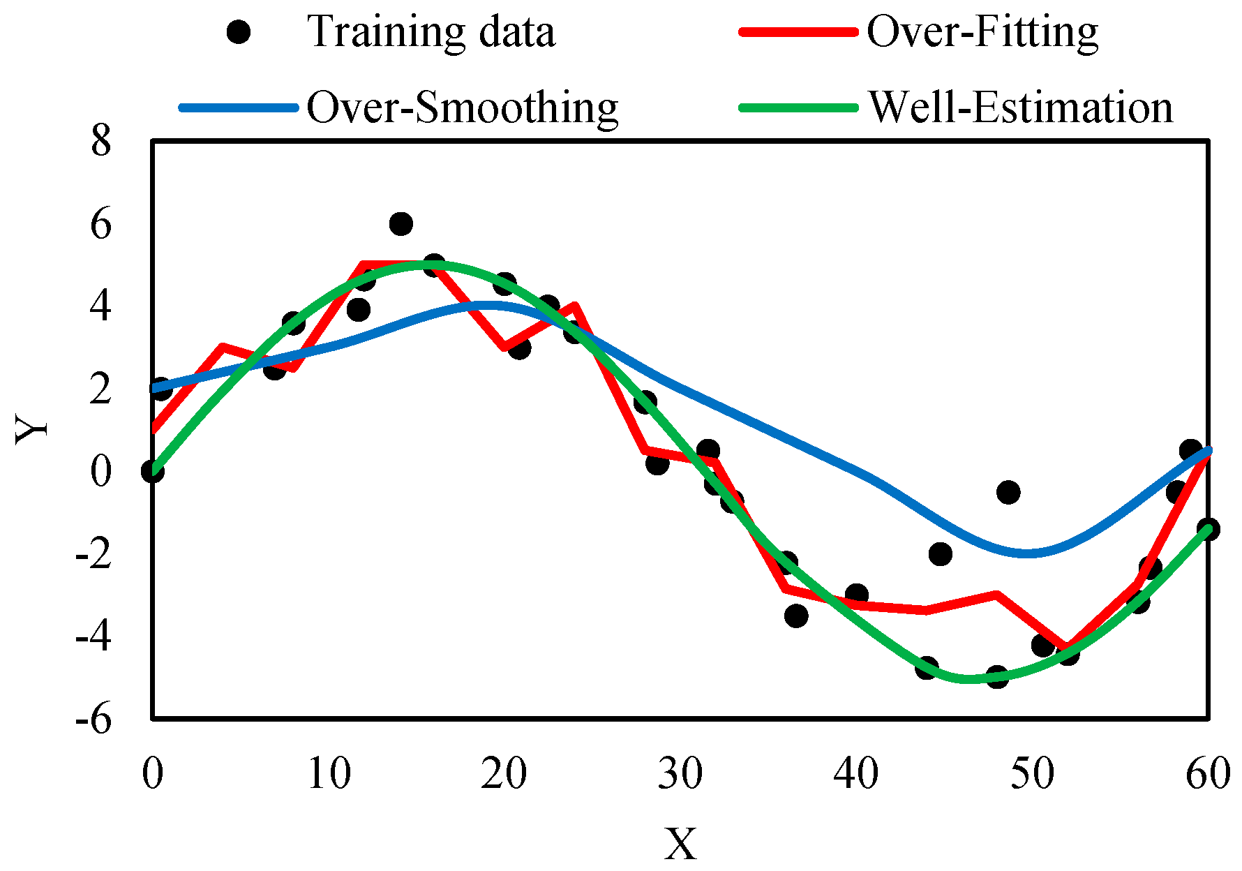
K ( . ) and h represent the Kernel function and smoothing (bandwidth) parameters, respectively. The smoothing parameter h for each x is defined as the maximum distance to the θ nearest neighbors of x. The smoothing parameter controls the complexity of the model [60]; a large smoothing parameter may over-smooth the prediction, while an extremely short one over-fits the training data, i.e., produces a high fluctuation in estimation, as shown in Figure 2 [61]. In this article, the parameter θ , which may range from 1 to n, is selected through a trial-and-error process to minimize the prediction error.
Wang and Xu [62] provided a detailed discussion on kernel function selection. In this study, the normal kernel is used for its efficiency and well-established performance as defined by the following:
K ( α ) = e x p ( 0.5 ( α ) )
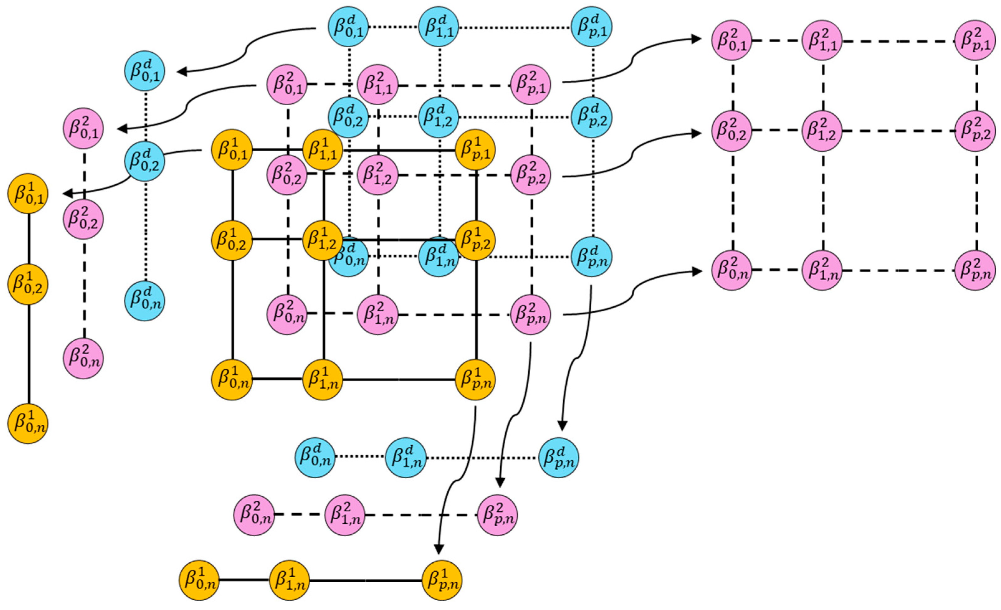
Ultimately, β will be a 3-dimensional matrix with dimensions (p + 1) × n × d, where d represents the number of independent input variables (Figure 3). β for the input variable l 1 ,   ,   d is a 2-dimensional matrix and can be estimated by:
β l = ( Q T W Q ) 1 Q T W Y T = β 0,1 l β p , 1 l β 0,2 l β p , 2 l β 0 , n l β p , n l
where
Q = X 1 x X 1 x p X 2 x X 2 x p X n x ( X n x ) p
W = d i a g K ( X i x h m )
Y = Y 1 ,   Y 2 ,   , Y n
Similarly to the function m(.), the function w2 (x) can be approximated by:
w 2 z w ¯ 2 z = E r 2 X = z = j = 0 q γ j z x j = γ 0 + γ 1 ( z x ) + γ 2 ( z x ) 2 + + γ p ( z x ) p
r 2 = ( Y m ( X ) ) 2
where q is the variance function order. γ j   , which is the regression coefficient, is calculated by solving the weighted least-squares problem for each x:
min γ i = 1 n ( r ¯ i 2 j = 0 q γ j ( X i x ) j ) 2 K ( X i x h )
r ¯ i 2 = ( Y i m ¯ ( X i ) ) 2

3. The Numerical Model

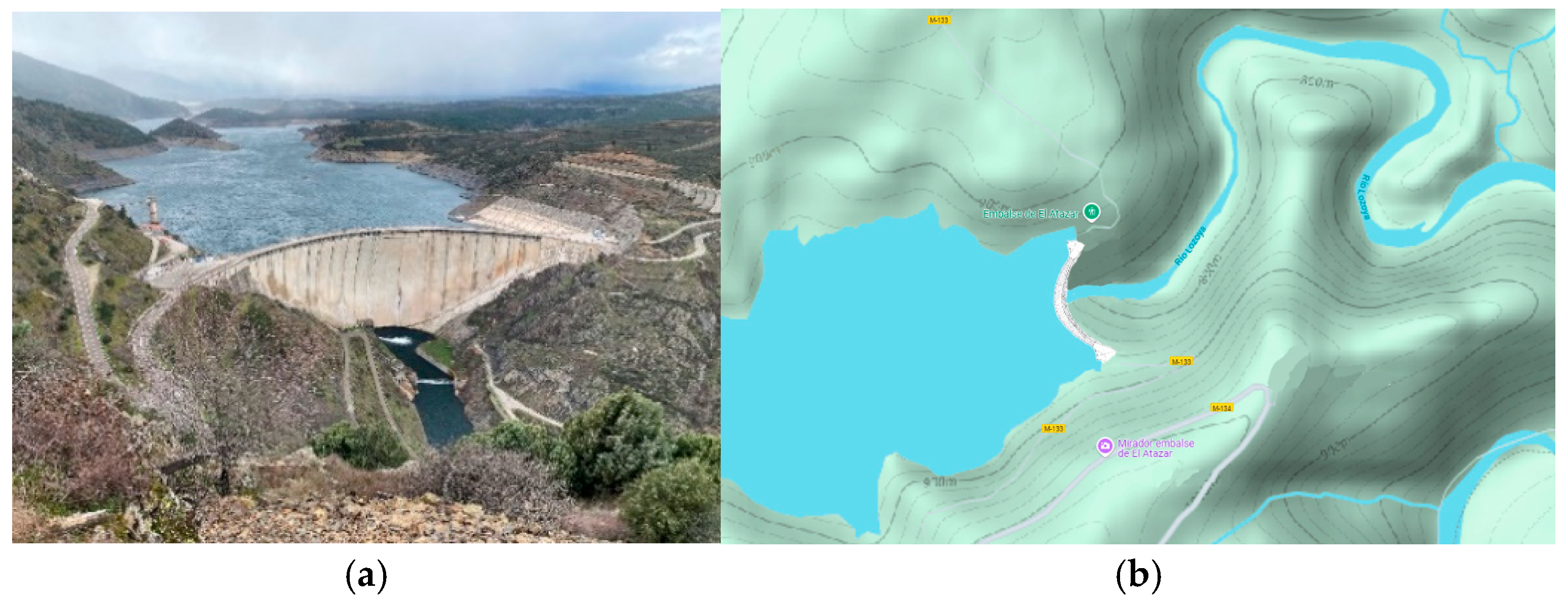
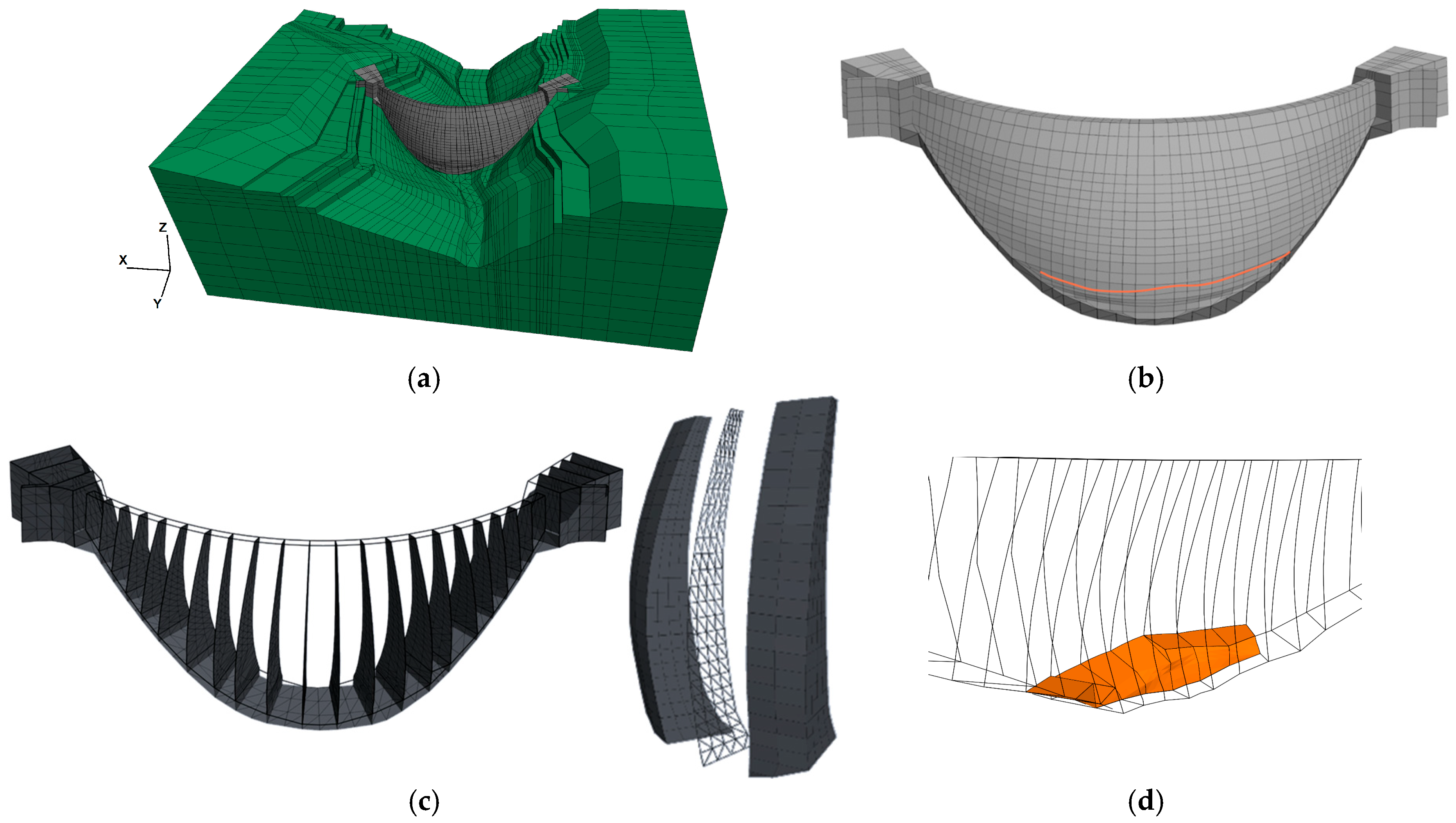
In this study, the El Atazar dam in Spain is selected as a case study (Figure 4). It is a high, thick, double-curvature concrete arch dam with a height of 141.4 m and a crest length of 484.0 m. The dam body is divided into 21 blocks with vertical contraction joints. The central cantilever thickness at the base and crest measures 36.0 m and 6.5 m, respectively [63]. Figure 5 illustrates the discrete element model of the dam and foundation developed using FLAC3D [64]. The model provides a detailed representation of the foundation layout (Figure 5a), the dam’s geometry (Figure 5b), the vertical contraction and peripheral joints (Figure 5c), and the historical injected crack surface of the dam body (Figure 5d). According to ICOLD recommendation [65], the foundation is extended at least 1.5 times the dam height in all directions. The discrete element model comprises a total of 28,306 elements and 15,337 nodes.
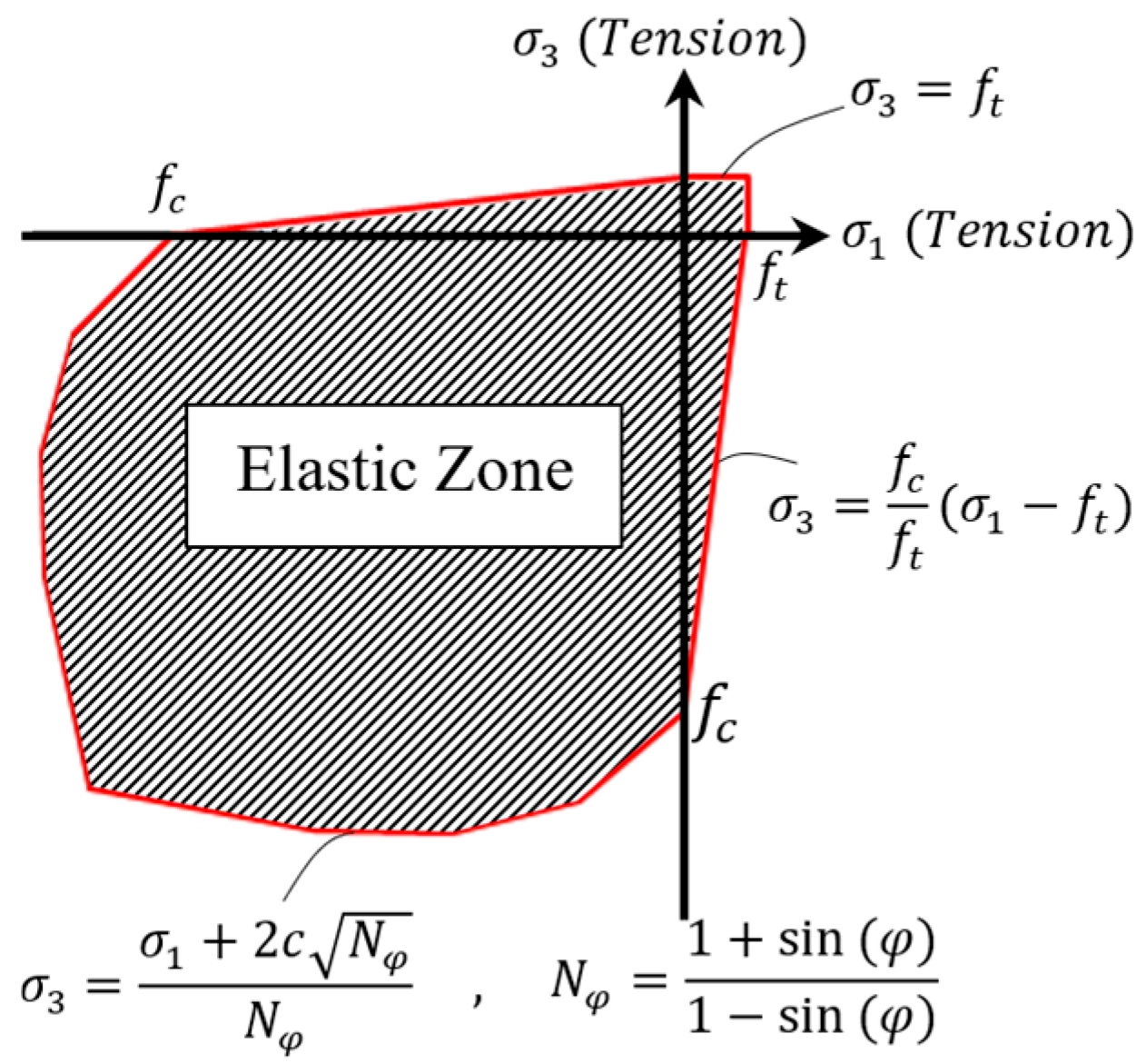
To account for material nonlinearity, the elastoplastic Mohr-Coulomb constitutive model is applied to the dam body concrete, with the corresponding yield surface illustrated in Figure 6. In this Figure, σ 1 , σ 3 , f t , f c , c , and φ are the minimum and maximum principal stress, uniaxial tensile and compressive strength, cohesion, and friction angle, respectively. The Mohr–Coulomb constitutive model was selected because it provides a robust and widely validated representation of the nonlinear elastoplastic behavior of mass concrete and rock in large dams. Its shear strength parameters (c and φ) are well supported by laboratory tests and in situ investigations, which makes the calibration process more straightforward. In this research, more advanced constitutive models—such as the Hoek–Brown or Drucker–Prager models—were intentionally avoided, as their additional parameters increase calibration complexity without necessarily improving predictive performance for the global response quantities analyzed in this work. In this context, the Mohr–Coulomb model offers an optimal balance between physical realism and computational efficiency.
However, rock mass behavior is modeled using a linear elastic approach. To simulate model discontinuities (i.e., vertical contraction joints, peripheral joints, and the injected crack surface), the interface contact element embedded in FLAC3D is utilized. This element enables elastoplastic slip and the opening of discontinuity surfaces. For more information on the shear and normal behavior of the interface elements, refer to [66,67]. The constitutive model’s parameters are determined through the calibration process, which is explained in Section 4. The movement boundary conditions are fixed displacements in the normal direction at the lateral foundation boundaries, while the base is fully constrained in all directions.
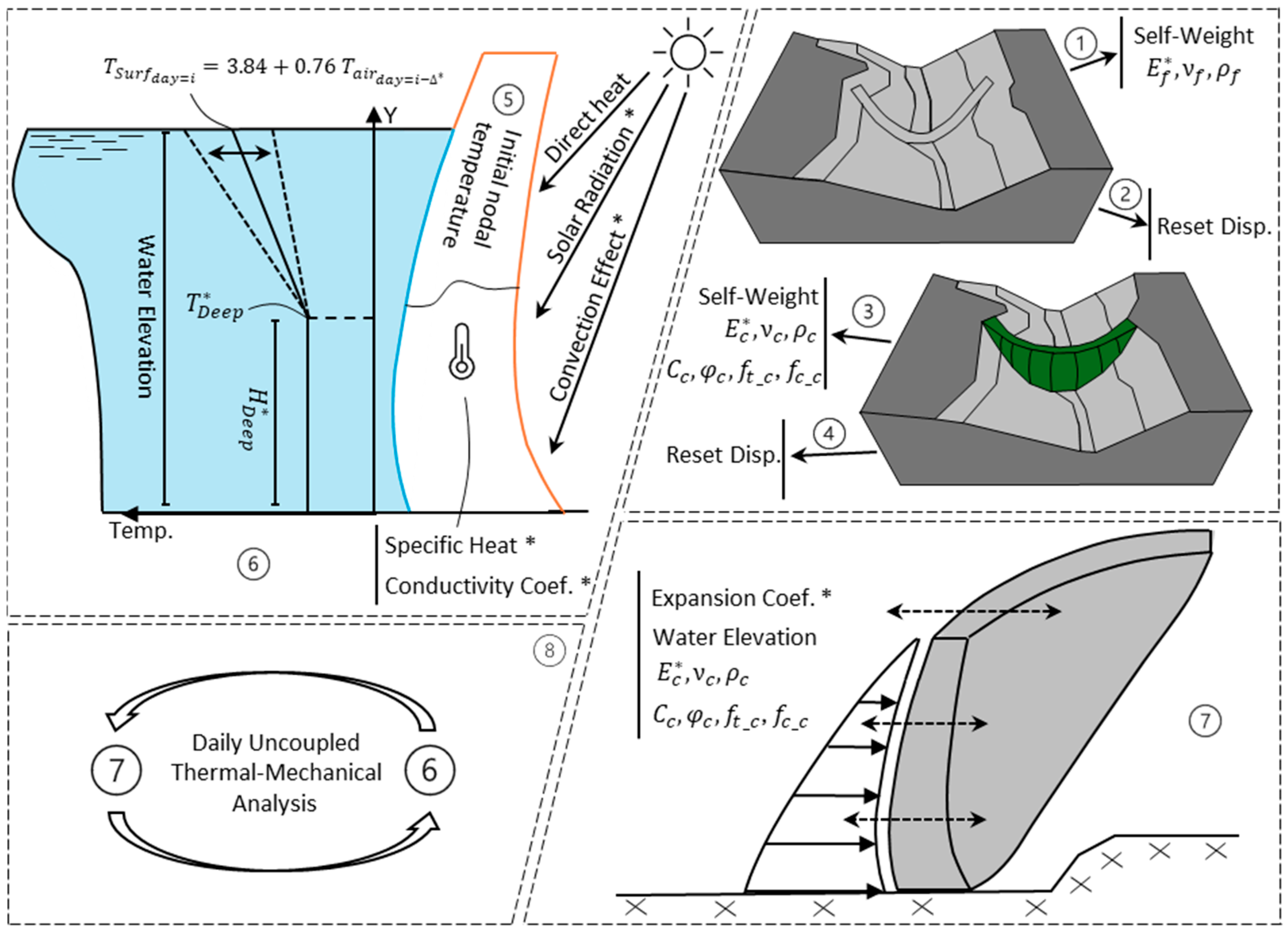
The loading process in this study follows a sequential approach, as illustrated in Figure 7.
  • Foundation Self-Weight: The foundation elements (without the dam body) are called and analyzed under their self-weight.
  • Stress Initialization: Displacements are reset to zero while retaining stresses for the next step. This allows the estimation of in situ foundation stresses.
  • Dam Self-Weight: The dam body elements are introduced, and the model is solved under the dam’s self-weight. It is worth mentioning that, in this study, the dam body stage construction is not simulated, as the primary analysis has indicated that it has a negligible impact on the stress-deformation field.
  • Displacement Reset: Similarly to Step 2, displacements are set to zero while retaining stresses. This step is essential for model calibration, as it enables comparisons between the model displacement and observed displacements from pendulum readings.
  • Initial Thermal Field Definition: The initial temperature field of the dam body is defined for each model node based on thermometer readings for day i.
  • Thermal Simulation: Thermal boundary conditions for day i + 1 are applied to the upstream and downstream faces of the dam body. These conditions are categorized as dry or wet based on whether the surface is in contact with the reservoir. The dry boundaries are influenced by the air temperature, solar radiation, and convection effects. The wet boundaries are defined by the water temperature, which varies in response to air temperature fluctuations and reservoir elevation. Further details on these boundary conditions are provided in Section 4. After applying the thermal boundary conditions, a transient uncoupled thermal analysis is performed over one day (86,400 s). In this step, the temperature variations do not induce deformations.
  • Hydrostatic Loading: The hydrostatic pressure for day i + 1 is applied to the upstream face of the dam body, and a mechanical analysis is performed to update displacements and stresses according to the new thermal and hydrostatic conditions.
  • Time Stepping: Steps 6 and 7 are iteratively repeated for the subsequent days.

4. The Numerical Model Calibration

The numerical model calibration is carried out in two stages. First, the thermal field of the dam body is calibrated by comparing the model’s nodal temperatures with thermometer data. Once the simulated temperatures closely match real temperature distributions for each day of analysis, the mechanical properties are adjusted to ensure that the model’s displacements align with pendulum measurements. The thermal calibration consists of three key components, as shown in Figure 7, Step 6:
(I)
Wet Surface Temperature Calibration: This step involves calibrating the reservoir water temperature. On any given day, the water temperature typically varies linearly from the surface water temperature to the deep-water temperature, after which it remains constant down to the dam’s base. The surface water temperature is influenced by air temperature with a certain time delay. A commonly used approach to relating surface water temperature to air temperature is Bofang’s formula [68]:
T S u r f d a y = i = 3.84 + 0.76 T a i r d a y = i
where T S u r f d a y = i , T a i r d a y = i , and represent the surface water temperature on day i, the air temperature on day i , and the delay between the maximum air and surface water temperatures, respectively. For the wet surface temperature calibration, the depth and temperature of the deep water, as well as the delay increment, are chosen as the calibration parameters.
(II)
Dry Surface Temperature Calibration: The temperature of dry surfaces is influenced by the mean daily air temperature, solar radiation, and convection effects. Solar radiation is estimated by increasing the air temperature by a specific amount. Léger et al. [69] suggested increasing the air temperature by 2 °C in summer and 5 °C in winter to approximate the solar radiation effect on the concrete dam’s surface. However, these values require calibration, as they may vary depending on geographic location, climate conditions, and surface orientation. The convection effect is incorporated into the model by a predefined convection coefficient, which also requires calibration to accurately reflect heat exchange between the dam surface and the surrounding air. Thus, the calibration parameters for dry surfaces include solar radiation temperature and convection coefficient.
(III)
Inner Nodes Temperature Calibration: The temperature of inner nodes is influenced by the upstream and downstream thermal boundary conditions, as well as the thermal properties of the dam material, specifically its specific heat capacity and thermal conductivity. These two parameters should be carefully calibrated to ensure consistency with observed temperature distributions.
The reservoir water elevation and mean daily air temperature variation for the fitting (also calibrating the numerical model) and predicting periods are presented in Figure 8. To calibrate the wet surface temperature, an inverse trial-and-error approach is employed. In this approach, an initial value is first assumed for the delay value (∆), deep-water temperature ( T D e e p ), and deep-water height ( H D e e p ). After running the numerical model, the nodal temperatures on the upstream surface of the dam body are compared with thermometer readings from the reservoir. The calibration parameters are then adjusted through an inverse trial-and-error process until the nodal temperatures in the model match the reservoir thermometer readings. Throughout this process, engineering judgment is applied to ensure that all adjustments remain within the rational parameter ranges reported in the dam project documents. The wet surface calibration results demonstrate that applying a delay of 7 days between the peak air temperature and surface water temperature, along with setting H D e e p = 88.0 m and T D e e p = 6.5 °C, yields an acceptable match between simulated and observed temperatures. Figure 9 presents a comparison for two representative days—one in summer and one in winter.
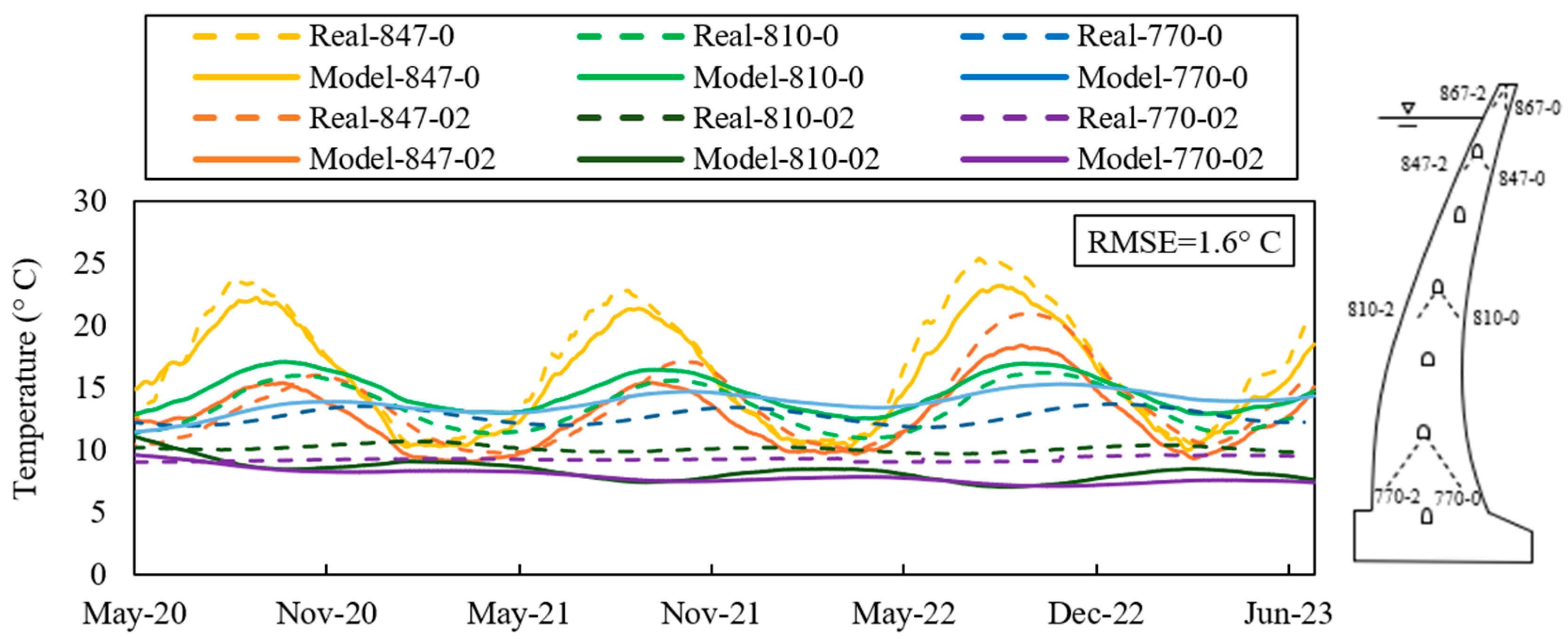
After this step, the remaining thermal calibration variables are adjusted using a similar strategy to simulate the temperature distribution on the downstream surface and within the dam body. Figure 10 illustrates a comparison between the model’s nodal temperatures and thermometer readings for the central cantilever over a period of three years (the fitting period in Figure 8), using the calibrated values listed in Table 2. The results show a good agreement between the simulated and observed temperatures, with a root mean squared error (RMSE) of 1.6 °C.
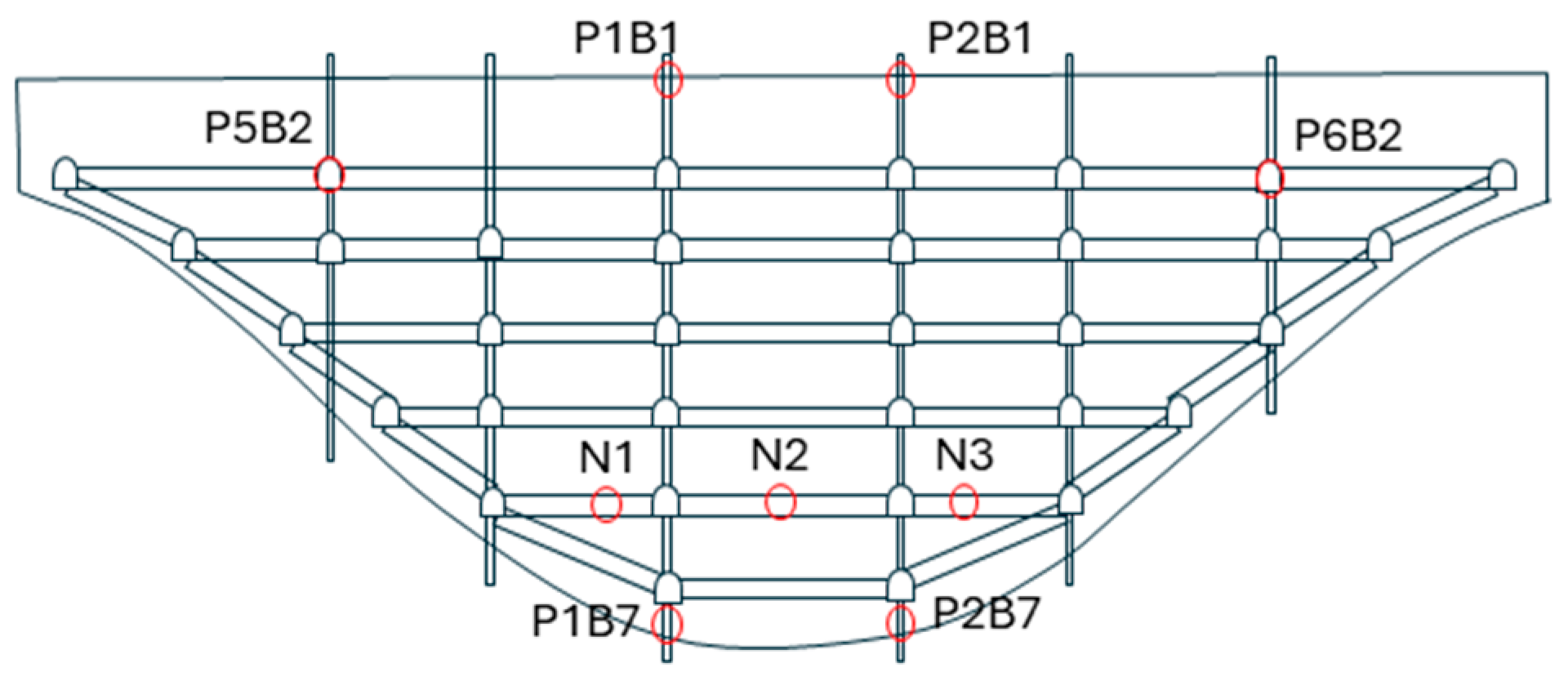
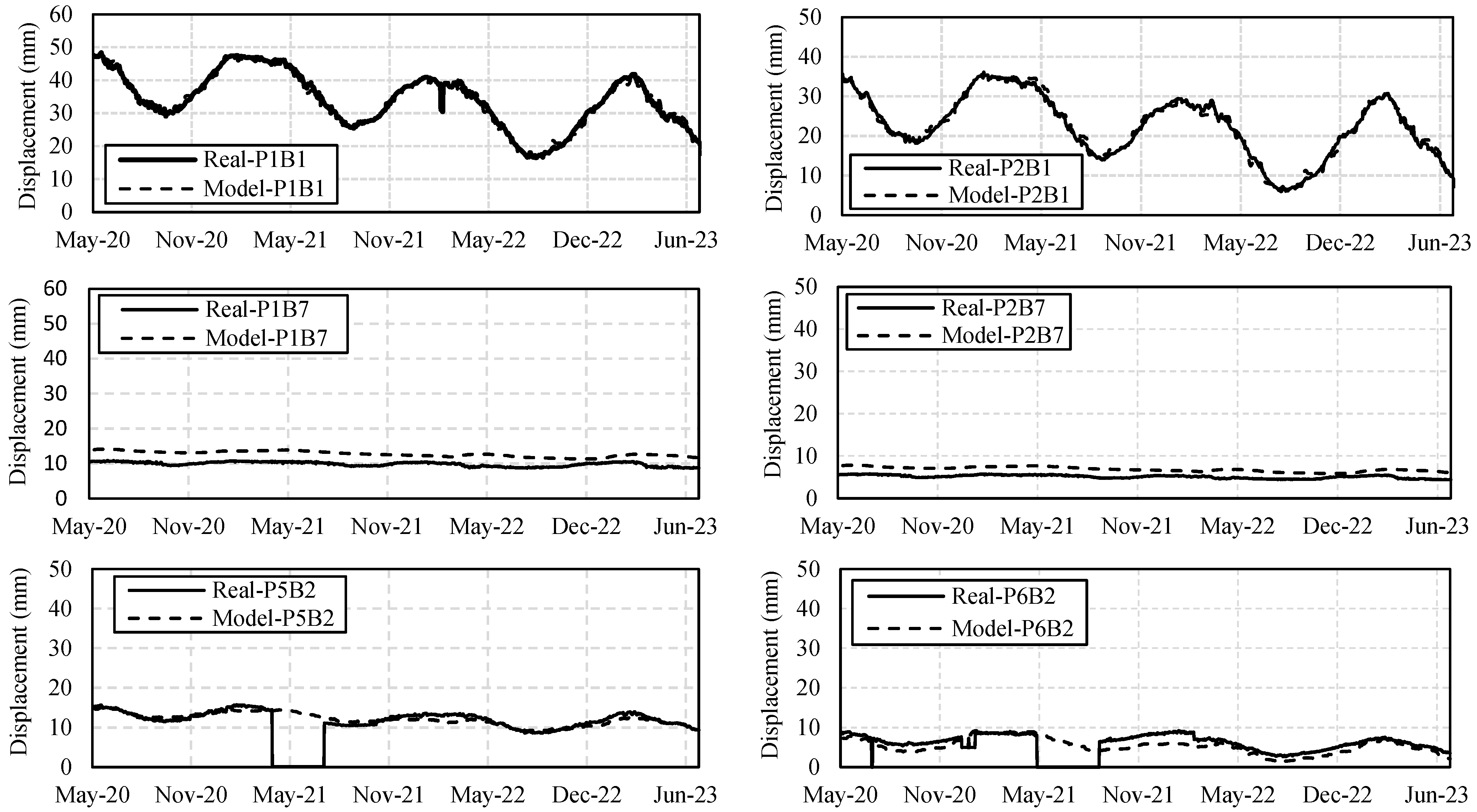
Once the temperature field within the dam body concrete is calibrated, displacement calibration is performed over a 3-year period (the fitting period in Figure 8) using a similar iterative adjustment of the mechanical properties of the dam and foundation, while ensuring that all adjustments remain within the rational parameter ranges reported in the dam project documents. The mechanical parameters selected for calibration include the elastic modulus of the concrete ( E c ), the deformation modulus of the foundation ( E f ), and the thermal expansion coefficient, and the rest are considered deterministic. These calibration parameters were chosen due to their relatively significant effect on the stress-deformation response of high concrete arch dams [70,71,72]. For the comparison, the pendulum reading points P1B1, P1B7, P2B1, P2B7, P5B2, and P6B2 are chosen (Figure 11). The final calibrated mechanical parameters are listed in Table 3. It is worth noting that two different deformation moduli are assigned to the left and right abutments to account for the greater radial movement observed in the left-side pendulums compared to those on the right. As shown in Figure 12, the numerical model is able to predict the real displacements with high precision.

5. Response Prediction Using a Hybrid Methodology

This section presents the response prediction of high concrete arch dams using a hybrid approach that combines numerical model results with the LOESS method. The methodology consists of three major steps: (1) training data preparation using the numerical model simulations, (2) LOESS model setup, and (3) prediction error quantification to assess the accuracy. These steps are explained in detail in the following subsections.

5.1. Training Data Preparation

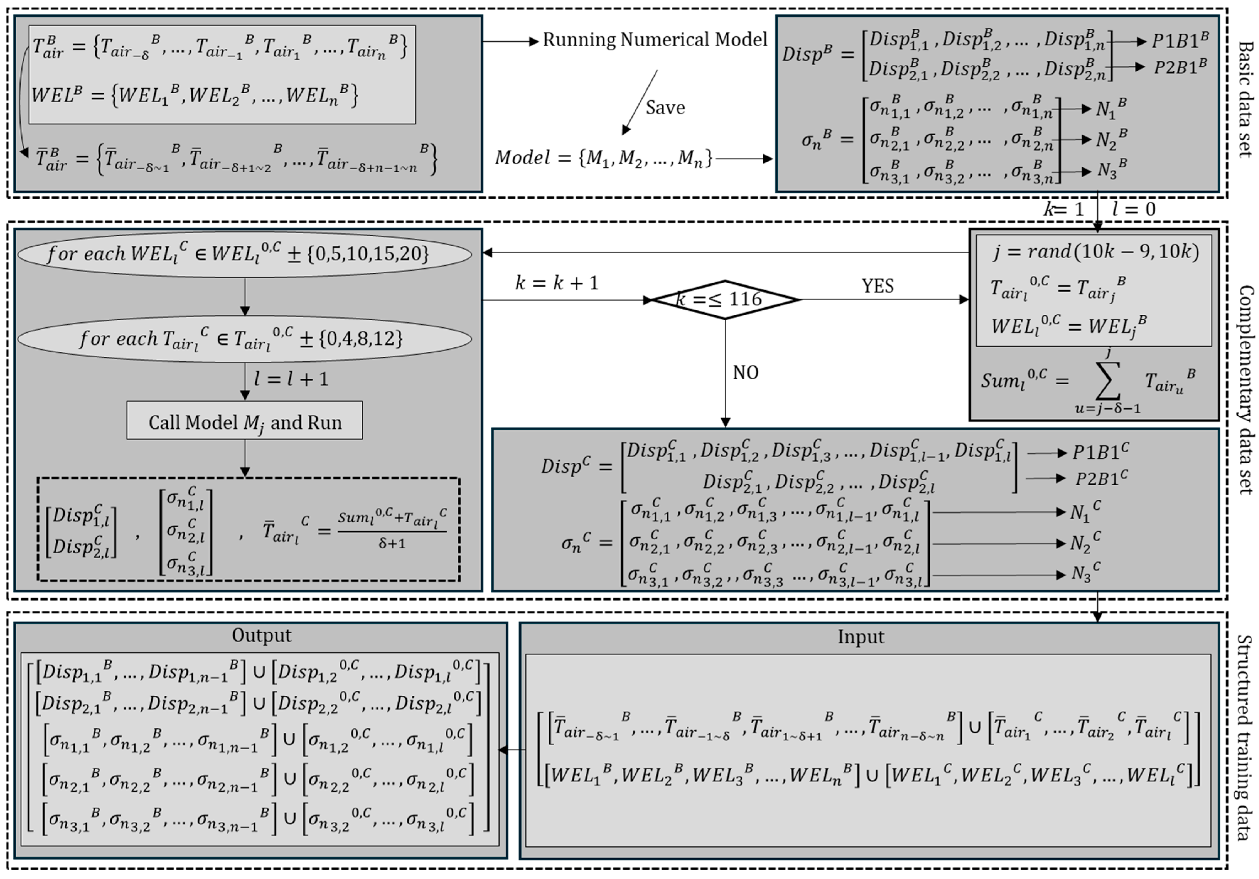
The training data consists of basic and complementary datasets, as illustrated in Figure 13. The basic training dataset is generated from the numerical simulation runs under the actual loading conditions, i.e., real water elevation and air temperature, experienced by the El Atazar dam from May 2020 to July 2023 (daily runs). This dataset comprises 1165 data points, with a runtime of 8640 s (2.4 h), executed on a personal laptop equipped with an Intel Core i7-12650H processor and 16 GB of RAM.
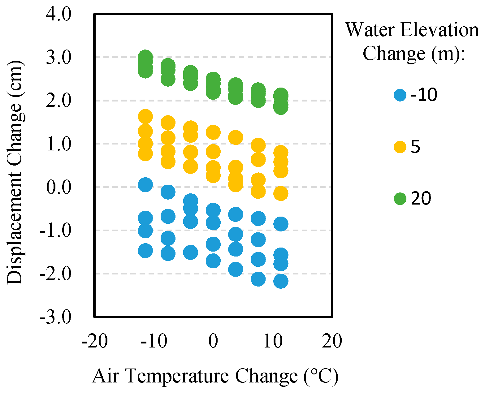
The complementary dataset is provided to cover the inexperienced loading scenarios. The primary numerical simulations indicate that the final stress-deformation state of arch dam-foundation systems is influenced not only by the final loading conditions, such as water elevation and air temperature, but also by the system’s initial state, as shown in Figure 14. This means that models with different initial stress-deformation states may respond differently to identical external loading due to the intrinsic nonlinearity of the arch dam system. In addition to this nonlinearity, the heat transfer between the dam’s interior and surface is significantly affected by the temperature differences between them, driven by the concrete’s thermal conductivity. Consequently, both the final ambient temperature and the concrete initial thermal condition determine the dam’s final thermal state. As a result of the factors discussed above, the long-term response of a high concrete dam is highly dependent on the loading path.
To account for a broader range of loading paths beyond the dam’s actual historical experience, several hypothetical loading scenarios are designed and analyzed using the numerical model. For this purpose, 116 days are selected randomly from the basic dataset (approximately one every ten days). This sampling density was chosen because the key input variables—water elevation and air temperature—exhibit relatively smooth, gradual temporal variation at El Atazar dam. Under these conditions, selecting one representative day per 10-day interval provides sufficient statistical diversity while avoiding redundant simulations. For dams where environmental or operational conditions fluctuate more abruptly, a denser sampling strategy (i.e., selecting additional days) would be required to ensure adequate statistical power and variability in the training dataset.
For each selected day, the analysis is extended by one additional day under a hypothetical loading path characterized by variations in water elevation and air temperature (Figure 15). These new loading conditions are carefully chosen to represent a wide range of possible unseen loading paths. In this article, the possible daily changes in water elevation and air temperature are limited to a maximum of 20 m and 12 °C, respectively:
37   m W E L d a y = i + 1 = W E L d a y = i ± 0,5 , 10,15,20 141.4   m
3.0   ° C T d a y = i + 1 = T d a y = i ± 0,4 , 8,12 37.0   ° C
where WEL and T represent the water elevation and air temperature, respectively. In total, 3655 additional data points are generated, requiring 8.1 h of running time. These new datasets also help reduce the extrapolation needed in LOESS prediction for unseen loading scenarios, thereby improving prediction accuracy.
After generating the dataset, the input and output variables are structured for the training model. In this study, the output variables are selected as the radial displacements of pendulums P1B1 and P2B1, along with the normal stress at crack surface points N1, N2, and N3, as defined in Figure 11. However, the methodology described here can be applied to predict other response variables as well. The input variables should be carefully selected to represent the most significant factors influencing the dam’s structural behavior. While some input variables directly impact response estimation, others may have a negligible influence and can be excluded from the model to enhance model efficiency.
Among the input variables, reservoir water elevation is widely recognized in the literature as a dominant factor in the dam’s response prediction due to its direct impact on hydrostatic loading [45,47,48,50,73,74].
As a thermal input variable representing the dam body’s temperature field, thermometer readings embedded within the concrete were available in this project and were used during the numerical model calibration stage. However, these measurements are not ideal for long-term predictive modeling because their records are often incomplete or discontinuous over time. Additionally, the objective of this study is to develop a methodology that is broadly applicable to various dam projects with differing instrumentation layouts and monitoring systems. In contrast, air temperature is typically measured continuously at dam sites, is readily available over long monitoring periods, and is less susceptible to sensor failure. Therefore, adopting air temperature as the thermal input variable enables the construction of a complete and consistent training dataset, reduces the dimensionality of the input matrix, and ensures that the proposed prediction framework remains robust and operational even in the absence of reliable internal temperature measurements in the future.
However, the influence of air temperature on the thermal field of the dam body is less straightforward than the influence of water elevation. This is because its effect depends not only on the temperature itself but also on the duration of exposure at the dam site. While the surface concrete temperature responds quickly to daily air temperature fluctuations, the internal thermal field reflects the past thermal conditions due to the concrete’s thermal inertia. A practical approach for addressing this time-dependent thermal effect and considering the cumulative thermal history of the dam is to use the mean air temperature over a specific number of preceding days, rather than the current daily temperature. The suitable number of days to be included in the mean air temperature calculation —denoted by δ in Figure 13—will be determined and discussed in Section 6.1. Consequently, in this study, the input variables used for model training are (1) the water elevation and (2) the mean air temperature over the last δ days.

5.2. The LOESS Model Setup

The LOESS model setup involves selecting the parameters p, q, and θ . In this study, p = 2 and q = 1 are selected for the orders of the mean and variance functions, respectively, as previous research has shown that these values offer a practical balance between accuracy and computational efficiency in dam engineering applications [70,75]. However, selecting θ is less straightforward, as it requires a trial-and-error effort to determine the number of training data that should be included in the kernel weighting calculation for each prediction. In this study, θ is identified individually for each input variable to minimize the prediction error. The details on θ selection will be presented in Section 6.2.

5.3. The Prediction Error Quantification

In this study, commonly used statistical error metrics, including mean absolute error (MAE), mean squared error (MSE), root mean squared error (RMSE), and the coefficient of determination ( R 2 ) are employed for standard error quantification:
M A E = 1 n i = 1 n y m o d e l ( i )   y p r e d i c t e d ( i )
M S E = 1 n i = 1 n ( y m o d e l ( i ) y p r e d i c t e d ( i ) ) 2
R M S E = 1 n i = 1 n ( y m o d e l ( i ) y p r e d i c t e d ( i ) ) 2
R 2 = 1 i = 1 n ( y m o d e l ( i ) y p r e d i c t e d ( i ) ) 2 i = 1 n ( y m o d e l ( i ) y ¯ m o d e l ) 2

6. Results and Discussion

6.1. Selection of δ

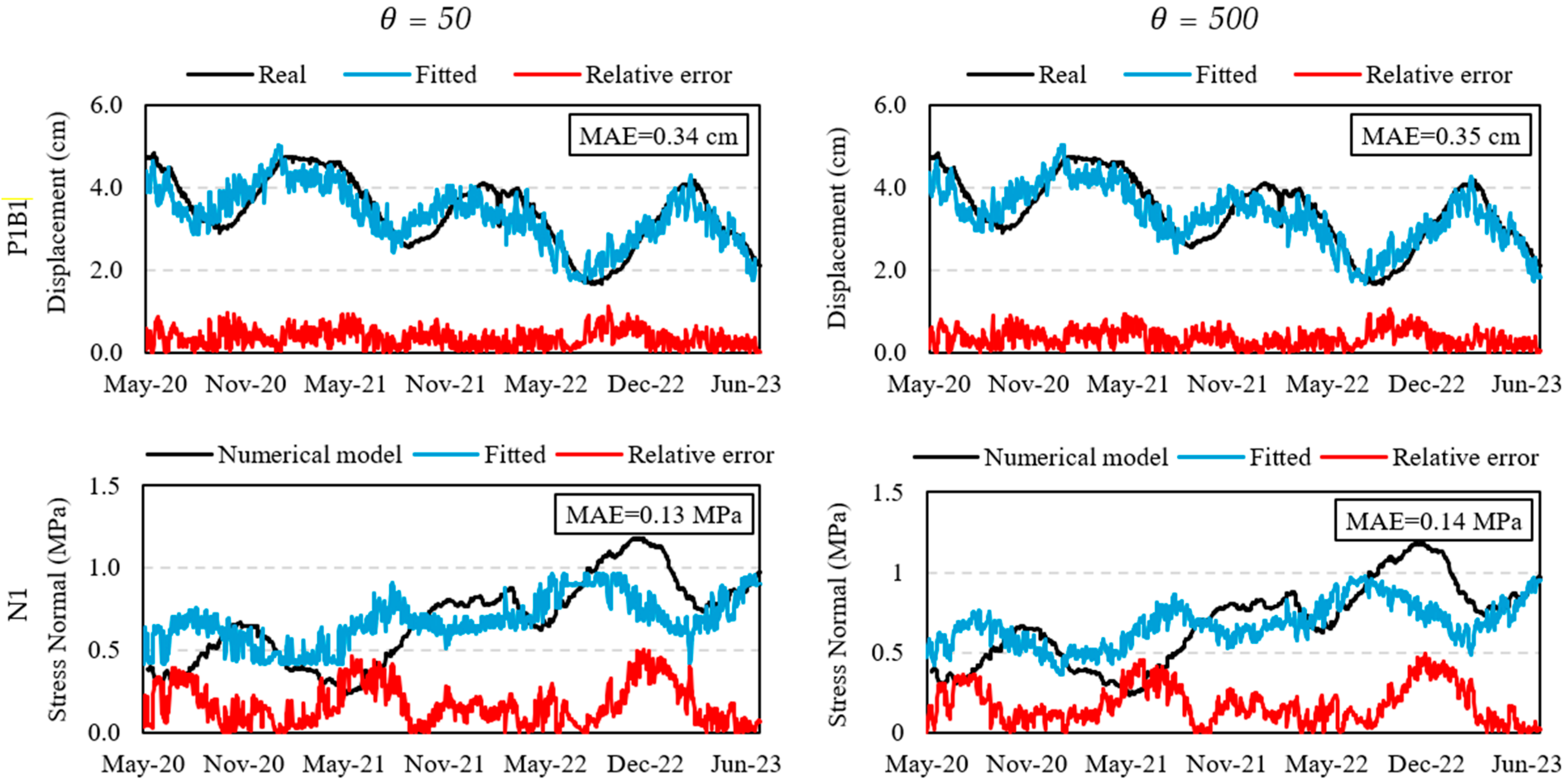
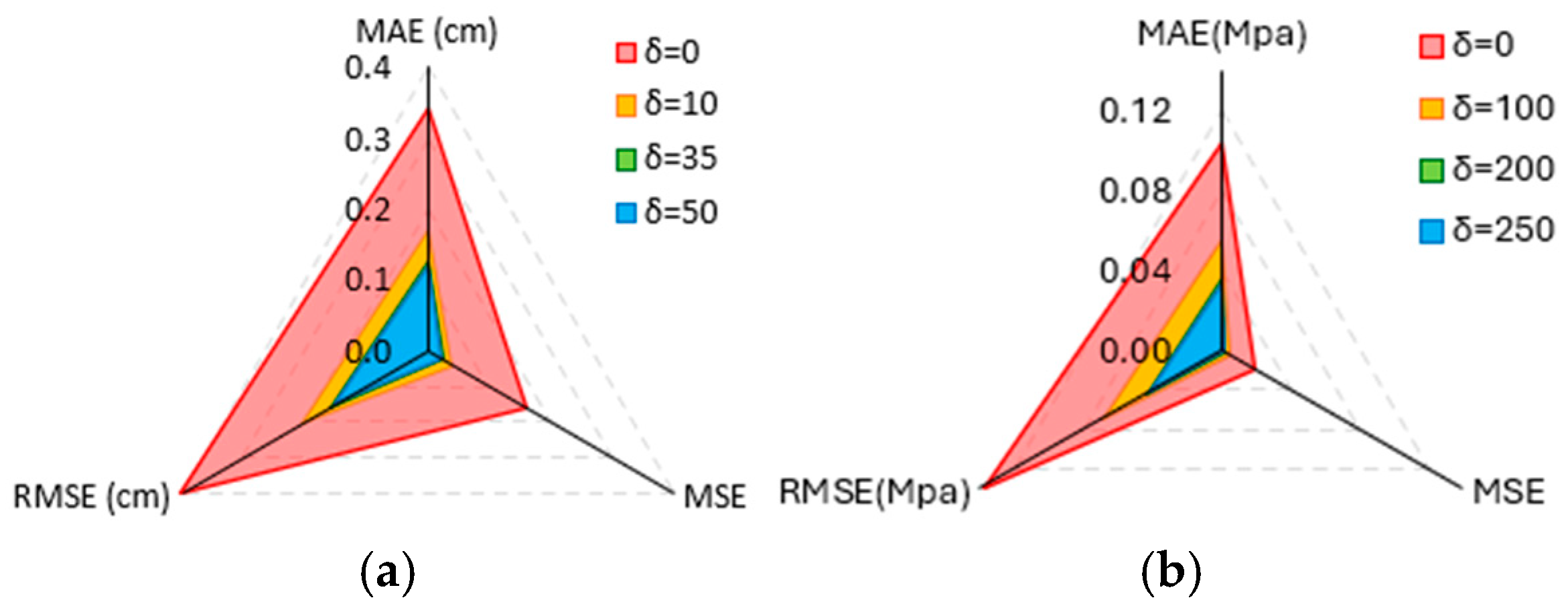
The initial step in response prediction involves filling the training dataset by determining the optimal δ value that accurately represents the concrete thermal field. Figure 16 (top left) illustrates the displacement fitting for P1B1 over the fitting dataset, assuming δ = 0, meaning that only the current air temperature is considered as the thermal loading variable in each prediction. In this case, it is assumed that the θ values for all the input variables are equal, set to 50. The resulting model yields an MAE of 0.34 cm. As shown in Figure 16, the fitted displacements exhibit excessive short-term fluctuations with a noticeable lag, closely following daily air temperature variations. Even when applying an over-smoothed model ( θ = 500 , Figure 16 (top right)), these high-frequency oscillations persist, indicating that short-term air temperature variations alone do not sufficiently capture the long-term thermal effects on the dam. These lags and over-fluctuations are even more pronounced when fitting the normal stress of N1 (Figure 16 (bottom left and right)). To address these issues, multiple fittings were performed for different values of δ, and the corresponding errors were calculated, as presented in Figure 17. The results indicate that using the mean air temperature over the past 35 days provides the best representation of the thermal field for fitting pendulum displacement, whereas a more extended averaging period of 200 days is optimal for fitting normal stress. The need for a higher δ in stress fitting compared to displacement fitting is due to the stress control points being located in the lower elevations of the dam body, where the thicker cantilever sections slow down heat transfer, thereby requiring a longer averaging period to accurately reflect the thermal effects.
It should be noted, however, that the values of 35 and 200 days represent the optimal choices for the specific points analyzed in this study, but other locations in the dam may require shorter or longer averaging periods to adequately capture their thermal behavior. These observations are consistent with multiple studies that show thermal loading produces a delayed response in concrete dams, as the dam’s internal temperature field evolves more slowly than the ambient air temperature due to heat diffusion through the massive concrete structure [76,77,78,79,80,81]. Empirical studies report lags of several weeks (e.g., ~30–40 days in some cases) [78], and modern monitoring approaches account for this using time-shifted correlations, lagged temperature terms, or heat-diffusion models [76,77,79,81]. It should also be noted that the magnitudes of lags between the extreme displacements and extreme air temperatures depend on the dam’s design and technical parameters. Consequently, these extremes and their representation periods vary for each dam.

6.2. Selection of θ

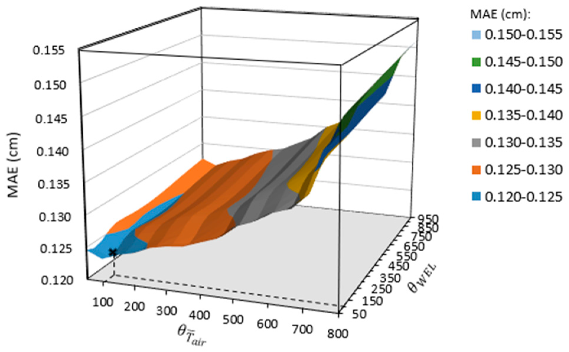
The θ values, which determine the bandwidth parameters, indicate the number of neighboring training data points included in each prediction. The proper θ value is determined separately for each input variable through an inverse trial-and-error process, aiming to minimize prediction error over the fitting dataset. An example of this process is shown in Figure 18, where the displacement of P1B1 is used for training. In this case, the optimal number of data points used for each displacement prediction is found to be 100 for both the water elevation and mean air temperature. For stress prediction, a larger θ value of 250 yields the best performance.

6.3. Final Fitting and Prediction Attempt

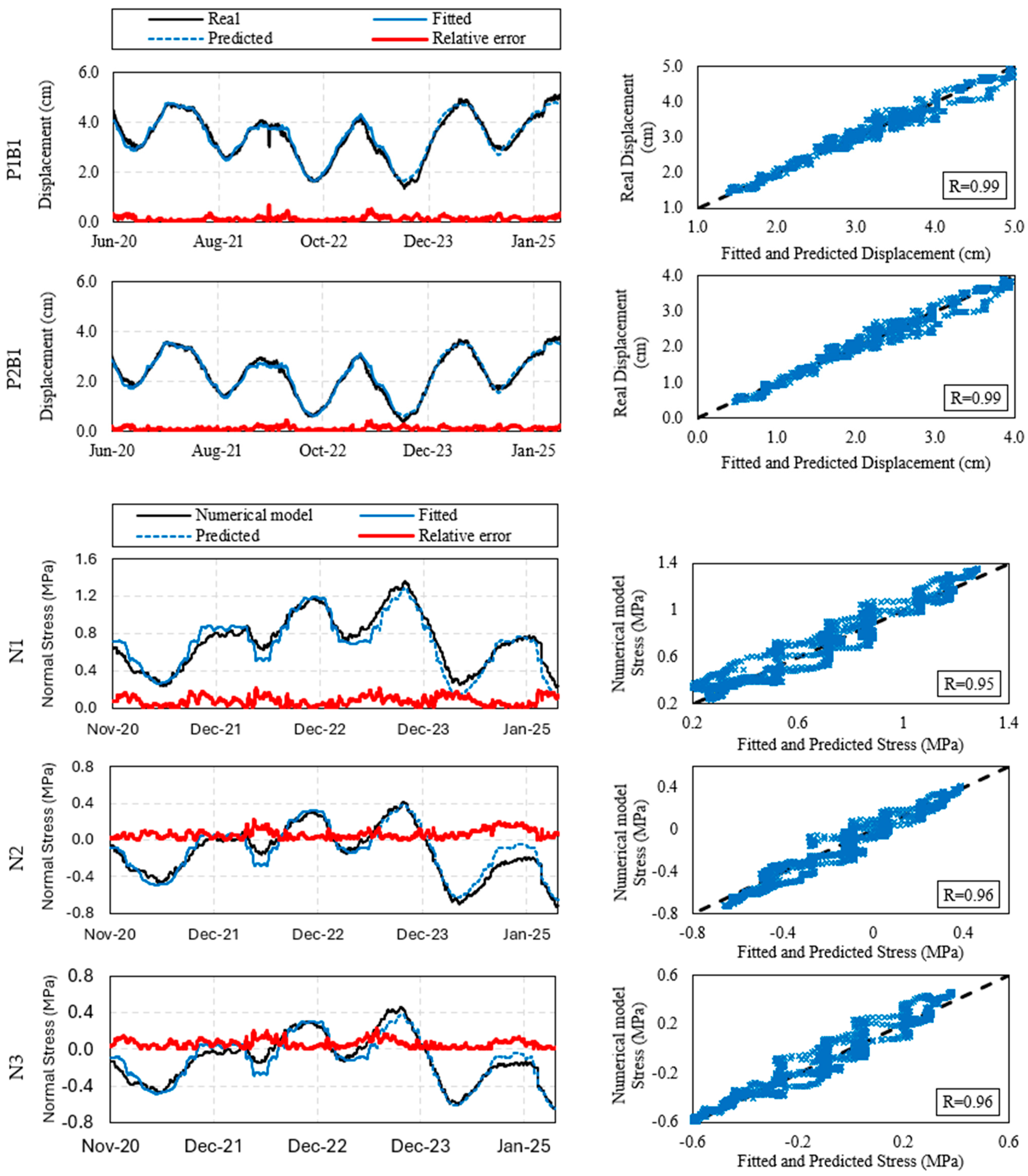
The final fitting and prediction results for both displacement and stress responses of the dam are illustrated in Figure 19. The left column presents the time-series comparison between the measured and predicted values for the selected monitoring points, including pendulum displacements (P1B1, P2B1) and normal stresses at crack-surface points (N1, N2, N3). The right column displays predicted versus measured scatter plots, which visually illustrate the agreement between model outputs and observations. It is worth mentioning that, for displacement prediction, the real values are based on the pendulum readings, whereas for stress prediction, the real values are those of the numerical model, as no site measurements are available. It should be noted that the reported stress represents variations driven by self-weight, thermal and hydraulic loading, as the absolute in situ stress state of a dam is inherently unknown due to long-term material evolution and multiple interacting historical effects.
As shown in Figure 19, the predicted values closely follow the observed data trends, demonstrating the strong capability of the developed model for predicting the response of the high concrete arch dam. A summary of the predicted errors is listed in Table 4. The MAE for displacement prediction is 0.12 and 0.09 cm for P1B1 and P2B1, respectively, indicating high accuracy in displacement prediction. The high correlation coefficients (R-values) of 0.99 for displacement predictions further highlight the model’s effectiveness in capturing the dam’s nonlinear behavior.
However, the stress prediction exhibits slightly larger deviations compared to displacement prediction, with correlation coefficients of 0.95, 0.96, and 0.96 for N1, N2, and N3, respectively. The corresponding MAE values are 0.077, 0.063, and 0.062 MPa for N1, N2, and N3, respectively. The lower precision in stress prediction can be attributed to the inherent complexity of stress distribution in a concrete arch dam. Stress is a second-order response variable in which slight variations in material properties or loading history can result in significant differences in stress distribution. Stress concentration can also occur in concrete due to several factors, such as local material heterogeneity, micro-crack propagation, and internal constraints within the dam body, while the displacements may remain unaffected. This hidden complexity makes stress prediction even more challenging in the context of concrete arch dam response prediction. Nevertheless, the presented model still shows reliable accuracy in stress predictions.
The proposed hybrid methodology can be further extended in future work to predict additional response variables, such as concrete temperature, joint opening, and dynamic responses. It can also be employed as a tool for structural health monitoring applications and maintenance planning by tracking the performance of concrete arch dams and other civil structures.

7. Conclusions

This study presents a novel hybrid approach that combines the Discrete Element Model (DEM) with the Locally Estimated Scatterplot Smoothing (LOESS) technique to predict the structural response of concrete arch dams. Unlike traditional parametric regression models that rely on a fixed regression function, the LOESS adapts dynamically to each input, allowing for a more accurate representation of highly nonlinear dam behavior without needing excessively complex machine learning techniques. The methodology was then applied to the El Atazar concrete arch dam to demonstrate its effectiveness in predicting both displacement and stress responses.
The study is divided into two steps. In the first step, a structured calibration strategy was proposed to enhance the accuracy of the numerical model. The calibration process consisted of two stages: first, the dam’s thermal field was adjusted by comparing simulated and observed temperature distributions. Once the temperature field was calibrated, the mechanical properties, including the elastic modulus of the concrete and foundation and the thermal expansion coefficient, were adjusted to align the model displacements with pendulum measurements for each day over a three-year period.
In the second step, the training dataset was generated entirely from the well-calibrated numerical model. This approach helps remove the influence of noisy or erroneous field data. However, an optional mechanism may allow for the integration of new monitoring data over time, enabling continuous model refinement. Another advantage of constructing the training dataset from numerical simulations is the ability to predict a wide range of structural responses, including deformation, stress, joint opening, and even dynamic responses. In this study, stress and displacement were selected to demonstrate the applicability of the methodology.
The training data consisted of basic and complementary datasets. The basic dataset was generated from numerical simulations under actual loading conditions, using recorded water elevation and air temperature data over a three-year period (with daily time steps). However, since results indicated that the dam’s final stress-deformation state is influenced not only by the final loading conditions but also by its initial state, a complementary dataset was introduced to account for previously unexperienced loading scenarios and different loading paths.
After generating the dataset, the input and output variables were structured for the training model. A key aspect of this study is identifying the optimal input variables for response prediction. A detailed analysis revealed that instead of using the current air temperature, employing the mean air temperature over the past 35 days improves displacement predictions, while a longer averaging period of 200 days is more suitable for stress prediction. The final predictive model was developed using the locally estimated scatterplot smoothing (LOESS) method, with polynomial orders of p = 2 and q = 1 for the mean and variance functions, respectively. The results showed a strong agreement between predicted and observed values.
It should be emphasized that the reliability of LOESS-based predictions depends directly on the quality and representativeness of the training data. Ensuring that the input data are accurate, unbiased, and reflective of actual operating conditions is therefore essential. In practice, engineers may implement continuous monitoring frameworks to evaluate the model’s performance over time and update it as new information becomes available.
The proposed hybrid methodology can be further extended in future work to predict additional response variables, such as concrete temperature, joint opening, and dynamic responses. It can also be employed as a powerful and adaptable tool for structural health monitoring applications and maintenance planning by tracking the performance of concrete arch dams and other civil structures. Compared to traditional methods, this technique requires less training data, making it ideal for dams with limited monitoring records—such as older dams or newly operated ones. Beyond arch dams, this approach can be applied to other nonlinear structures, making it a valuable asset for structural health monitoring and maintenance planning.

Author Contributions

Conceptualization, N.S., I.E.-B., and D.G.; data curation, I.E.-B. and D.G.; formal analysis, N.S.; funding acquisition, I.E.-B.; investigation, N.S.; methodology, N.S. and I.E.-B.; project administration, I.E.-B. and D.G.; resources, I.E.-B. and D.G.; software, N.S.; supervision, I.E.-B. and D.G.; validation, N.S., I.E.-B. and D.G.; visualization, N.S.; writing—original draft, N.S.; writing—review and editing, N.S. All authors have read and agreed to the published version of the manuscript.

Funding

This research received no external funding.

Data Availability Statement

The original contributions presented in this study are included in this article, further inquiries can be directed to the corresponding author.

Conflicts of Interest

Author David Galán was employed by the company Canal de Isabel II. Canal de Isabel II provided access to the data and numerical models used in this study. No financial support related to the aim and results of this research was provided by Canal de Isabel II.

References

  1. Chelidze, T.; Matcharashvili, T.; Abashidze, V.; Kalabegishvili, M.; Zhukova, N. Real time monitoring for analysis of dam stability: Potential of nonlinear elasticity and nonlinear dynamics approaches. Front. Struct. Civ. Eng. 2013, 7, 188–205. [Google Scholar] [CrossRef]
  2. Clarkson, L.; Williams, D.; Seppälä, J. Real-time monitoring of tailings dams. Georisk Assess. Manag. Risk Eng. Syst. Geohazards 2021, 15, 113–127. [Google Scholar] [CrossRef]
  3. Ren, Q.; Li, M.; Kong, T.; Ma, J. Multi-sensor real-time monitoring of dam behavior using self-adaptive online sequential learning. Autom. Constr. 2022, 140, 104365. [Google Scholar] [CrossRef]
  4. Chen, N.; Li, B.; Wang, Y.; Ying, X.; Wang, L.; Zhang, C.; Guo, Y.; Li, M.; An, W. Motion and Appearance Decoupling Representation for Event Cameras. IEEE Trans. Image Process. 2025, 34, 5964–5977. [Google Scholar] [CrossRef]
  5. Adamo, N.; Al-Ansari, N.; Ali, S.H.; Laue, J.; Knutsson, S. Dams safety: Review of satellite remote sensing applications to dams and reservoirs. J. Earth Sci. Geotech. Eng. 2021, 11, 347–438. [Google Scholar] [CrossRef]
  6. Chang, Y.; Chang, L.; Chang, F. Intelligent control for modeling of real-time reservoir operation, part II: Artificial neural network with operating rule curves. Hydrol. Process. Int. J. 2005, 19, 1431–1444. [Google Scholar] [CrossRef]
  7. Gomes, M.G.; da Silva, V.H.C.; Pinto, L.F.R.; Centoamore, P.; Digiesi, S.; Facchini, F.; Neto, G.C.d.O. Economic, environmental and social gains of the implementation of artificial intelligence at dam operations toward Industry 4.0 principles. Sustainability 2020, 12, 3604. [Google Scholar] [CrossRef]
  8. Yang, T.; Zhang, L.; Kim, T.; Hong, Y.; Zhang, D.; Peng, Q. A large-scale comparison of Artificial Intelligence and Data Mining (AI&DM) techniques in simulating reservoir releases over the Upper Colorado Region. J. Hydrol. 2021, 602, 126723. [Google Scholar]
  9. Serradilla, O.; Zugasti, E.; Rodriguez, J.; Zurutuza, U. Deep learning models for predictive maintenance: A survey, comparison, challenges and prospects. Appl. Intell. 2022, 52, 10934–10964. [Google Scholar] [CrossRef]
  10. Kumar, K.; Saini, R.P. A review on operation and maintenance of hydropower plants. Sustain. Energy Technol. Assess. 2022, 49, 101704. [Google Scholar] [CrossRef]
  11. Haenlein, M.; Kaplan, A. A brief history of artificial intelligence: On the past, present, and future of artificial intelligence. Calif. Manag. Rev. 2019, 61, 5–14. [Google Scholar] [CrossRef]
  12. Jordan, M.I.; Mitchell, T.M. Machine learning: Trends, perspectives, and prospects. Science 2015, 349, 255–260. [Google Scholar] [CrossRef]
  13. Hopgood, A.A. Intelligent Systems for Engineers and Scientists: A Practical Guide to Artificial Intelligence; CRC Press: Boca Raton, FL, USA, 2021. [Google Scholar]
  14. Abdollahi, A.; Amini, A.; Hariri-Ardebili, M.A. An uncertainty-aware dynamic shape optimization framework: Gravity dam design. Reliab. Eng. Syst. Saf. 2022, 222, 108402. [Google Scholar] [CrossRef]
  15. CASE Arch Dam Task Group. User’s Guide: Arch Dam Stress Analysis System (ADSAS); US Army: Washington, DC, USA, 1997. [Google Scholar]
  16. Flah, M.; Nunez, I.; Ben Chaabene, W.; Nehdi, M.L. Machine learning algorithms in civil structural health monitoring: A systematic review. Arch. Comput. Methods Eng. 2021, 28, 2621–2643. [Google Scholar] [CrossRef]
  17. Hariri-Ardebili, M.A.; Pourkamali-Anaraki, F. An automated machine learning engine with inverse analysis for seismic design of dams. Water 2022, 14, 3898. [Google Scholar] [CrossRef]
  18. Hamidian, D.; Seyedpoor, S.M. Shape optimal design of arch dams using an adaptive neuro-fuzzy inference system and improved particle swarm optimization. Appl. Math. Model. 2010, 34, 1574–1585. [Google Scholar] [CrossRef]
  19. Jehanzaib, M.; Shah, S.A.; Son, H.J.; Jang, S.-H.; Kim, T.-W. Predicting hydrological drought alert levels using supervised machine-learning classifiers. KSCE J. Civ. Eng. 2022, 26, 3019–3030. [Google Scholar] [CrossRef]
  20. Cheng, M.-Y.; Cao, M.-T.; Huang, I.-F. Hybrid artificial intelligence-based inference models for accurately predicting dam body displacements: A case study of the Fei Tsui dam. Struct. Health Monit. 2022, 21, 1738–1756. [Google Scholar] [CrossRef]
  21. Jing, Z.; Gao, X. Monitoring and early warning of a metal mine tailings pond based on a deep learning bidirectional recurrent long and short memory network. PLoS ONE 2022, 17, e0273073. [Google Scholar] [CrossRef]
  22. Himeur, Y.; Ghanem, K.; Alsalemi, A.; Bensaali, F.; Amira, A. Artificial intelligence based anomaly detection of energy consumption in buildings: A review, current trends and new perspectives. Appl. Energy 2021, 287, 116601. [Google Scholar] [CrossRef]
  23. Su, H.; Wen, Z.; Wu, Z. Study on an intelligent inference engine in early-warning system of dam health. Water Resour. Manag. 2011, 25, 1545–1563. [Google Scholar] [CrossRef]
  24. Hariri-Ardebili, M.A.; Sudret, B. Polynomial chaos expansion for uncertainty quantification of dam engineering problems. Eng. Struct. 2020, 203, 109631. [Google Scholar] [CrossRef]
  25. Kalinina, A.; Spada, M.; Vetsch, D.F.; Marelli, S.; Whealton, C.; Burgherr, P.; Sudret, B. Metamodeling for uncertainty quantification of a flood wave model for concrete dam breaks. Energies 2020, 13, 3685. [Google Scholar] [CrossRef]
  26. Lin, C.; Li, T.; Chen, S.; Yuan, L.; van Gelder, P.; Yorke-Smith, N. Long-term viscoelastic deformation monitoring of a concrete dam: A multi-output surrogate model approach for parameter identification. Eng. Struct. 2022, 266, 114553. [Google Scholar] [CrossRef]
  27. Tong, F.; Yang, J.; Ma, C.; Cheng, L.; Li, G. The prediction of concrete dam displacement using Copula-PSO-ANFIS hybrid model. Arab. J. Sci. Eng. 2022, 47, 4335–4350. [Google Scholar] [CrossRef]
  28. Pacheco, F.; Hermosilla, G.; Piña, O.; Villavicencio, G.; Allende-Cid, H.; Palma, J.; Valenzuela, P.; García, J.; Carpanetti, A.; Minatogawa, V. Generation of synthetic data for the analysis of the physical stability of tailing dams through artificial intelligence. Mathematics 2022, 10, 4396. [Google Scholar] [CrossRef]
  29. Qi, C.; Tang, X. Slope stability prediction using integrated metaheuristic and machine learning approaches: A comparative study. Comput. Ind. Eng. 2018, 118, 112–122. [Google Scholar] [CrossRef]
  30. Lin, C.; Chen, S.; Hariri-Ardebili, M.A.; Li, T. An explainable probabilistic model for health monitoring of concrete dam via optimized sparse bayesian learning and sensitivity analysis. Struct. Control Health Monit. 2023, 2023, 2979822. [Google Scholar] [CrossRef]
  31. Zhang, K.; Gu, C.; Zhu, Y.; Li, Y.; Shu, X. A mathematical-mechanical hybrid driven approach for determining the deformation monitoring indexes of concrete dam. Eng. Struct. 2023, 277, 115353. [Google Scholar] [CrossRef]
  32. Wei, B.; Luo, S.; Yuan, D. Optimized combined forecasting model for hybrid signals in the displacement monitoring data of concrete dams. In Structures; Elsevier: Amsterdam, The Netherlands, 2023; pp. 1989–2002. [Google Scholar]
  33. Tao, L.; Zheng, D.; Wu, X.; Chen, X.; Liu, Y.; Chen, Z.; Jiang, H. Stress estimation of concrete dams in service based on deformation data using SIE–APSO–CNN–LSTM. Water 2022, 15, 59. [Google Scholar] [CrossRef]
  34. Mata, J.; Miranda, F.; Antunes, A.; Romão, X.; Pedro Santos, J. Characterization of relative movements between blocks observed in a concrete dam and definition of thresholds for novelty identification based on machine learning models. Water 2023, 15, 297. [Google Scholar] [CrossRef]
  35. He, M.; Li, H.; Xu, J.; Wang, H.; Xu, W.; Chen, S. Estimation of unloading relaxation depth of Baihetan Arch Dam foundation using long-short term memory network. Water Sci. Eng. 2021, 14, 149–158. [Google Scholar] [CrossRef]
  36. Wang, S.; Sui, X.; Liu, Y.; Gu, H.; Xu, B.; Xia, Q. Prediction and interpretation of the deformation behaviour of high arch dams based on a measured temperature field. J. Civ. Struct. Health Monit. 2023, 13, 661–675. [Google Scholar] [CrossRef]
  37. Hariri-Ardebili, M.A.; Mahdavi, G.; Nuss, L.K.; Lall, U. The role of artificial intelligence and digital technologies in dam engineering: Narrative review and outlook. Eng. Appl. Artif. Intell. 2023, 126, 106813. [Google Scholar] [CrossRef]
  38. Zhang, Y.; Zhang, W.; Li, Y.; Wen, L.; Sun, X. A multi-output prediction model for the high arch dam displacement utilizing the VMD-DTW partitioning technique and long-term temperature. Expert Syst. Appl. 2025, 267, 126135. [Google Scholar] [CrossRef]
  39. Li, S.; Zhang, B.; Yang, M.; Li, S.; Liu, Z. A New Prediction Model of Dam Deformation and Successful Application. Buildings 2025, 15, 818. [Google Scholar] [CrossRef]
  40. Liu, M.; Feng, Y.; Yang, S.; Su, H. Dam deformation prediction considering the seasonal fluctuations using ensemble learning algorithm. Buildings 2024, 14, 2163. [Google Scholar] [CrossRef]
  41. Li, M.; Ren, Q.; Li, M.; Fang, X.; Xiao, L.; Li, H. A separate modeling approach to noisy displacement prediction of concrete dams via improved deep learning with frequency division. Adv. Eng. Inform. 2024, 60, 102367. [Google Scholar] [CrossRef]
  42. Shao, C.; Xu, Y.; Chen, H.; Zheng, S.; Qin, X. Ordinary Kriging interpolation method combined with FEM for arch dam deformation field estimation. Mathematics 2023, 11, 1106. [Google Scholar] [CrossRef]
  43. Liu, B.; Wei, B.; Li, H.; Mao, Y. Multipoint hybrid model for RCC arch dam displacement health monitoring considering construction interface and its seepage. Appl. Math. Model. 2022, 110, 674–697. [Google Scholar] [CrossRef]
  44. Xiong, F.; Wei, B.; Xu, F.; Zhou, L. Deterministic combination prediction model of concrete arch dam displacement based on residual correction. In Structures; Elsevier: Amsterdam, The Netherlands, 2022; pp. 1011–1024. [Google Scholar]
  45. Lin, C.; Weng, K.; Lin, Y.; Zhang, T.; He, Q.; Su, Y. Time series prediction of dam deformation using a hybrid STL–CNN–GRU model based on sparrow search algorithm optimization. Appl. Sci. 2022, 12, 11951. [Google Scholar] [CrossRef]
  46. He, Q.; Gu, C.; Valente, S.; Zhao, E.; Liu, X.; Yuan, D. Multi-arch dam safety evaluation based on statistical analysis and numerical simulation. Sci. Rep. 2022, 12, 8913. [Google Scholar] [CrossRef] [PubMed]
  47. Wei, B.; Liu, B.; Yuan, D.; Mao, Y.; Yao, S. Spatiotemporal hybrid model for concrete arch dam deformation monitoring considering chaotic effect of residual series. Eng. Struct. 2021, 228, 111488. [Google Scholar] [CrossRef]
  48. Wang, S.; Xu, C.; Gu, C.; Su, H.; Wu, B. Hydraulic-seasonal-time-based state space model for displacement monitoring of high concrete dams. Trans. Inst. Meas. Control. 2021, 43, 3347–3359. [Google Scholar] [CrossRef]
  49. Salazar, F.; Conde, A.; Vicente, D.J. Identification of dam behavior by means of machine learning classification models. In Numerical Analysis of Dams: Proceedings of the 15th ICOLD International Benchmark Workshop 15; Springer: Berlin/Heidelberg, Germany, 2021; pp. 851–862. [Google Scholar]
  50. Shao, C.; Gu, C.; Meng, Z.; Hu, Y. Integrating the finite element method with a data-driven approach for dam displacement prediction. Adv. Civ. Eng. 2020, 2020, 4961963. [Google Scholar] [CrossRef]
  51. Wang, S.; Xu, C.; Gu, C.; Su, H.; Hu, K.; Xia, Q. Displacement monitoring model of concrete dams using the shape feature clustering-based temperature principal component factor. Struct. Control Health Monit. 2020, 27, e2603. [Google Scholar] [CrossRef]
  52. Yin, W.; Zhao, E.; Gu, C.; Huang, H.; Yang, Y. A nonlinear method for component separation of dam effect quantities using kernel partial least squares and pseudosamples. Adv. Civ. Eng. 2019, 2019, 1958173. [Google Scholar] [CrossRef]
  53. Wang, S.; Xu, Y.; Gu, C.; Bao, T.; Xia, Q.; Hu, K. Hysteretic effect considered monitoring model for interpreting abnormal deformation behavior of arch dams: A case study. Struct. Control Health Monit. 2019, 26, e2417. [Google Scholar] [CrossRef]
  54. Liu, C.; Gu, C.; Chen, B. Zoned elasticity modulus inversion analysis method of a high arch dam based on unconstrained Lagrange support vector regression (support vector regression arch dam). Eng. Comput. 2017, 33, 443–456. [Google Scholar] [CrossRef]
  55. Myers, R.H. Classical and Modern Regression with Applications; Duxbury Press: Belmont, CA, USA, 1990. [Google Scholar]
  56. John Lu, Z.Q. The elements of statistical learning: Data mining, inference, and prediction. J. R. Stat. Soc. Ser. A Stat. Soc. 2010, 173, 693–694. [Google Scholar]
  57. Altman, N.S. An introduction to kernel and nearest-neighbor nonparametric regression. Am. Stat. 1992, 46, 175–185. [Google Scholar] [CrossRef]
  58. Storlie, C.B.; Helton, J.C. Multiple predictor smoothing methods for sensitivity analysis: Description of techniques. Reliab. Eng. Syst. Saf. 2008, 93, 28–54. [Google Scholar] [CrossRef]
  59. Da Veiga, S.; Wahl, F.; Gamboa, F. Local polynomial estimation for sensitivity analysis on models with correlated inputs. Technometrics 2009, 51, 452–463. [Google Scholar] [CrossRef]
  60. Fan, J.; Gijbels, I. Variable bandwidth and local linear regression smoothers. Ann. Stat. 1992, 20, 2008–2036. [Google Scholar] [CrossRef]
  61. Fan, J.; Gijbels, I. Adaptive order polynomial fitting: Bandwidth robustification and bias reduction. J. Comput. Graph. Stat. 1995, 4, 213–227. [Google Scholar] [CrossRef]
  62. Wang, H.; Xu, D. Parameter selection method for support vector regression based on adaptive fusion of the mixed kernel function. J. Control. Sci. Eng. 2017, 2017, 3614790. [Google Scholar] [CrossRef]
  63. Canal de Isabel II. Documento XYZT de la Presa de El Atazar; Internal Technical Report; Canal de Isabel II: Madrid, Spain, 2002. [Google Scholar]
  64. Itasca Consulting Group, Inc. FLAC3D: Fast Lagrangian Analysis of Continua in 3 Dimensions; Itasca Consulting Group, Inc.: Minneapolis, MN, USA, 2020. [Google Scholar]
  65. ICOLD. Guidelines for Use of Numerical Models in Dam Engineering; International Commission on Large Dams: Paris, France, 2013. [Google Scholar]
  66. Soltani, N.; Escuder Bueno, I. Effect of Contraction and Construction Joint Quality on the Static Performance of Concrete Arch Dams. Infrastructures 2024, 9, 231. [Google Scholar] [CrossRef]
  67. Soltani, N.; Escuder-Bueno, I.; Klun, M. System Reliability Analysis of Concrete Arch Dams Considering Foundation Rock Wedges Movement: A Discussion on the Limit Equilibrium Method. Infrastructures 2024, 9, 176. [Google Scholar] [CrossRef]
  68. Bofang, Z. Thermal Stresses and Temperature Control of Mass Concrete; Butterworth-Heinemann: Oxford, UK, 2013. [Google Scholar]
  69. Léger, P.; Venturelli, J.; Bhattacharjee, S.S. Seasonal temperature and stress distributions in concrete gravity dams. Part 1: Modelling. Can. J. Civ. Eng. 1993, 20, 999–1017. [Google Scholar] [CrossRef]
  70. Ahmadi, M.T.; Soltani, N. Mixing Regression-Global Sensitivity analysis of concrete arch dam system safety considering foundation and abutment uncertainties. Comput. Geotech. 2021, 139, 104368. [Google Scholar] [CrossRef]
  71. Khaneghahi, M.H.; Alembagheri, M.; Soltani, N. Reliability and variance-based sensitivity analysis of arch dams during construction and reservoir impoundment. Front. Struct. Civ. Eng. 2019, 13, 526–541. [Google Scholar] [CrossRef]
  72. Soltani, N.; Alembagheri, M.; Khaneghahi, M.H. Risk-based probabilistic thermal-stress analysis of concrete arch dams. Front. Struct. Civ. Eng. 2019, 13, 1007–1019. [Google Scholar] [CrossRef]
  73. Wei, B.; Chen, L.; Li, H.; Yuan, D.; Wang, G. Optimized prediction model for concrete dam displacement based on signal residual amendment. Appl. Math. Model. 2020, 78, 20–36. [Google Scholar] [CrossRef]
  74. Yuan, D.; Gu, C.; Wei, B.; Qin, X.; Xu, W. A high-performance displacement prediction model of concrete dams integrating signal processing and multiple machine learning techniques. Appl. Math. Model. 2022, 112, 436–451. [Google Scholar] [CrossRef]
  75. Ruppert, D.; Wand, M.P.; Holst, U.; HöSJER, O. Local polynomial variance-function estimation. Technometrics 1997, 39, 262–273. [Google Scholar] [CrossRef]
  76. Ju, H.; Zhai, W.; Deng, Y.; Chen, M.; Li, A. Temperature time-lag effect elimination method of structural deformation monitoring data for cable-stayed bridges. Case Stud. Therm. Eng. 2023, 42, 102696. [Google Scholar] [CrossRef]
  77. Yigit, C.O.; Alcay, S.; Ceylan, A. Displacement response of a concrete arch dam to seasonal temperature fluctuations and reservoir level rise during the first filling period: Evidence from geodetic data. Geomat. Nat. Hazards Risk 2016, 7, 1489–1505. [Google Scholar] [CrossRef]
  78. Tretyak, K.; Palianytsia, B. Research of seasonal deformations of the Dnipro HPP dam according to GNSS measurements. Geodynamics 2021, 1, 5–16. [Google Scholar] [CrossRef]
  79. Cao, X.; Sheng, J.; Jiang, C.; Yuan, D.; Zhang, H. Concrete dam deformation prediction model considering the time delay of monitoring variables. Sci. Rep. 2025, 15, 8458. [Google Scholar] [CrossRef] [PubMed]
  80. Cao, W.; Wen, Z.; Feng, Y.; Zhang, S.; Su, H. A multi-point joint prediction model for high-arch dam deformation considering spatial and temporal correlation. Water 2024, 16, 1388. [Google Scholar] [CrossRef]
  81. Santillán, D.; Salete, E.; Toledo, M.Á. A new 1D analytical model for computing the thermal field of concrete dams due to the environmental actions. Appl. Therm. Eng. 2015, 85, 160–171. [Google Scholar] [CrossRef]
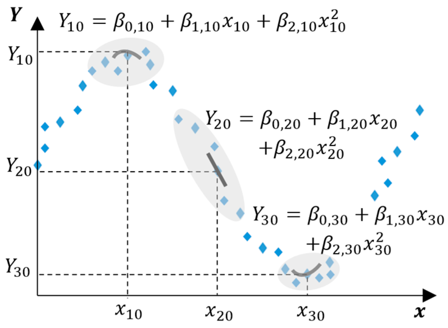
Figure 1. An example of a local prediction model for three different values of the input variable (training input) x using a quadratic local function.
Infrastructures 11 00009 g001
Figure 2. Effect of smoothing parameters on the prediction result.
Infrastructures 11 00009 g002
Figure 3. Representation of the 3-dimensional matrix of regression coefficients. Here, β p , n d denotes the p-th regression coefficient corresponding to sample point n and input variable d.
Infrastructures 11 00009 g003
Figure 4. El Atazar dam: (a) downstream view and (b) layout plan.
Infrastructures 11 00009 g004
Figure 5. The discrete element model of the El Atazar dam: (a) the 3-dimensional view of the dam and foundation, (b) the dam body mesh, (c) the vertical and peripheral joints, and (d) the downstream view of the injected crack surface.
Infrastructures 11 00009 g005
Figure 6. The yield surface used for the dam body concrete. Here, σ 1 , σ 3 , f t , f c , c , and φ are the minimum and maximum principal stress, uniaxial tensile and compressive strength, cohesion, and friction angle, respectively.
Infrastructures 11 00009 g006
Figure 7. The loading sequential process. Variables marked with (*) represent calibration parameters, while the rest are considered deterministic.
Infrastructures 11 00009 g007
Figure 8. The reservoir water elevation and the mean daily air temperature variation.
Infrastructures 11 00009 g008
Figure 9. Comparison of nodal temperatures on the upstream surface of the central cantilever between the model and thermometer readings for two specific days.
Infrastructures 11 00009 g009
Figure 10. Comparison of the concrete temperature in the central block between the numerical model and thermometer readings.
Infrastructures 11 00009 g010
Figure 11. Upstream view of the dam body showing the pendulum points used for displacement calibration.
Infrastructures 11 00009 g011
Figure 12. Comparison of the radial displacement in the numerical model with the pendulum’s readings.
Infrastructures 11 00009 g012
Figure 13. The flowchart of the training data preparation process. B, C, and n denote the basic dataset, complementary dataset, and day index, respectively. T a i r n and W E L n represent the air temperature and water elevation on day n, respectively. T ¯ a i r i ~ j is the mean air temperature from day i to j.  M n denotes the saved numerical model for day n. Disp and σ n   represent the displacement and normal stress, respectively. All remaining parameters were defined previously.
Infrastructures 11 00009 g013
Figure 14. The effect of the initial condition on the dam displacement. The models with different initial conditions respond differently to identical external loading.
Infrastructures 11 00009 g014
Figure 15. An example of the complementary loading paths for day j.
Infrastructures 11 00009 g015
Figure 16. The comparison between the real and fitted values assuming δ = 0.
Infrastructures 11 00009 g016
Figure 17. The error values for different values of δ in the fitting of (a) the displacement of P1B1 and (b) the normal stress of N1.
Infrastructures 11 00009 g017
Figure 18. The relationship between the calculated error in P1B1 displacement fitting and the θ values.
Infrastructures 11 00009 g018
Figure 19. The final fitting and prediction results.
Infrastructures 11 00009 g019
Table 1. A selected list of the latest studies on the displacement prediction of concrete arch dams.
YearAlgorithmReference
2025Variational Model Decomposition and Dynamic Time Warping[38]
2025Particle Swarm, EEMD-Wavelet Noise Reduction Algorithm[39]
2024XGBoost and TPE Optimization Algorithm[40]
2024Frequency-division decomposition and deep neural networks[41]
2023FEM *, Multi-Layer Perceptron[31]
2023Kriging Interpolation Method[42]
2022FEM *, Multipoint Hybrid, Multiple Linear Regression[43]
2022FEM *, Long Short-Term Memory Network, Auto-Regressive Integrated Moving Average[44]
2022Numerical model, Convolutional Neural Network, Long Short-Term Memory, Gated Recurrent Unit, Sparrow Search Optimization[45]
2022FEM *, Multiple Linear Stepwise Regression[46]
2021FEM *, Support Vector Machine, Particle Swarm Optimization[47]
2021FEM *, Hydraulic-Seasonal-Time-Based State Space Model, Kalman Filter Algorithm Optimization[48]
2021FEM *, Machine Learning Classification Model[49]
2020FEM *, Random Coefficient Model[50]
2020FEM *, Feature-Based Spatial Clustering[51]
2019FEM *, Kernel Partial Least Squares[52]
2019FEM *, Hydraulic-Hysteretic-Seasonal-Time Model[53]
2017FEM *, Unconstrained Lagrange Support Vector Regression, Culture Genetic Algorithm[54]
2011FEM *, Wavelet Networks, Rough Sets Theory[23]
* Finite Element Model.
Table 2. The calibrated thermal variables.
VariableCalibrated Value
Conductivity   ( W / ( m 2 °C))3.5
Specific Heat (J/(kg °C))967.0
Convection   Coefficient   ( W / ( m 2 °C))20.90
H D e e p (m)88.0
T D e e p (°C)6.5
Delay Value (days)7.0
Solar Radiation Effect (°C)+3.0
Table 3. The mechanical parameters used in the numerical model.
VariableConcreteFoundationVertical JointsPeripheral Joint
LeftRight
E (GPa)30.0 *5.0 *15.0 *--
ν0.270.330.33--
ρ (kg/m3)250028502850--
f c (MPa)32.0----
f t (MPa)3.0---1.5
Shear Stiffness (GPa/m)---4.07.0
Normal Stiffness (GPa/m)---40.040.0
φ (°)56.0--40.056.0
C (MPa)4.9--0.03.0
Expansion Coef. (1/°C) 6.5   × 10 6 *----
* Calibrated Values.
Table 4. A summary of the errors in the final prediction.
Prediction VariableMAE (cm)MSERMSE (cm)R
FittedPredictedFittedPredictedFittedPredictedFittedPredicted
P1B10.1200.1250.0250.0230.1590.1510.980.99
P2B10.0940.0950.0150.0130.1240.1150.990.99
Prediction variableMAE (MPa)MSERMSE (MPa)R
FittedPredictedFittedPredictedFittedPredictedFittedPredicted
N10.0760.0780.0080.0090.0880.0960.940.95
N20.0560.0730.0040.0080.0660.0920.960.97
N30.0690.0530.0060.0050.0800.0700.970.96
Disclaimer/Publisher’s Note: The statements, opinions and data contained in all publications are solely those of the individual author(s) and contributor(s) and not of MDPI and/or the editor(s). MDPI and/or the editor(s) disclaim responsibility for any injury to people or property resulting from any ideas, methods, instructions or products referred to in the content.