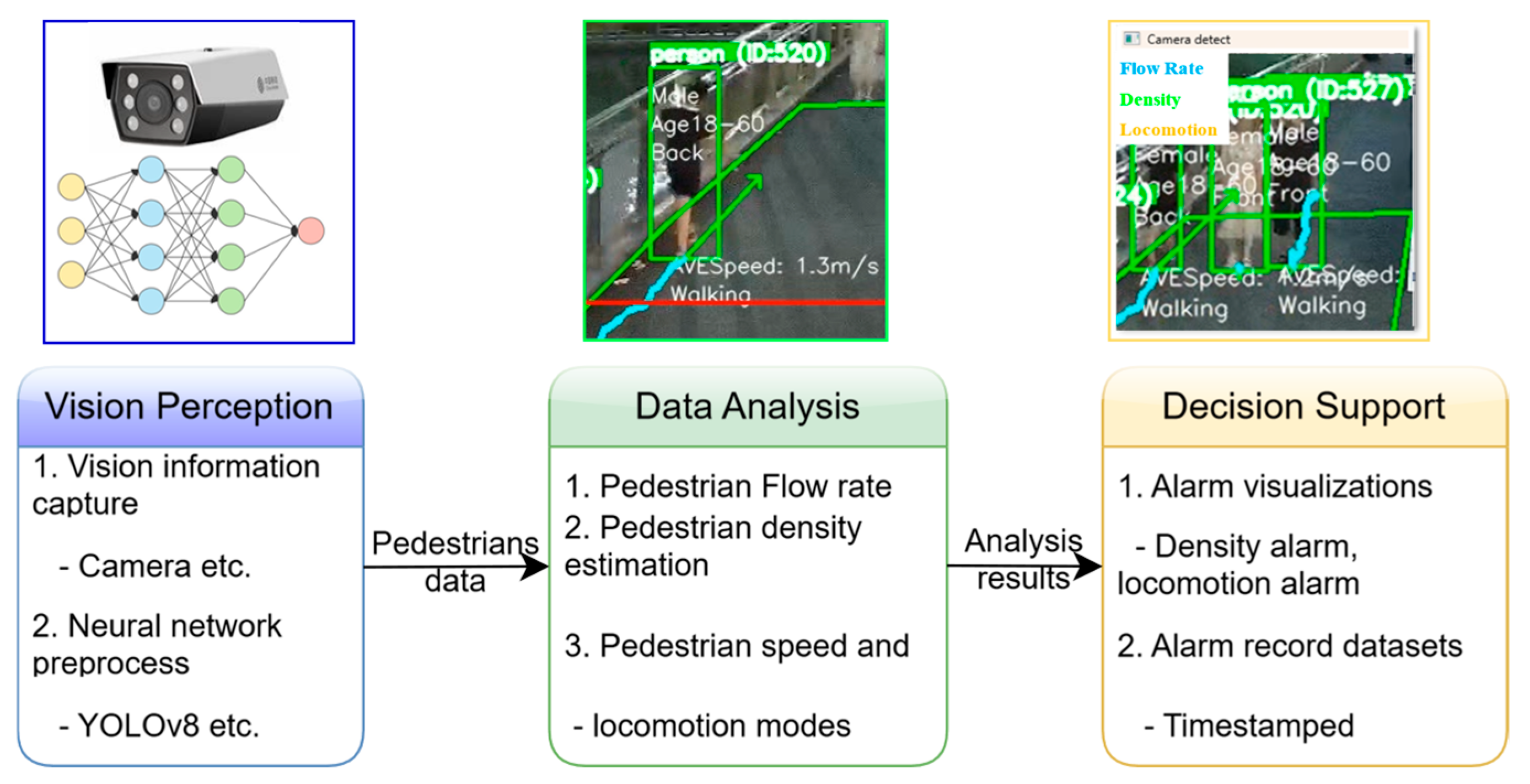
Figure 1.
The pedestrian management system architecture. Vision Perception (capturing and preprocessing data), Data Analysis (calculating pedestrian flow, density, speed), and Decision Support (providing alarm visualizations and timestamped records for further actions). The colored circles in Vision Perception schematically represent different conceptual layers of the neural network processing pipeline.
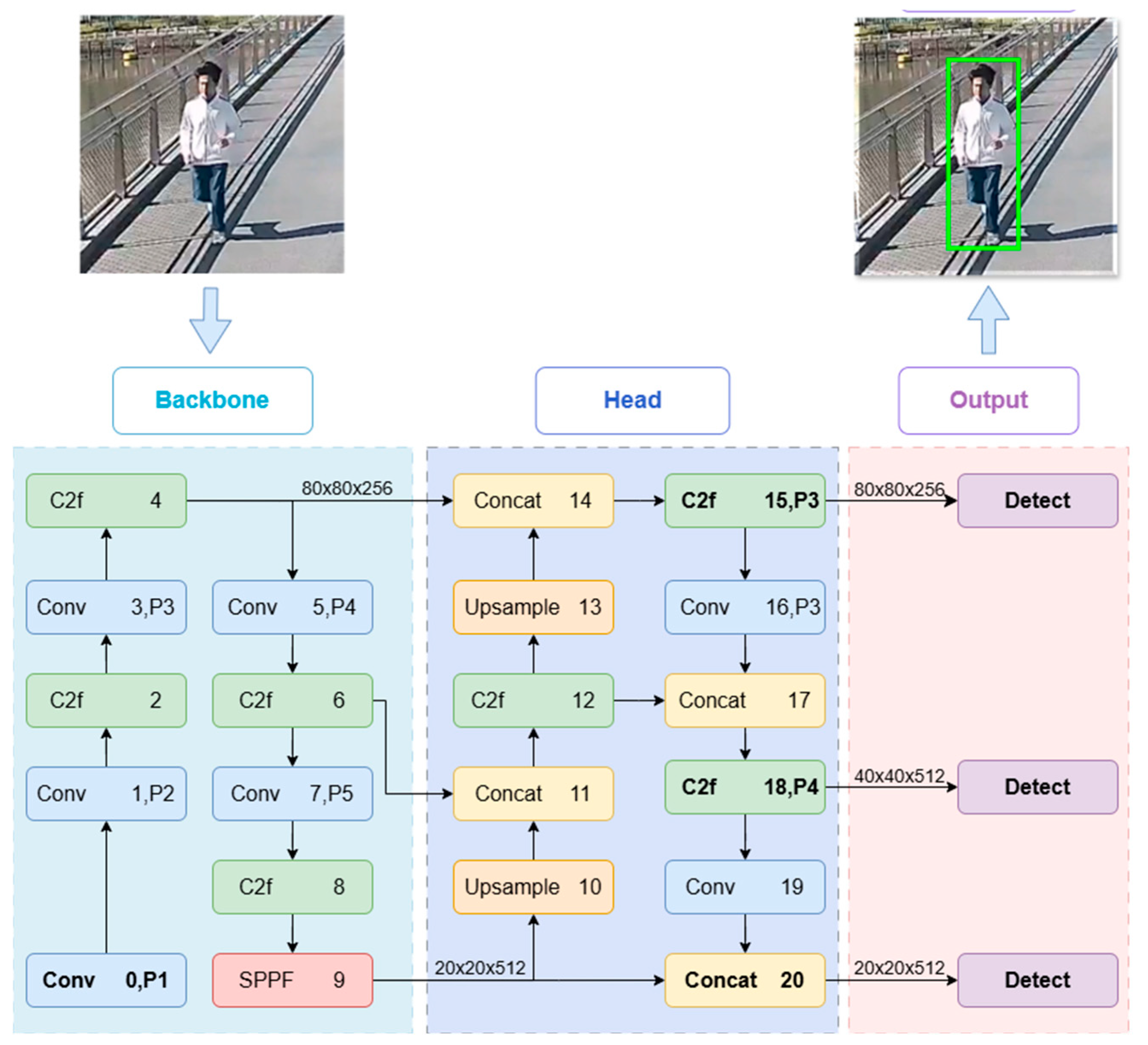
Figure 2.
YOLOv8 detect model structure. The backbone performs feature extraction through convolutional layers (Conv), while the head handles concatenation (Concat) and Upsample to refine the features.
Figure 2.
YOLOv8 detect model structure. The backbone performs feature extraction through convolutional layers (Conv), while the head handles concatenation (Concat) and Upsample to refine the features.
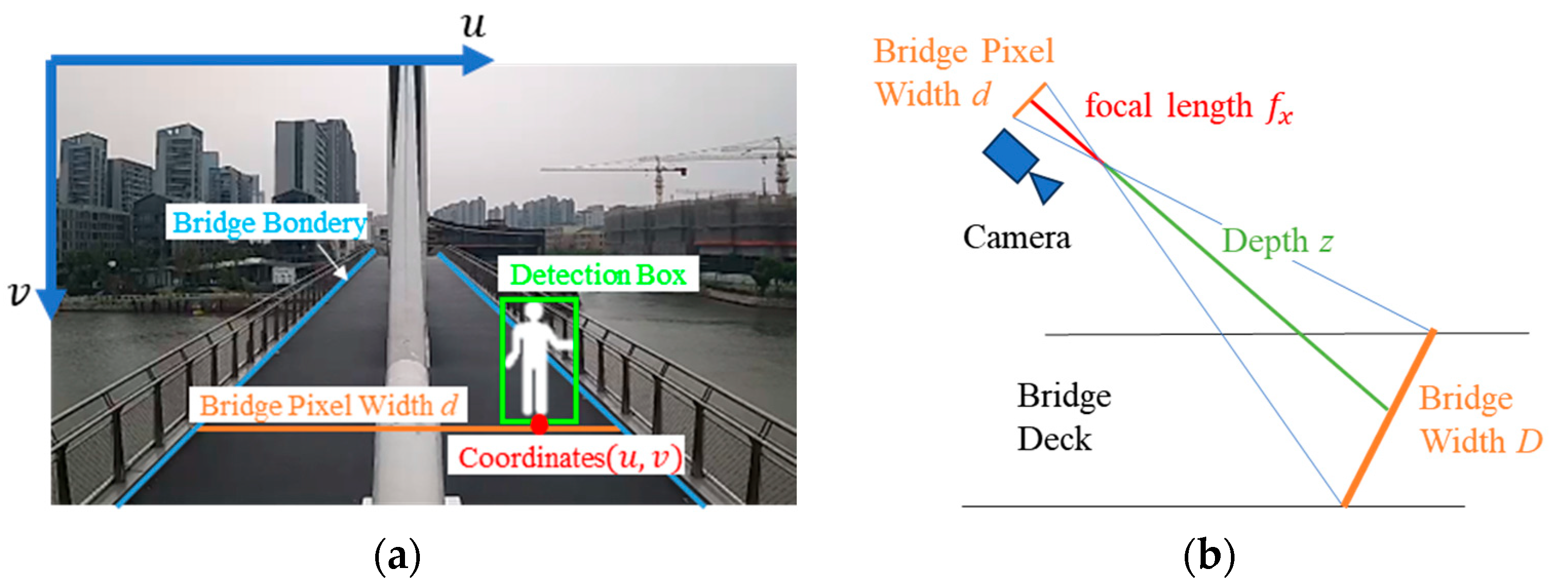
Figure 3.
Monocular Distance Measurement Diagram. (a) shows the key components such as the bridge’s boundary pixel width d, and the coordinates (u, v) of the detected pedestrian within the image. (b) shows the relationship between the bridge’s pixel width (d) and the actual bridge width (D). Focal length (fx) of the camera and the depth (z) are used to calculate the real-world distance based on the captured image.
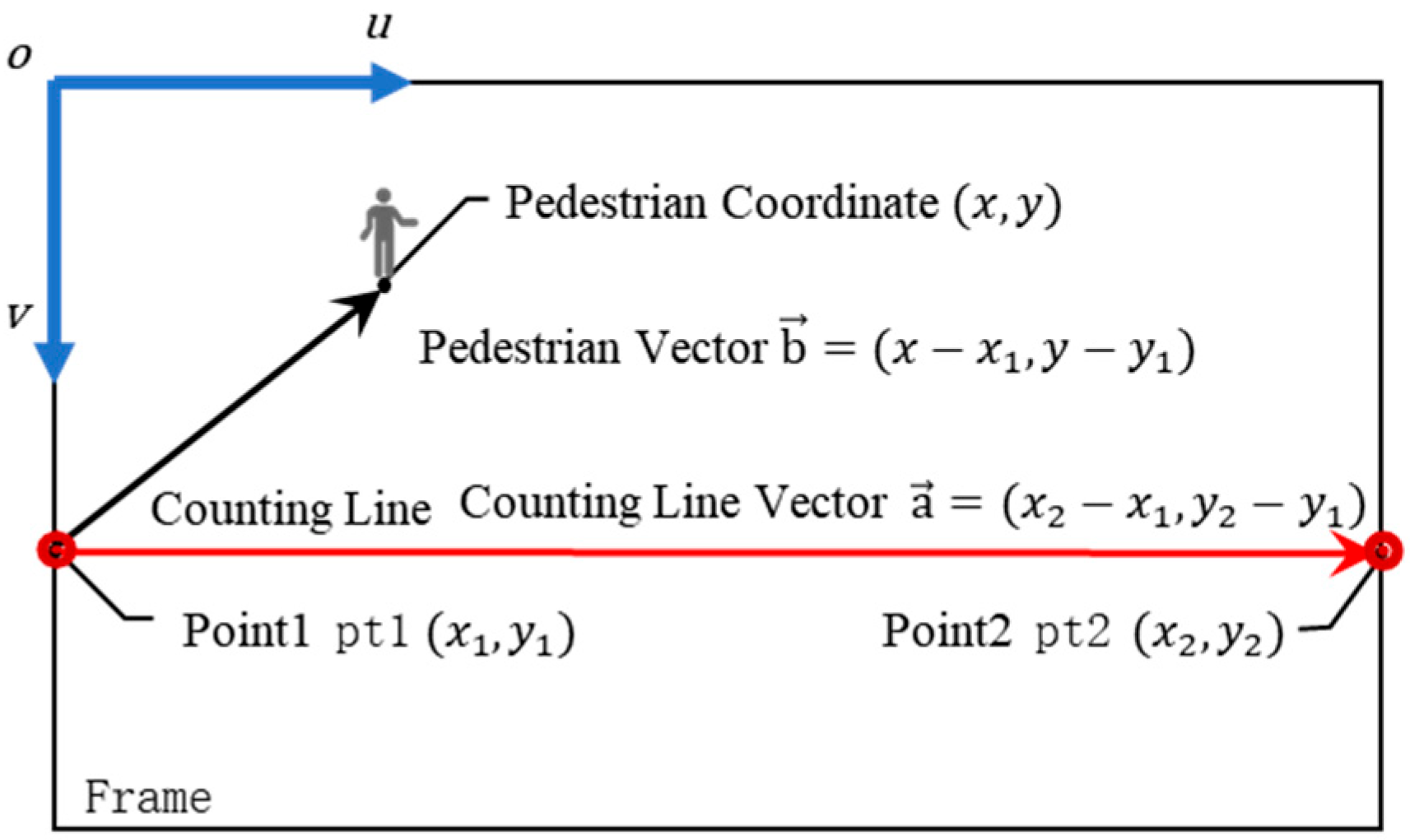
Figure 4.
Pedestrian counting using the vector cross product. In this setup, the pedestrian’s movement direction is represented by a black vector, while the red vector represents the counting line.
Figure 4.
Pedestrian counting using the vector cross product. In this setup, the pedestrian’s movement direction is represented by a black vector, while the red vector represents the counting line.
Figure 5.
The visualization of pedestrian flow count, density estimations, speed calculation and traffic alarms. (a) depicts a bidirectional counting system with the counting line marked in red. It tracks pedestrians moving in both directions. (b) shows a “crowded” density, leading to a “Crowded Traffic Alarm.” The green box represents the designated region of interest (ROI) for density measurement. (c) shows the “Running Tester” is being monitored by the system with the calculated speed and locomotion modes. The Chinese text in (b) refers to the original timestap from the experimental data and is integral to the raw dataset.
Figure 6.
Camera and Sensor Layout Diagram of the Pedestrian Bridge. The labels 1#–8# correspond to the bridge column numbers, from left to right.
Figure 6.
Camera and Sensor Layout Diagram of the Pedestrian Bridge. The labels 1#–8# correspond to the bridge column numbers, from left to right.
Figure 7.
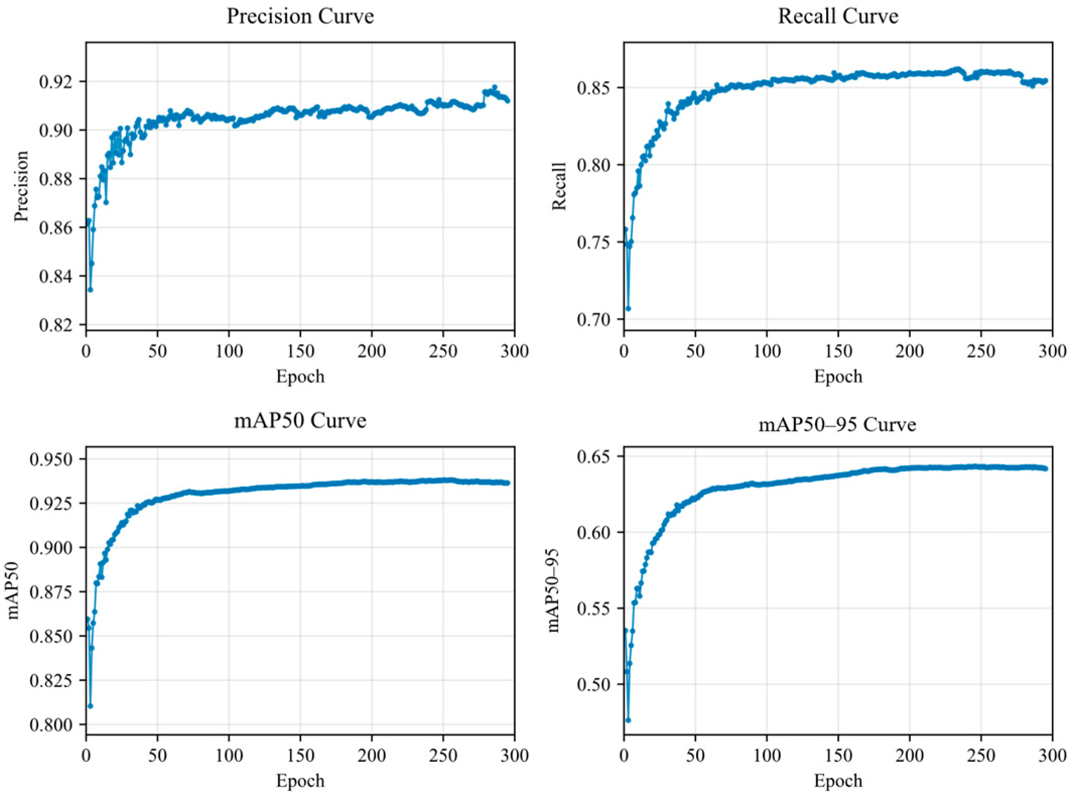
Training Results of YOLOv8n Model. Display four performance curves: Precision, Recall, mAP50, and mAP50–95 over 300 epochs.
Figure 7.
Training Results of YOLOv8n Model. Display four performance curves: Precision, Recall, mAP50, and mAP50–95 over 300 epochs.
Figure 8.
(a) Pedestrian position test with Laser Distance Meter and results with a scatter plot showing data points and the ideal line (represented by the red dashed line). The calculated distances all slightly above the actual distances, demonstrating the linear errors of the distance measurement system. (b) Corrected pedestrian position test results. The corrected data points are closely aligned with the ideal line, suggesting that the distance measurements have been effectively adjusted for accuracy.
Figure 9.
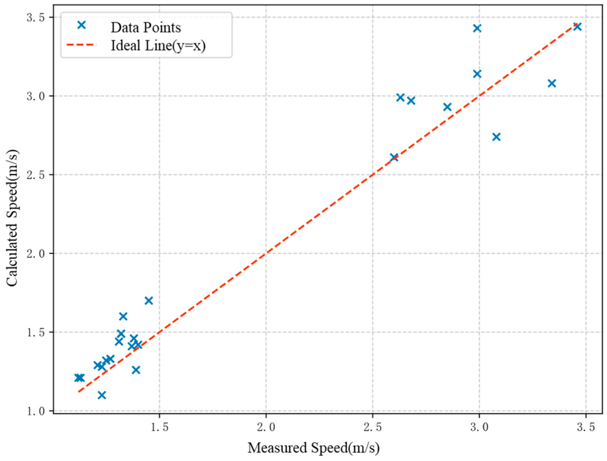
Displays the test results with a scatter plot comparing the measured speed versus the calculated speed. The data points generally follow the ideal line (represented by the dashed red line).
Figure 9.
Displays the test results with a scatter plot comparing the measured speed versus the calculated speed. The data points generally follow the ideal line (represented by the dashed red line).
Figure 10.
Two scenarios within the pedestrian flow management system, highlighting its early warning capabilities. (a) shows a “Busy in ROI” alarm triggered by the density of pedestrians within ROI. (b) shows a “Fast Running” alarm triggered by pedestrian moving rapidly through with a speed above 2.5 m/s. The Chinese text in figures refers to the original timestap from the experimental data and is integral to the raw dataset.
Figure 11.
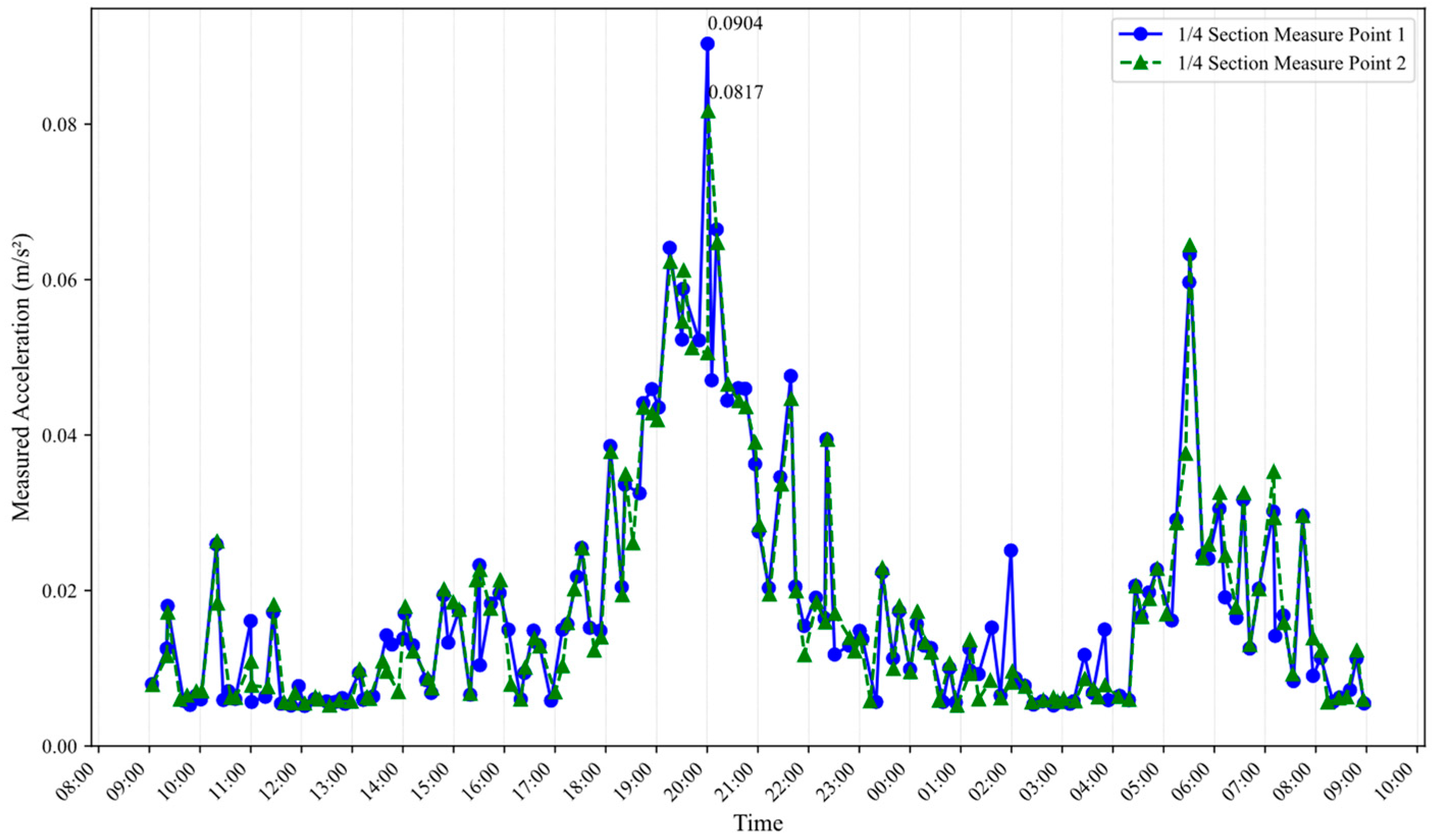
Measured acceleration of the 1/4 section of footbridge from 9:30 a.m. to 9:30 a.m. the Next Day. The peaks in acceleration appears with values reaching up to 0.0904 m/s2 around 8:00 p.m.
Figure 11.
Measured acceleration of the 1/4 section of footbridge from 9:30 a.m. to 9:30 a.m. the Next Day. The peaks in acceleration appears with values reaching up to 0.0904 m/s2 around 8:00 p.m.
Figure 12.
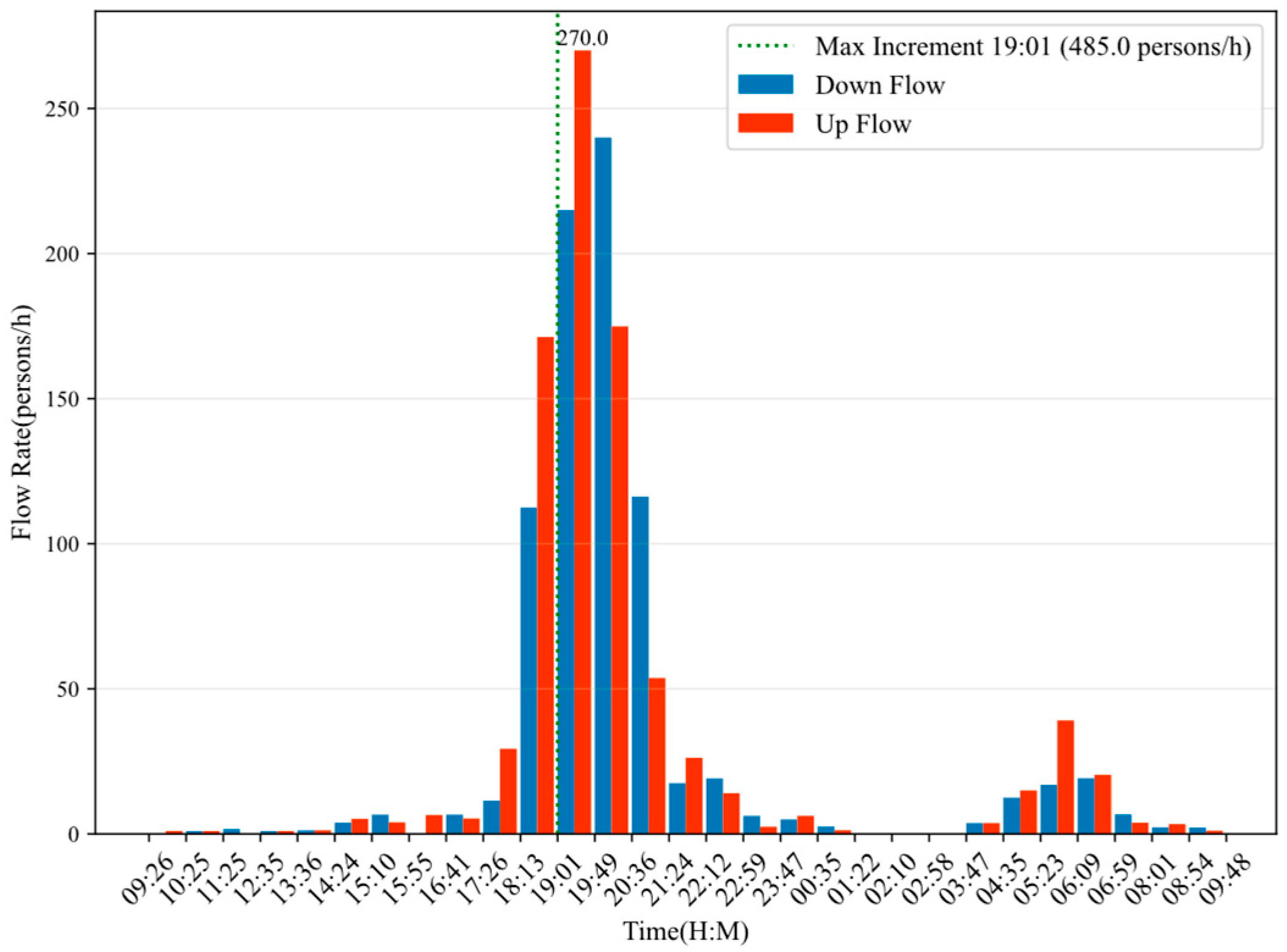
Pedestrian Flow Rate From 9:30 a.m. to 9:30 a.m. the Next Day. The flow rates for both “Down Flow” (blue bars) and “Up Flow” (red bars) measured in persons per hour. The maximum increment of 485 persons per hour occurred at 19:01, as indicated by the green dashed line.
Figure 12.
Pedestrian Flow Rate From 9:30 a.m. to 9:30 a.m. the Next Day. The flow rates for both “Down Flow” (blue bars) and “Up Flow” (red bars) measured in persons per hour. The maximum increment of 485 persons per hour occurred at 19:01, as indicated by the green dashed line.
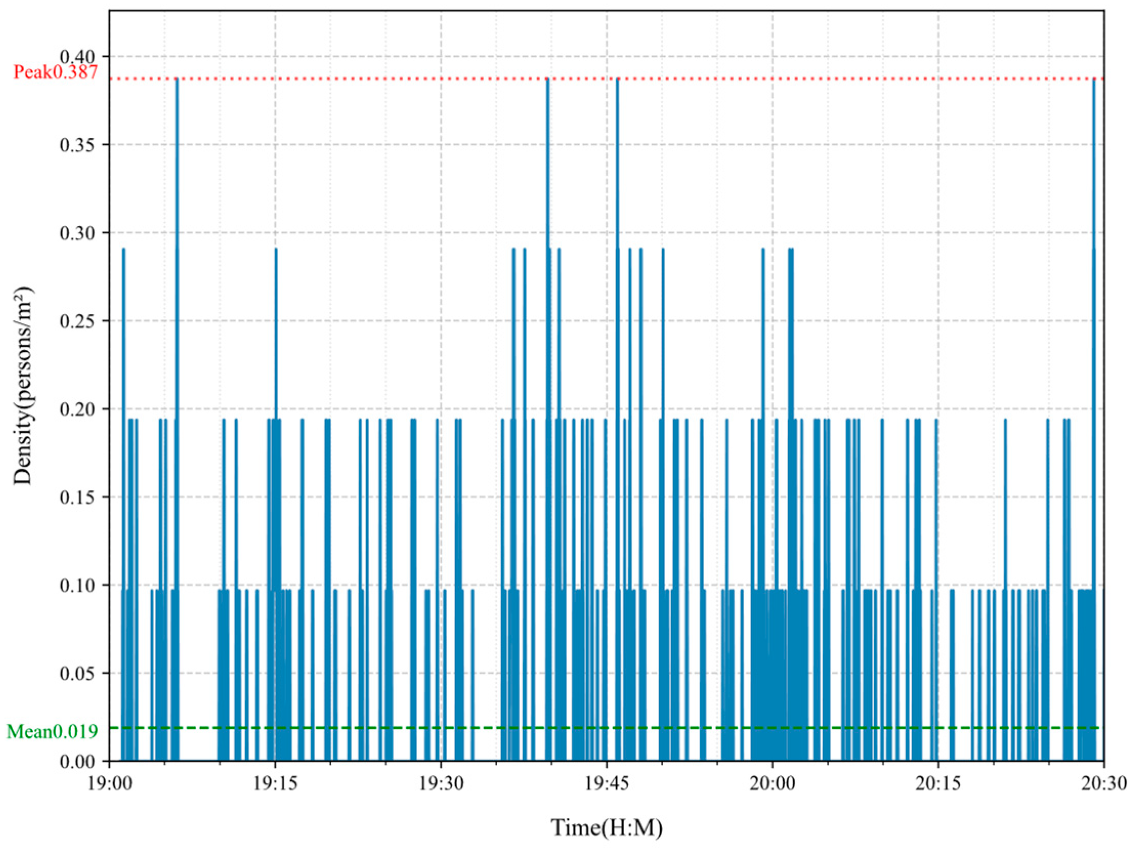
Figure 13.
Pedestrian Density From 7:00 p.m. to 8:30 p.m. during bridge operational hours. The red dashed line marks the peak density of 0.387 persons/m2, represents an observed instantaneous occurrence where 4 individuals are simultaneously present within a representative 10 m2 section of the target area. while the green line indicates the average density of 0.019 persons/m2.
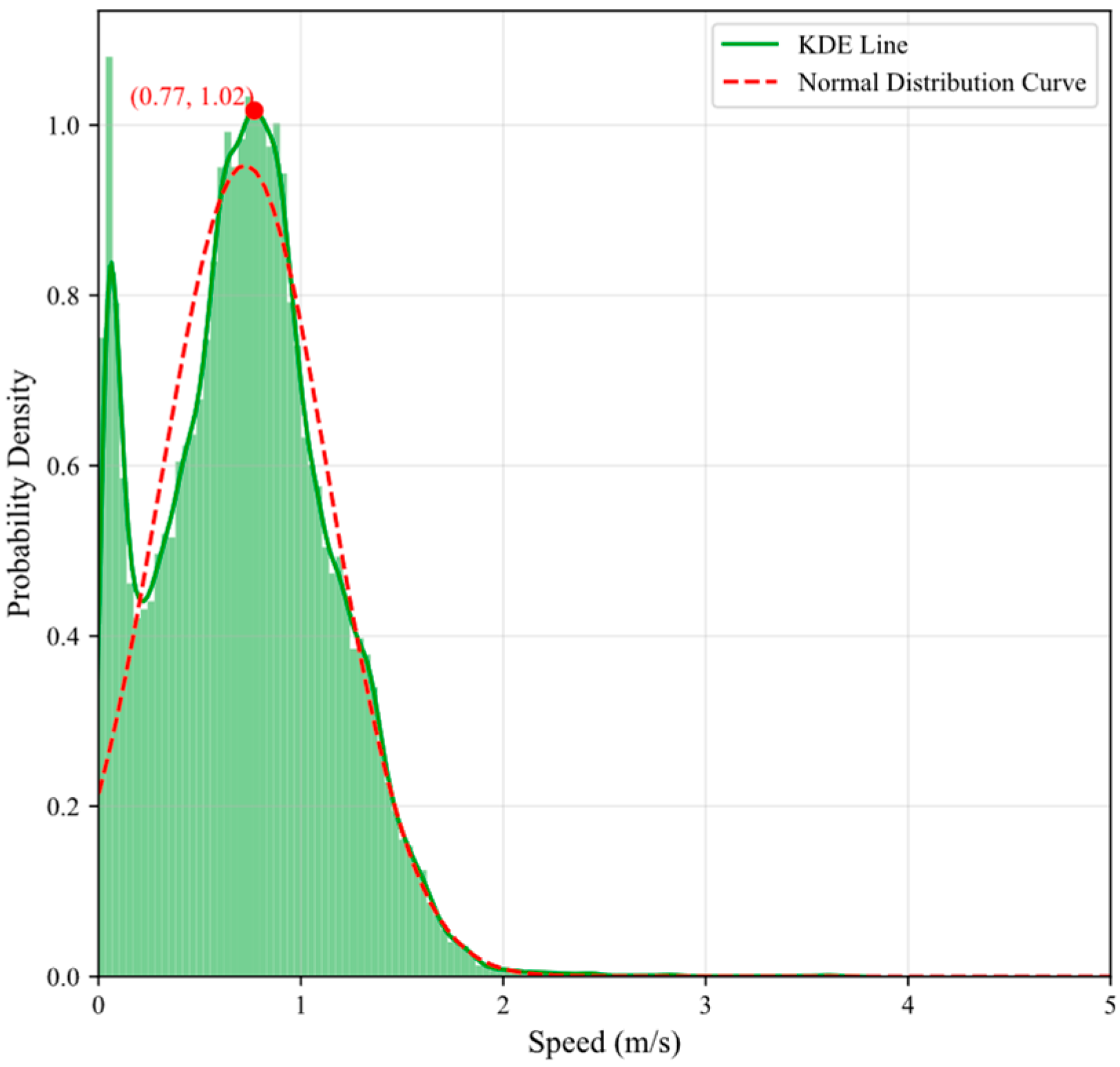
Figure 14.
The Probability Density Graph of Pedestrian Speeds. The green shaded area represents the Kernel Density Estimation (KDE) line, indicates that most pedestrians have a speed around 0.77 m/s, with a peak probability density of 1.02 m/s.
Figure 14.
The Probability Density Graph of Pedestrian Speeds. The green shaded area represents the Kernel Density Estimation (KDE) line, indicates that most pedestrians have a speed around 0.77 m/s, with a peak probability density of 1.02 m/s.
Figure 15.
(a,b) exemplify cases where cyclists are misidentified as runners. These three cycling instances resulted in three false alarms.
Figure 15.
(a,b) exemplify cases where cyclists are misidentified as runners. These three cycling instances resulted in three false alarms.
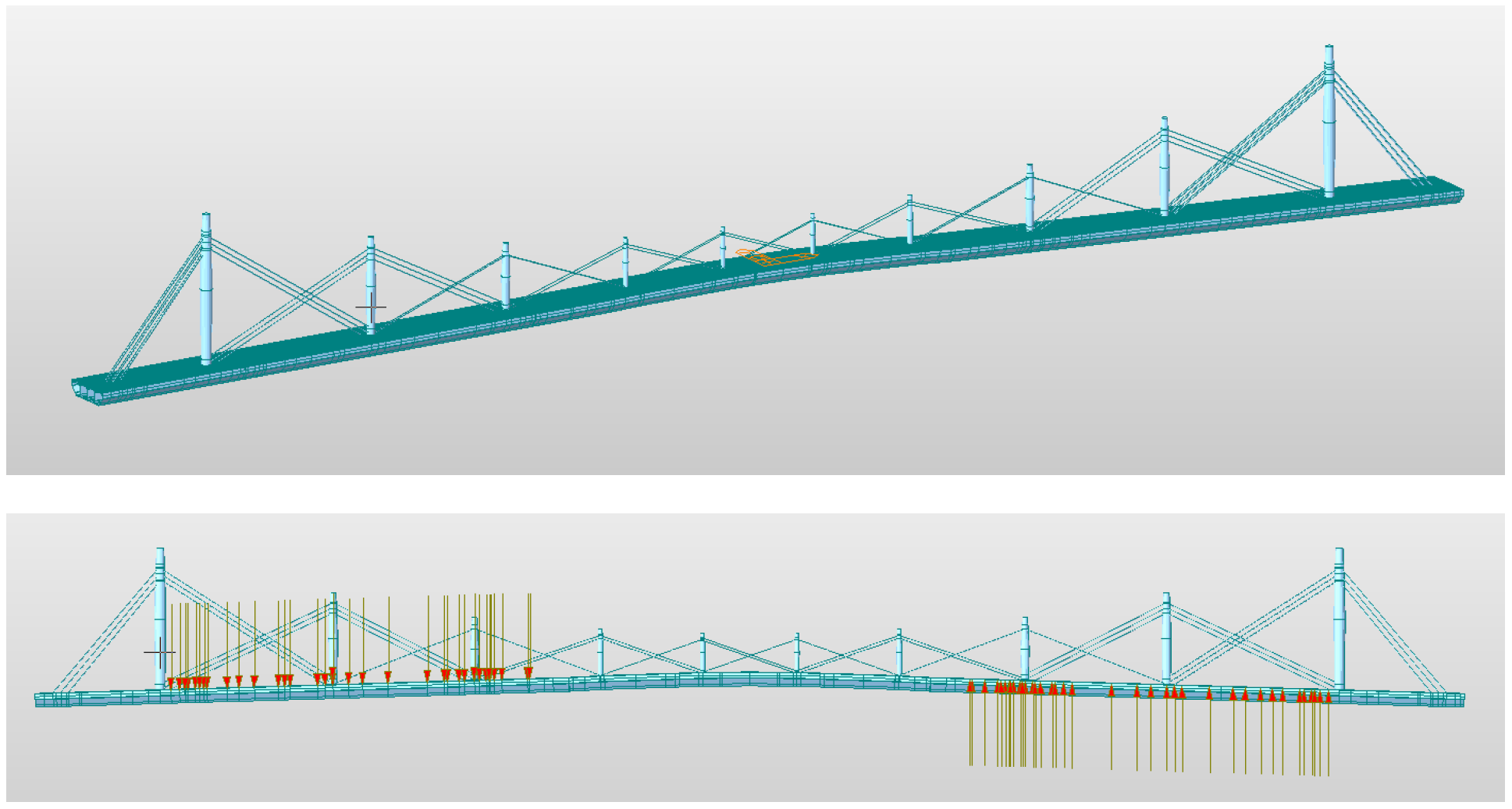
Figure 16.
The FEA model of a bridge, along with the measured pedestrian vertical loading method. The pedestrian load is converted from a uniformly distributed load to node loads, which are then proportionally distributed. Based on the mode shapes, the loads are applied in an anti-symmetric manner to the regions corresponding to the measured pedestrian density. Arrows show the direction and points where the external load is applied.
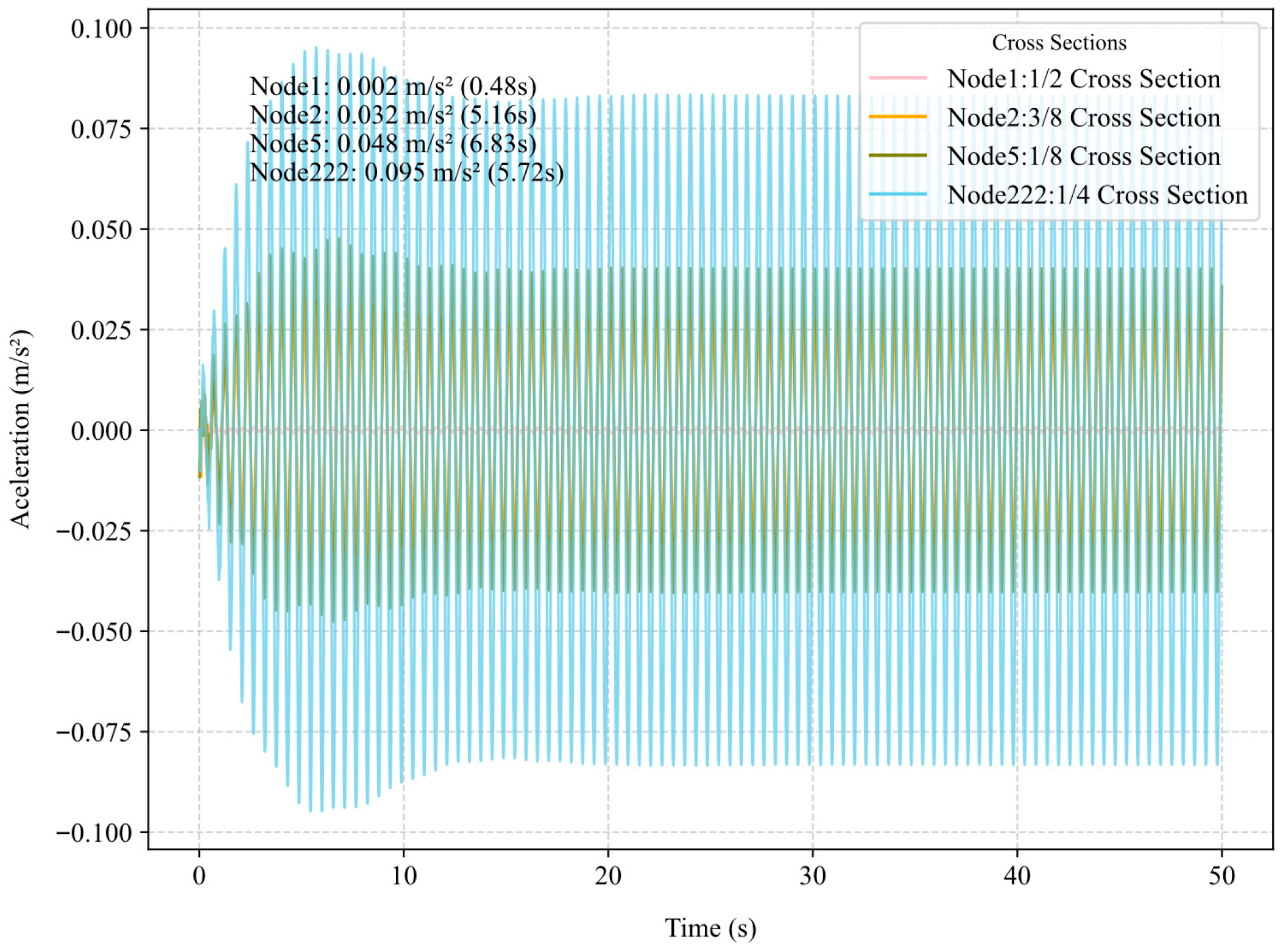
Figure 17.
The vertical vibration acceleration time history curve. The graph shows the acceleration values over time. These cross sections include 1/2, 3/8, 1/8, and 1/4. Each line represents the acceleration experienced at these points across the 50 s period.
Figure 17.
The vertical vibration acceleration time history curve. The graph shows the acceleration values over time. These cross sections include 1/2, 3/8, 1/8, and 1/4. Each line represents the acceleration experienced at these points across the 50 s period.
Table 1.
Pedestrian Density Level Classification.
Table 1.
Pedestrian Density Level Classification.
| Traffic Level | Description | Pedestrian Density (Persons/m2) |
|---|
| Level 1 | Sparse traffic | d < 0.5 |
| Level 2 | Busy traffic | 0.5 ≤ d ≤ 1.5 |
| Level 3 | Crowded traffic | d > 1.5 |
Table 2.
Technical Specifications of Video Surveillance Camera.
Table 2.
Technical Specifications of Video Surveillance Camera.
| Category | Specification |
|---|
| Sensor Type | 1/3″ Progressive Scan CMOS |
| Resolution | 1920 × 1080 (Full HD) |
| Frame Rate | 25 fps |
| Video Encoding | H.265/H.264 |
| Network Protocols | IPv4/IPv6, HTTP, DNS, NTP, RTP |
| Audio Input | Built-in microphone |
| Audio Output | Built-in speaker |
Table 3.
Technical Specifications of Triaxial Accelerometer.
Table 3.
Technical Specifications of Triaxial Accelerometer.
| Category | Specification |
|---|
| Measurement: | XYZ triaxial |
| Range: | ±2 g |
| Accuracy | ±1 mg |
| Operating Temperature | −20 to +65 °C |
| Frequency Response: | 0–200 Hz |
| Protection Rating | IP68 |
| Protective Cover | Material Steel |
| Signal Cable | RS485 digital interface |
Table 4.
300th training results of different datasets.
Table 4.
300th training results of different datasets.
| Training Datasets | P | R | mAP50 | mAP@50–95 |
|---|
| Combined dataset | 0.911 | 0.857 | 0.937 | 0.643 |
| CUHK | 0.888 | 0.767 | 0.849 | 0.613 |
Table 5.
Performance Comparison of Different Models on the CrowdHuman Validation Dataset.
Table 5.
Performance Comparison of Different Models on the CrowdHuman Validation Dataset.
| Training Datasets | P | R | mAP50 | mAP@50–95 | Speed (it/s) |
|---|
| YOLOv8n | 0.652 | 0.438 | 0.509 | 0.251 | 10.06 |
| YOLOv8s | 0.656 | 0.469 | 0.528 | 0.264 | 7.21 |
| Combined-T-Model | 0.735 | 0.504 | 0.626 | 0.287 | 10.81 |
| CUHK-T-model | 0.762 | 0.490 | 0.606 | 0.268 | 7.94 |
Table 6.
Comparative Algorithmic vs. Manual Pedestrian Counts Across Bidirectional Scenarios.
Table 6.
Comparative Algorithmic vs. Manual Pedestrian Counts Across Bidirectional Scenarios.
| Number | Group | Direction | Actual Count
(Persons) | Estimated Count
(Persons) | Relative Accuracy |
|---|
| 1 | 15-person queue | Bottom to Top | 15 | 14 | 93.3% |
| 2 | 15-person queue | Top to Bottom | 15 | 15 | 100.0% |
| 3 | 30-person queue | Bottom to Top | 30 | 26 | 86.7% |
| 4 | 30-person queue | Top to Bottom | 30 | 29 | 96.7% |
| 5 | 30-person random | Bottom to Top | 30 | 27 | 90.0% |
| 6 | 30-person random | Top to Bottom | 30 | 29 | 96.7% |
Table 7.
Pedestrian density test with busy and crowded Scenarios.
Table 7.
Pedestrian density test with busy and crowded Scenarios.
| Number | Area (m2) | Actual Density (Persons/m2) | Calculated Density (Persons/m2) | Relative Error | Congestion Level |
|---|
| 1 | 4 | 0.75 | 0.7278 | 3.0% | Busy |
| 2 | 4 | 0.75 | 0.7536 | 0.5% | Busy |
| 3 | 4 | 1 | 0.9814 | 1.9% | Busy |
| 4 | 4 | 1 | 0.9724 | 2.8% | Busy |
| 5 | 2 | 1.5 | 1.503 | 0.2% | Crowded |
| 6 | 2 | 1.5 | 1.558 | 3.9% | Crowded |
Table 8.
Pedestrian speed data from 7:00 p.m. to 8:30 p.m.
Table 8.
Pedestrian speed data from 7:00 p.m. to 8:30 p.m.
| Statistical Factor | Value |
|---|
| Sample Size | 180,264 |
| Mean | 0.72 m/s |
| Standard Deviation | 0.42 m/s |
| Maximum Value | 3.68 m/s |
| 25% Percentile | 0.42 m/s |
| Median | 0.73 m/s |
| 75% Percentile | 0.99 m/s |
Table 9.
Pedestrian flow count result comparison.
Table 9.
Pedestrian flow count result comparison.
| Direction | System Count
(Persons) | Manual Count
(Persons) | Accuracy |
|---|
| Pedestrian Flow (Up) | 216 | 228 | 94.7% |
| Pedestrian Flow (Down) | 172 | 175 | 98.3% |
| Total Pedestrian Flow | 388 | 403 | 96.3% |
Table 10.
Finite Element Simulation vs. Field Measurement Comparison of Peak Acceleration.
Table 10.
Finite Element Simulation vs. Field Measurement Comparison of Peak Acceleration.
| Section Location | Data Source | Peak Acceleration (m/s2) |
|---|
| 1/2 Section | FEM Simulation | 0.002 |
| 3/8 Section | FEM Simulation | 0.032 |
| 1/8 Section | FEM Simulation | 0.048 |
| 1/4 Section | FEM Simulation | 0.095 |
| 1/4 Section | Field Measurement 1# | 0.081 |
| 1/4 Section | Field Measurement 2# | 0.090 |
