Numerical Simulation and Analysis of the Influencing Factors of Ice Formation on Electrified Railway Contact Lines

Abstract

This study focuses on the icing problem of electrified railway contact lines. Using computational fluid dynamic (CFD) numerical simulations, a three-dimensional mesh model of the CuAg0.1AC120 contact line was developed. This study reveals the effects of environmental factors such as droplet diameter, air–liquid water content (LWC), and ambient temperature on the icing morphology. The results show that the asymmetric cross-sectional structure of the contact line causes localized droplet accumulation in the groove areas, leading to distinctly non-uniform and directional ice formation. At high wind speeds, secondary icing is observed on the leeward side, where droplets are carried by bypass airflow—this phenomenon is not prominent in standard conductors. Additionally, the contact line exhibits a more sensitive response to temperature and air moisture content changes, suggesting that it is more suited to a localized anti-icing strategy. The numerical model developed in this study provides a theoretical foundation for predicting ice loads on complex section conductors and supports the design optimization and maintenance of high-speed railway catenary systems.

1. Introduction

The overhead contact line (OCL) system of electrified railways is a tensioned cable structure laid along the railroad tracks and is the only source of electric power for electric locomotives [1]. However, in actual operation, the contact line system is often affected by environmental factors such as strong winds, freezing rain, snow, and other extreme weather conditions [2,3]. Environmental loads can cause ice accumulation on the contact line, leading to changes in the geometry of the high-speed rail OCL. This not only impacts the current collection quality of high-speed trains but can also cause the occurrence of galloping phenomena [4,5]. According to a report by the Workers’ Daily, on 14 December 2023, the contact line in the Xinxiang Power Supply Section of the China Railway Zhengzhou Group Co., Ltd. was affected by heavy rain, snow, and strong winds and experienced multiple instances of galloping icing along the Xinyan Line, from the tower laying section to the Suanwangzhuang area. The contact line continued to gallop for 14 h, resulting in 235 instances of return lines being detached. In 2011, after icing occurred on a section of the Luoxiang Line, severe galloping occurred with an amplitude of up to 0.5 m, forcing two trains to stop operations. Therefore, to reduce the harm caused by icing on the OCL system and ensure the safety of people’s lives and property, studying icing on contact lines is of significant importance.

When the ambient temperature is below freezing, a large number of water droplets remain in an unstable liquid state. When subjected to vibration, these droplets can crystallize. This unstable liquid, which exists in the air at sub-zero temperatures, is referred to as supercooled water droplets. During the airflow process, these droplets collide with the OCL system. Upon collision, the droplet surface deforms, causing a decrease in the curvature and a reduction in the surface tension. The contact line itself can act as a condensation nucleus, promoting the condensation of supercooled water droplets into ice. In general, the formation of ice coverage on the contact line requires three essential conditions: the air temperature and the contact line surface temperature must both be at or below 0 °C; the relative humidity of the air must be 85% or higher; and the wind speed must exceed 1 m/s.

The icing of the OCL is influenced by various factors, making it highly uncertain. Currently, both domestic and international scholars have conducted a series of studies on OCL icing. Regarding the icing mechanism, Makkonen et al. [6] conducted an in-depth investigation of early research on conductor icing issues and provided detailed descriptions of related computational models. Their proposed icing theory model suggests that the collision coefficient, adhesion coefficient, and freezing coefficient of water droplets are the three key factors influencing the rate of ice accumulation. Jiang et al. [7] focused on the dry and wet icing growth process on insulators, exploring the critical conditions for dry and wet icing. By deriving formulae for the freezing time of water droplets and the collision interval of water droplets, they proposed a parametric description of the insulator icing types and confirmed that conductor icing is a process involving heat transfer, exchange, and balance. Tabakova et al. [8] developed a model for the solidification and cooling process of supercooled droplets, including spherical, truncated spherical, and experimental shapes, after colliding with a cold solid substrate. They proposed an analytical function based on undercooling, thermal resistance, and expansion parameters. Prodi et al. [9] analyzed the shape, internal structure, crystallization characteristics, and local density distribution of ice accumulation by comparing icing accumulation on fixed and rotating cylinders. Their study provided valuable data for understanding the icing mechanism and its practical applications. Fumoto et al. [10] experimentally studied the critical heat flux for icing on horizontal wires under cold airflow and water mist conditions, examining the effects of the wire diameter and droplet morphology on the critical heat flux. Lu et al. [11,12], through simulations of freezing rain processes under natural outdoor conditions and wind tunnel experiments, studied the growth process of ice on conductors, revealing the relationship between ice weight and climate conditions. Zhao et al. [13] conducted wind tunnel experiments on the thawing of different ice thicknesses using a high-speed train bogie as the research subject and established the relationship between melting energy consumption and melting power. Wang et al. [14,15] enhanced the performance and stability of active pantograph control systems using reinforcement learning, providing theoretical support for OCL structural design.

In terms of icing growth characteristics, Savadjiev and Jiang et al. [16,17] developed mathematical and physical models to optimize the prediction of the icing process and de-icing effects. They analyzed the impact of factors such as temperature, wind speed, current density, and ice thickness on the icing or de-icing processes and validated the accuracy and practicality of the models through experiments. Yang et al. [18] proposed a method to calculate the freezing fraction and collision coefficient and combined an empirical formula for the liquid water content for computation based on ice surface temperature and the ice mass growth rate. The study also introduced a method for measuring the ice mass growth rate based on online monitoring data and icing experimental measurements. Feng et al. [19,20] established a two-dimensional icing model for transmission lines, using Fluent software to calculate airflow fields and convective heat transfer. Their study considered the effects of factors such as wind speed, droplet median volume diameter, temperature, liquid water content, wind direction angle, and electric field strength on icing characteristics, with a particular focus on the impact of transmission line vibrations on icing. The results provide a useful reference for mitigating the effects of icing under different meteorological conditions, offering strong specificity and practicality. Guo et al. [21] treated the aerodynamic forces of the icing suspension system as a quasi-steady-state and used Fluent software to calculate the aerodynamic coefficients of the quasi-steady-state system. They also developed a dynamic model of the icing suspension system under crosswind conditions. By applying the Galerkin method, they converted the partial differential vibration equation into ordinary differential equations for numerical solutions. The results confirmed the consistency between the simulation and theoretical stability analysis, revealing the oscillation characteristics of the icing suspension system under crosswind conditions. Sadov et al. [22] studied the formation and melting of ice and snow on high-voltage power lines under ice storm conditions. Through mathematical modeling, they simulated the effect of applying high currents on the melting of ice layers on transmission lines. The model was applied to a concentric circular cross-section scenario and was used to determine the relationship between the ice layer melting time and increasing current intensity.

In terms of predicting the state of icing, Li et al. [23] proposed a method for predicting conductor icing based on numerical models and deep learning processes, aiming to explore the impact of complex environmental factors on the icing process. This method provides a theoretical foundation for giving early warnings about icing, de-icing strategy selection, and the study of oscillations triggered by icing in transmission line systems. Wang et al. [24] introduced a hybrid model to predict the short-term icing thickness of transmission lines. They developed a component prediction model for icing thickness based on feature selection and CGWO-ELM, which demonstrated good predictive performance and could improve prediction accuracy through Random Forest (RF) feature selection. Peter et al. [25,26] studied the icing issue on the overhead contact lines of electrified railroads, analyzing the impact of various meteorological conditions on icing thickness and determining the corresponding maximum icing thickness, offering a high reference value. Snaiki et al. [27] proposed an ice-to-liquid ratio (ILR) prediction method based on a feedforward neural network (FFNN) and metaheuristic optimization algorithms to improve the accuracy of transmission line icing prediction. Through global sensitivity analysis, they identified precipitation, temperature, dew point temperature, and wind speed as the main influencing factors, with the optimized FFNN model outperforming the traditional stochastic gradient descent method. Meng et al. [28] proposed a regional overhead transmission line framework under a combined wind–ice action based on meteorological station data and time series prediction models. They calculated and analyzed the impact of climate change on the vulnerability and failure probability of transmission lines and recommended supplementary design strategies to address climate change. Wang et al. [29,30] proposed a prediction model to improve the accuracy of existing transmission line icing prediction models and address the issue of ignoring the objective laws of icing. This model, based on Convolutional Neural Networks (CNNs) and Bidirectional Gated Recurrent Units (BiGRU), incorporates a weighted fusion of Soft Dynamic Time Warping (Soft-DTW) and icing change rules. This significantly enhances prediction accuracy and outperforms traditional non-mechanical models with smaller errors.

This paper takes the CuAg0.1AC120 model overhead contact line as the research object and uses computational fluid dynamic (CFD) numerical simulation methods to analyze the icing formation mechanism based on Fluent software. Additionally, to ensure the reliability of the simulation results, a validation analysis is performed by comparing the icing process of transmission conductors. The icing process of the contact line involves many complex factors, such as the wind direction relative to the groove and the possibility of conductor twisting or oscillation, which require deeper structural dynamics analysis. Given the limitations of computational resources and the focus of the research objectives, we chose basic variables such as the droplet diameter, air–liquid water content, and ambient temperature to develop the model, aiming to reveal their effects on the icing morphology. The research findings provide theoretical support for the safe operation of high-speed trains and offer an important scientific basis for the development of anti-icing and de-icing technologies for the overhead contact network.

2. Calculation and Simulation of Basic Parameters of Iced Contact Line

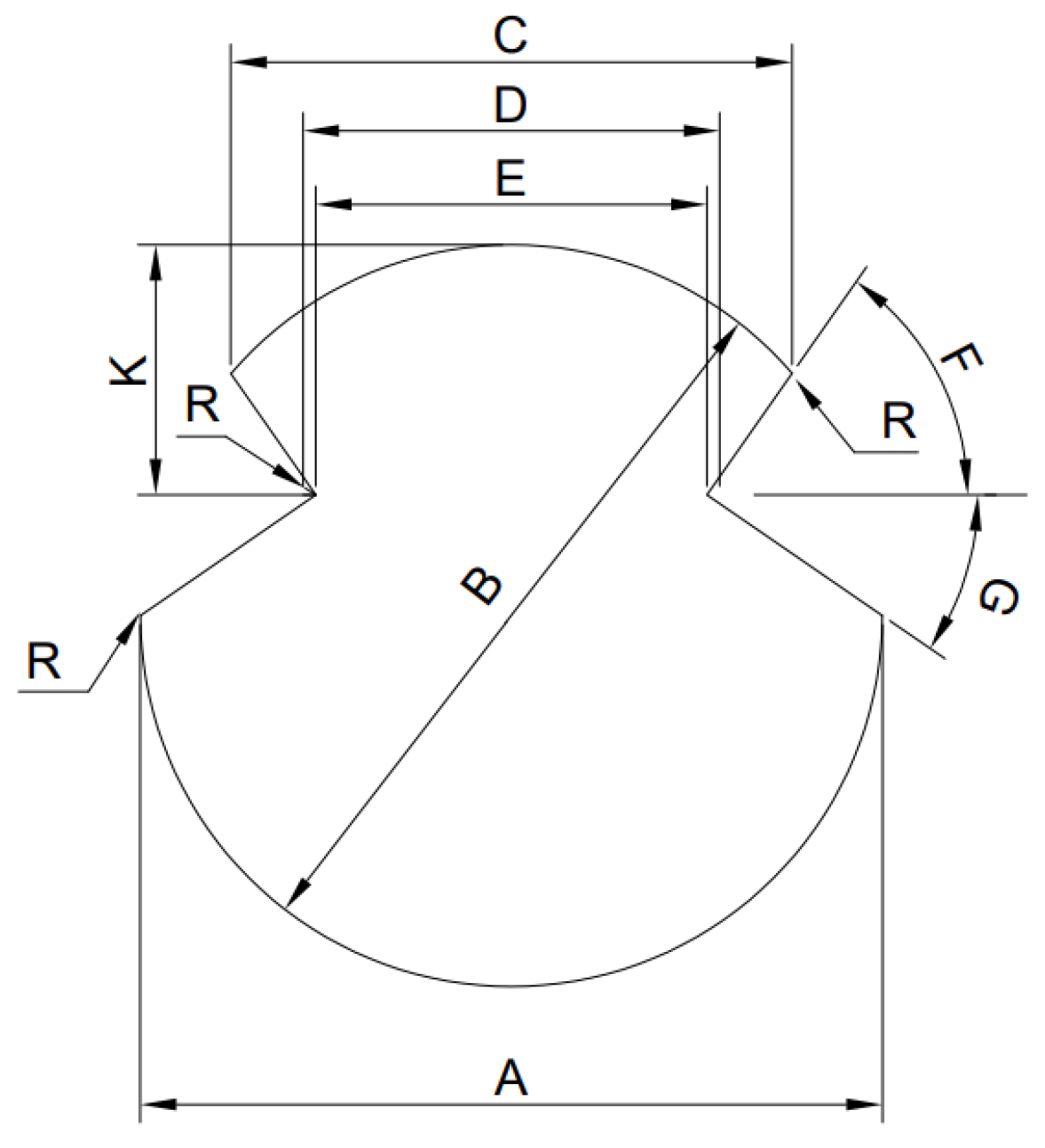
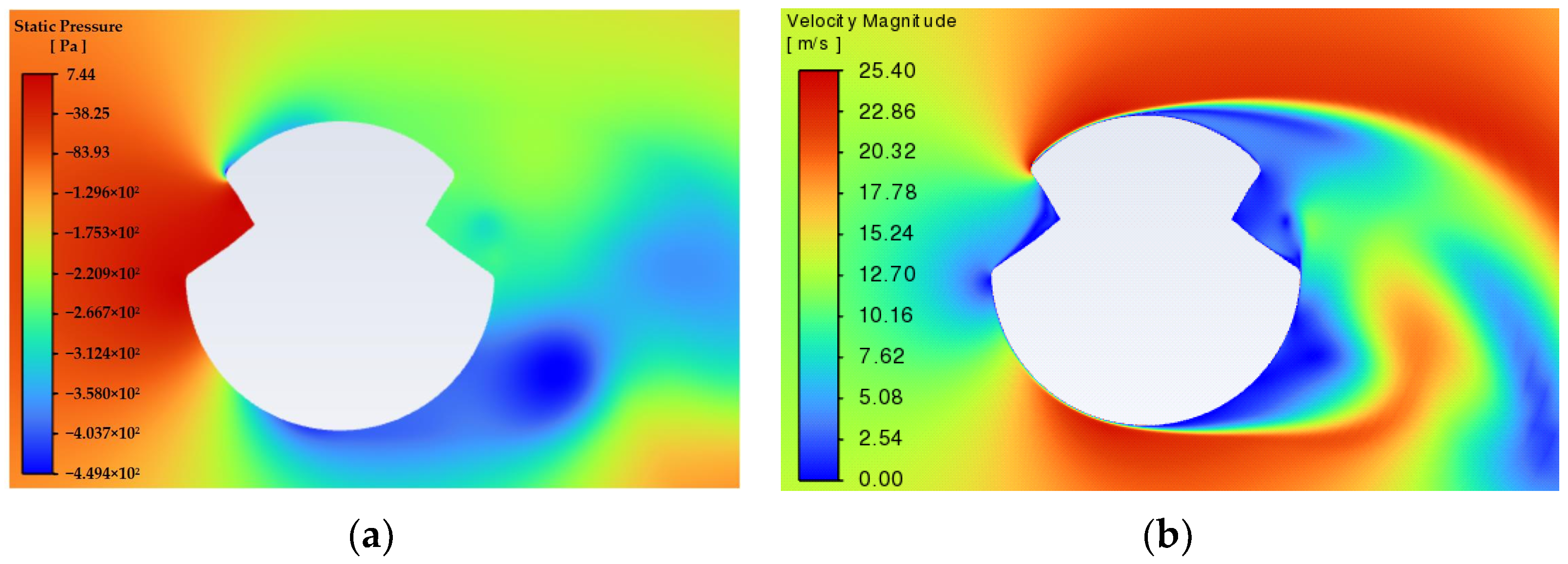
2.1. Establishment of the Fluid Calculation Domain

The study focuses on the CuAg0.1AC120 model overhead contact line, as shown in Figure 1, with specific parameters provided in

Table 1. Parameters of CuAg0.1AC120-type contact line.

Nominal	Calculation	Size (mm)							Angle (°)
Area (mm2)	Area (mm2)	A	B	C	D	E	K	R	F	G
120	121	12.9	12.9	9.76	7.24	6.8	4.35	0.4	51	27

. The computational domain is defined as a cylindrical region with a radius of 300 mm and a thickness of 100 mm. A structured grid is used for meshing, with a total grid size of approximately 3 million cells. To meet the condition of a wall y+ [31] value less than one, the height of the first mesh layer on the contact line’s surface is set to 0.04 mm, and the boundary layer mesh has a growth rate of 1.1. The boundary of the flow domain is defined as a wind speed inlet (Velocity_inlet), while the contact line boundary is defined as a no-slip wall (Wall). The model solver selected is a pressure-based solver, and the SST k-ω turbulence model is used to simulate the incompressible fluid around the contact line. The SST k-ω turbulence model is commonly used to simulate flow near the walls and performs better than the k-ε turbulence model in handling strong curvature, internal flows, and separated flows, especially when simulating icing processes, as it accurately captures boundary layer behavior. The SIMPLEC algorithm is used to address the coupling between velocity components and pressure. Figure 2 shows the mesh of the flow domain surrounding the contact line CFD model, where Figure 2a presents the mesh for the entire flow domain, and Figure 2b provides a zoomed-in view of the contact line region, with higher mesh quality being closer to the contact line’s cross-section.

The boundary conditions are set, and the relevant parameters are specified. For the SST k-ω model, the calculation methods for the turbulence parameters are as follows:

$$\left\{\begin{array}{c}I=0.16R{e}^{-\frac{1}{8}}\\ k=1.5{(\overline{u}I)}^2\\ w=\mathsf{\rho }{C}_{\mathsf{\mu }}{k}^2/{\mathsf{\mu }}_t\end{array}\right.$$

(1)

where I is the turbulence intensity; k is the turbulent kinetic energy; Re is the Reynolds number; $\overline{u}$ is the average flow velocity; w is the turbulence frequency; $\mathsf{\rho }$ is the fluid density; ${\mathsf{\mu }}_t$ is the turbulence viscosity; and $C_{\mathsf{\mu }}$ is the turbulence constant, typically taken as 0.09. The simulation conditions are set with a wind speed of 15 m/s and an angle of attack of 0°, and the airflow field distribution is shown in Figure 3.

Figure 3a shows the pressure field contour around the contact line, and Figure 3b shows the velocity field contour around the contact line. Due to the presence of the contact line’s tail groove, there is a missing arc wall surface in the flow direction at the center of the contact line’s cross-section. As a result, after the airflow is compressed at the top of the cross-section, the flow velocity is lower than that at the lower-left side, causing the pressure above to be higher than the pressure below. When droplets move from the left side of the contact line to the right side, the velocity at the upper and lower boundaries is at a maximum, and the pressure is at a minimum.

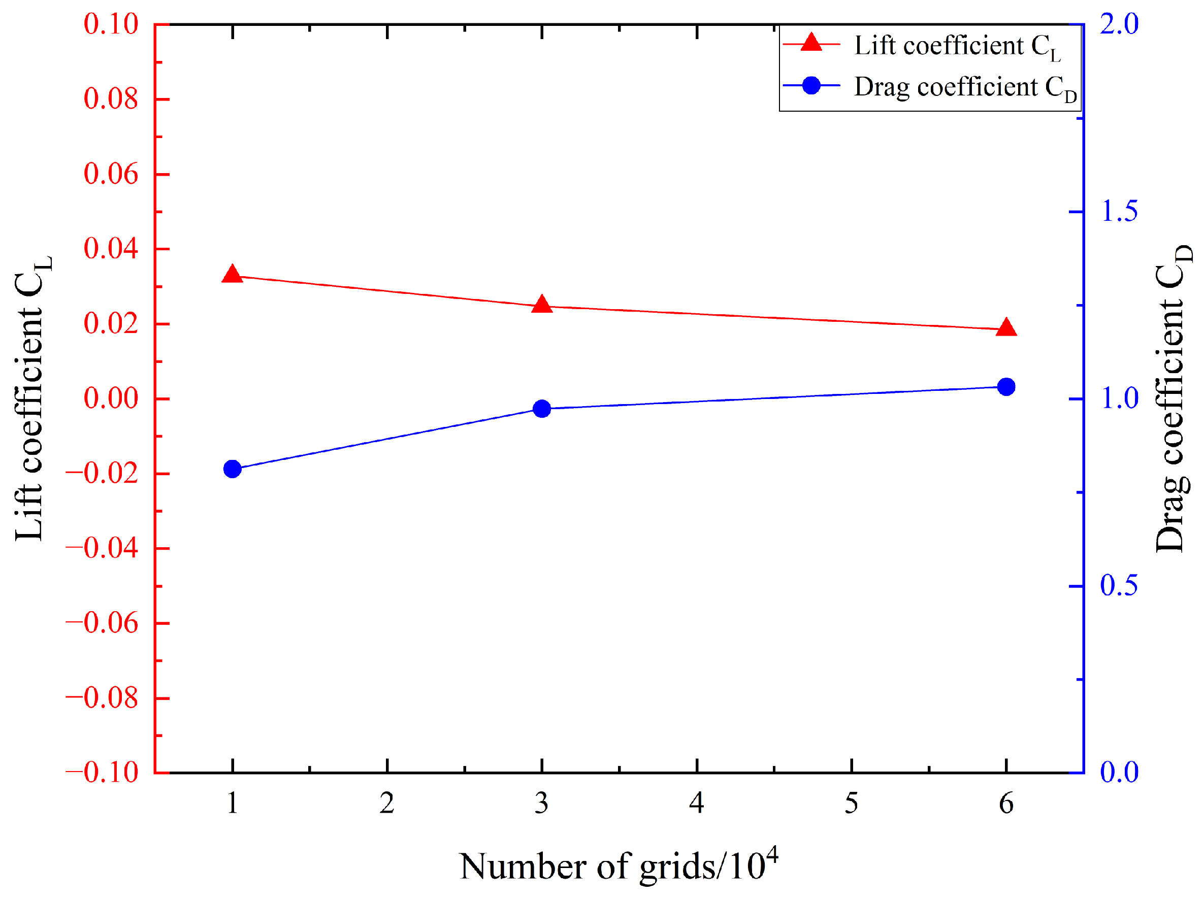
2.2. Mesh-Independent Verification

To validate the effectiveness of the grid model, mesh independence was verified by calculating the necessary aerodynamic coefficients in the icing simulation. With the wind speed set at 15 m/s and other conditions kept constant, flow domain models with different grid densities were created to verify the grid’s independence. Figure 4 shows the lift and drag coefficients of the contact line at different grid densities. The results indicate that further refinement of the grid has less than a ±0.05 impact on the results. The simulation results remain stable with minimal variation, so the current grid density was chosen to balance computational accuracy and efficiency.

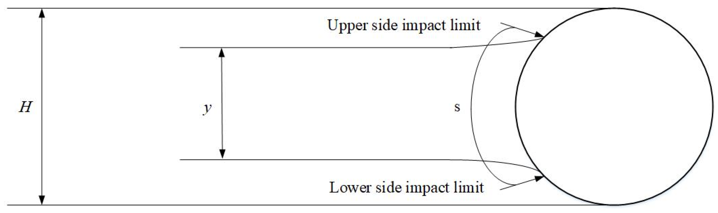
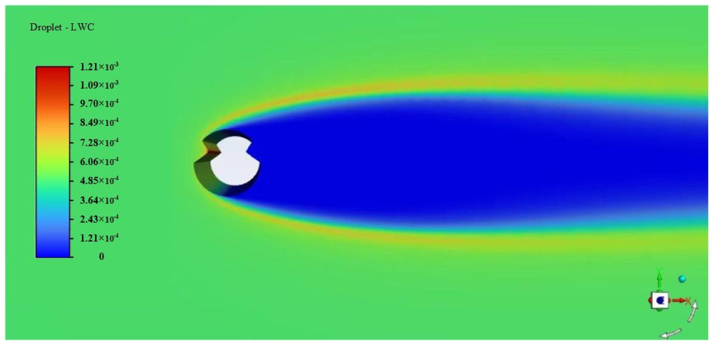
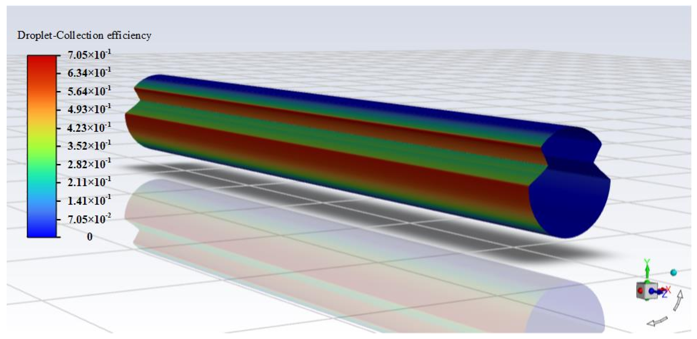
2.3. Study of Droplet Collision in the Overhead Contact Line System

Overhead contact line icing is a random physical phenomenon caused by the collision, capture, and freezing process of supercooled water droplets in the airflow. The Makkonen model [32] is generally used to study the characteristics and mechanisms of icing, and this is expressed as follows:

$${\displaystyle \frac{dM}{dt}}={\mathsf{\alpha }}_1{\mathsf{\alpha }}_2{\mathsf{\alpha }}_3\nu \mathsf{\varpi }A$$

(2)

In the equation, v represents the wind speed; $\mathsf{\varpi }$ is the liquid water content in the air; A is the effective area of the windward surface of the contact line; ${\mathsf{\alpha }}_1$ is the collision rate, which represents the probability of a droplet colliding with the surface of an object and is related to airspeed, droplet diameter, and object shape; ${\mathsf{\alpha }}_2$ is the capture rate, which represents the probability that a droplet colliding with the surface is captured, mainly influenced by surface roughness and wettability; and ${\mathsf{\alpha }}_3$ is the freezing rate, which represents the proportion of captured droplets that freeze into ice, and is related to ambient temperature and droplet supercooling.

To better understand the collision characteristics of water droplets, the local collision rate and overall collision rate are introduced. As shown in Figure 5, it is assumed that the water droplets within the incoming flow range H are carried toward the conductor along the flow direction. However, most of the water droplets are influenced by aerodynamic drag and are deflected around the conductor, following the flow field. As a result, the droplets that collide with the conductor all come from the droplets within range y. When droplets collide with the conductor, two distinct trajectories are formed on both the upper and lower sides of the conductor in tangent to the conductor’s surface. These two trajectories correspond to the droplets that collide with the conductor at extreme positions. The area enclosed by these two trajectories defines the collision zone of the droplets on the conductor.

The local collision rate $\beta$ is as follows:

$$\beta ={\displaystyle \frac{dy}{ds}}$$

(3)

In the equation, $dy$ represents the vertical distance between the trajectories of two water droplets in the initial airflow, and $ds$ is the distance between collision points on the iced surface. The value of $dy$ changes with the number of droplets tracked along the trajectories. For example, the highest number of droplets occurs at the stagnation point on the left side of the conductor, and as we move along both sides of the conductor from the stagnation point, the number of droplets gradually decreases until it reaches the collision limit, where the droplet count is zero.

The overall droplet collision rate ${\mathsf{\alpha }}_1$ is the ratio of the actual number of droplets colliding with the conductor surface per unit of time compared to the maximum possible number of droplets that could collide. The maximum possible droplet collision refers to the number of droplets that could strike the conductor surface without being deflected by the airflow. Based on this definition, the overall droplet collection coefficient can be expressed as follows:

$${\mathsf{\alpha }}_1={\displaystyle \frac{y}{H}}$$

(4)

According to the definition and formula, both ${\mathsf{\alpha }}_1$ and $\beta$ are dimensionless values that range from 0 to 1.

2.4. Droplet Trajectory Equation and Its Solution

To simulate the motion trajectories of droplets in the airflow, this study employed the Lagrange method to track the droplet phase, treating the droplets as a discrete phase. The motion of each droplet is tracked, and based on Newton’s second law, the droplet’s motion control equation is as follows:

$$m_{\mathrm{w}}{\displaystyle \frac{d^2{\overrightarrow{x}}_{\mathrm{w}}}{d{t}^2}}={\overline{F}}_1+{\overline{F}}_2={\displaystyle \frac{1}{2}}{\mathsf{\rho }}_{\mathrm{a}}{A}_{\mathrm{w}}{C}_{\mathrm{d}}\left|{\overrightarrow{u}}_{\mathrm{a}}-{\overrightarrow{u}}_{\mathrm{w}}\right|({\overrightarrow{u}}_{\mathrm{a}}-{\overrightarrow{u}}_{\mathrm{w}})+m_{\mathrm{w}}\overrightarrow{g}$$

(5)

In the equation, $m_{\mathrm{w}}$ represents the mass of the droplet; $x_{\mathrm{W}}$ is the displacement vector of the droplet; t is the time of droplet motion; $F_1$ is the drag force vector acting on the droplet; $F_2$ is the gravitational force vector acting on the droplet; ${\mathsf{\rho }}_{\mathrm{a}}$ is the air density (kg/m³); $A_{\mathrm{w}}$ is the frontal area of the droplet (m²); $C_{\mathrm{d}}$ is the drag coefficient of the droplet; $u_{\mathrm{a}}$ is the air velocity vector; and $u_{\mathrm{w}}$ is the velocity vector of the droplet.

The droplet’s frontal area $A_{\mathrm{w}}$ can be calculated using the following equation:

$$A_{\mathrm{w}}={\displaystyle \frac{4}{3}}\mathsf{\pi }{\mathsf{\rho }}_{\mathrm{w}}{\left({\displaystyle \frac{d_{\mathrm{w}}}{2}}\right)}^3={\displaystyle \frac{1}{6}}\mathsf{\pi }{\mathsf{\rho }}_{\mathrm{w}}{d}_{\mathrm{w}}^3$$

(6)

In this equation, ${\mathsf{\rho }}_{\mathrm{w}}$ represents the droplet density (kg/m³), and $d_{\mathrm{w}}$ represents the droplet diameter (m). Substituting Equation (6) into Equation (5) yields the following:

$${\displaystyle \frac{d^2{\overrightarrow{x}}_{\mathrm{w}}}{d{t}^2}}={\displaystyle \frac{18}{24}}{\displaystyle \frac{{\mathsf{\rho }}_{\mathrm{a}}{C}_{\mathrm{d}}}{{\mathsf{\rho }}_{\mathrm{w}}{d}_{\mathrm{w}}}}\left|{\overrightarrow{u}}_{\mathrm{a}}-{\overrightarrow{u}}_{\mathrm{w}}\right|({\overrightarrow{u}}_{\mathrm{a}}-{\overrightarrow{u}}_{\mathrm{w}})+\overrightarrow{g}$$

(7)

where the drag coefficient $C_{\mathrm{d}}$ can be calculated using the following formula [33]:

$$\left\{\begin{array}{c}{\displaystyle \frac{C_{\mathrm{d}}{R}_{\mathrm{c}}}{24}}=1+0.189\times R_{\mathrm{c}}^{0.632},21<R_{\mathrm{e}}\le 200\\ {\displaystyle \frac{C_{\mathrm{d}}{R}_{\mathrm{c}}}{24}}=1+0.115\times R_{\mathrm{c}}^{0.802},2<R_{\mathrm{e}}\le 21\\ {\displaystyle \frac{C_{\mathrm{d}}{R}_{\mathrm{c}}}{24}}=1+0.102\times R_{\mathrm{c}}^{0.955}, 0.2<R_{\mathrm{c}}<2\\ {\displaystyle \frac{C_{\mathrm{d}}{R}_{\mathrm{c}}}{24}}=1+0.197\times R_{\mathrm{c}}^{0.63}+2.6\times {\mathrm{e}}^{-4}\times R_{\mathrm{c}}^{1.38},R_{\mathrm{e}}<0.2 \mathrm{or} R_{\mathrm{e}}>200\end{array}\right.$$

(8)

Substituting Equation (8) into Equation (7) yields the following equation:

$$\left\{\begin{array}{c}{\displaystyle \frac{d{\overrightarrow{x}}_{\mathrm{w}}}{dt}}={\overrightarrow{u}}_{\mathrm{w}}\\ {\displaystyle \frac{d{\overrightarrow{u}}_{\mathrm{w}}}{dt}}+{\displaystyle \frac{18C_{\mathrm{d}}{R}_{\mathrm{e}}}{24}}{\displaystyle \frac{{\mathsf{\mu }}_{\mathrm{a}}}{{\mathsf{\rho }}_{\mathrm{w}}{d}_{\mathrm{w}}^2}}{\overrightarrow{u}}_{\mathrm{w}}={\displaystyle \frac{18C_{\mathrm{d}}{R}_{\mathrm{e}}}{24}}{\displaystyle \frac{{\mathsf{\mu }}_{\mathrm{a}}}{{\mathsf{\rho }}_{\mathrm{w}}{d}_{\mathrm{w}}^2}}{\overrightarrow{u}}_{\mathrm{a}}+\overrightarrow{g}\end{array}\right.$$

(9)

By integrating Equation (9) with respect to time, the velocity and displacement of the droplet at each time step can be determined, allowing the calculation of the droplet’s trajectory.

2.5. Study of Ice Formation on the Contact Line Surface

Since the droplet diameter in the air is not fixed but rather a complex distribution composed of droplets of various sizes, the median volume diameter (MVD) of the droplets is used as a representative value for the droplet diameter in practical calculations. This approach effectively simplifies the computation process. When the MVD of the droplets is less than 50 μm, the Langmuir D distribution model is commonly used to characterize the distribution pattern of droplet sizes. The Langmuir D distribution can be discretized to obtain the distribution of droplets of different sizes. The specific distribution of seven droplet sizes is shown in

Table 2. Water droplet multi-size distribution table.

Droplet Diameter/μm	44.4	34.8	27.4	20	14.2	10.4	6.2
Volume Fraction/%	5	10	20	30	20	10	5

.

The fluid flow around and along the surface of the OCL obeys several fundamental conservation laws, including mass conservation, energy conservation, and momentum conservation. The widely used icing model is a thermodynamic model based on Messinger’s theory. For any unit of the icing control volume, the mass and energy conservation equations are set as follows [19]:

$$M_{\mathrm{imp}}+M_{\mathrm{in}}=M_{\mathrm{eva}}+M_{\mathrm{out}}+M_{\mathrm{ice}}$$

(10)

$$Q_{\mathrm{imp}}+Q_{\mathrm{in}}+Q_{\mathrm{air}}=Q_{\mathrm{htc}}+Q_{\mathrm{eva}}+Q_{\mathrm{clh}}+Q_{\mathrm{out}}+Q_{\mathrm{ice}}$$

(11)

In the equations, $M_{\mathrm{imp}}$ represents the mass of liquid water colliding with the surface of the control volume; $M_{\mathrm{in}}$ is the mass of liquid water flowing from the previous control volume into the current control volume; $M_{\mathrm{eva}}$ is the mass of liquid water evaporating from the surface of the control volume; $M_{\mathrm{out}}$ is the mass of liquid water leaving the current control volume; $M_{\mathrm{ice}}$ is the mass of ice generated from within the control volume; $Q_{\mathrm{imp}}$ is the energy from water droplets impacting the contact line surface; $Q_{\mathrm{in}}$ is the energy brought by the liquid water flowing from the previous control volume into the current control volume; $Q_{\mathrm{air}}$ is the energy brought by aerodynamic heating from the airflow; $Q_{\mathrm{htc}}$ is the energy transferred by convective heat exchange between the airflow and the wire surface; $Q_{\mathrm{eva}}$ is the energy carried away by the evaporation of liquid water; $Q_{\mathrm{clh}}$ is the energy released by the freezing of liquid water; $Q_{\mathrm{out}}$ is the energy carried away by the liquid water from the current control volume; and $Q_{\mathrm{ice}}$ is the energy stored in the ice within the control volume.

The calculation of the mass of ice generated, denoted as $M_{\mathrm{ice}}$, requires the introduction of a freezing coefficient ${\mathsf{\alpha }}_3$. The freezing coefficient is defined as the ratio of the mass of ice formed in the control volume compared to the mass of all liquid water flowing into the control volume, as shown in Equation (12):

$${\mathsf{\alpha }}_3={\displaystyle \frac{M_{\mathrm{i}\mathsf{\alpha }}}{M_{\mathrm{inp}}+M_{\mathrm{in}}}}$$

(12)

After introducing the freezing coefficient, the mass of ice $M_{\mathrm{ice}}$ can be expressed as follows:

$$M_{\mathrm{ice}}={\mathsf{\alpha }}_3(M_{\mathrm{imp}}+M_{\mathrm{in}})$$

(13)

After obtaining the mass of ice $M_{\mathrm{ice}}$ in the control volume, the thickness of ice on the surface of the control volume can be calculated using Equation (14):

$$h={\displaystyle \frac{M_{\mathrm{ice}}}{{\mathsf{\rho }}_{\mathrm{ice}}ds}}\Delta t$$

(14)

where h represents the surface ice thickness of the control volume; ${\mathsf{\rho }}_{\mathrm{ice}}$ represents the ice density; and $\Delta t$ represents the ice time step.

In this paper, the air medium is treated as an incompressible fluid. For incompressible fluids, the fluid motion follows the law of conservation of momentum. The momentum conservation Navier–Stokes (N-S) equation [34] is chosen to describe the flow as follows:

$$\left\{\begin{array}{c}\mathsf{\rho }({\displaystyle \frac{\partial {\mathsf{\nu }}_x}{\partial t}}+{\mathsf{\nu }}_x{\displaystyle \frac{\partial {\mathsf{\nu }}_x}{\partial x}}+{\mathsf{\nu }}_y{\displaystyle \frac{\partial {\mathsf{\nu }}_x}{\partial y}}=\mathsf{\mu }\left[{\displaystyle \frac{{\partial }^2{\mathsf{\nu }}_x}{\partial x^2}}+{\displaystyle \frac{{\partial }^2{\mathsf{\nu }}_x}{\partial y^2}}\right]-{\displaystyle \frac{\partial p}{\partial x}}\\ \mathsf{\rho }({\displaystyle \frac{\partial {\mathsf{\nu }}_y}{\partial t}}+{\mathsf{\nu }}_x{\displaystyle \frac{\partial {\mathsf{\nu }}_y}{\partial x}}+{\mathsf{\nu }}_y{\displaystyle \frac{\partial {\mathsf{\nu }}_y}{\partial y}}=\mathsf{\mu }\left[{\displaystyle \frac{{\partial }^2{\mathsf{\nu }}_y}{\partial x^2}}+{\displaystyle \frac{{\partial }^2{\mathsf{\nu }}_y}{\partial y^2}}\right]-{\displaystyle \frac{\partial p}{\partial y}}\end{array}\right.$$

(15)

The continuity equation can be expressed as follows:

$${\displaystyle \frac{\partial {\mathsf{\nu }}_x}{\partial x}}+{\displaystyle \frac{\partial {\mathsf{\nu }}_y}{\partial y}}=0$$

(16)

In the equation, ρ is the fluid density; μ is the dynamic viscosity coefficient of the fluid medium; x and y are the coordinates of the fluid in a Cartesian coordinate system; ${\mathsf{\nu }}_x$ and ${\mathsf{\nu }}_y$ are the velocities of the fluid in the x and y directions of the flow field; and p and t represent the pressure and time, respectively.

3. Analysis of Calculation Results

3.1. Icing Model Validation

To verify the effectiveness of the contact line icing numerical model, this study first conducted a validation analysis of the icing process on transmission conductors. During the validation process, we adapted the contact line numerical calculation model, replacing the input grid with the transmission conductor grid to ensure the consistency of the computational conditions. Additionally, to better reflect the actual icing environment, the icing environment was set to a temperature of T = −5 °C. The accuracy of the numerical model is validated by examining the impact of droplet diameter among key environmental parameters on the icing process of transmission conductors. Figure 6 compares the icing characteristics under different droplet diameters.

In Figure 6, the droplet diameters (MVDs) are 15, 25, 35, and 45 μm. As the droplet diameter increases, the mass and inertia of the droplets also increase, making their trajectory more stable and less affected by air turbulence and viscosity. This allows the droplets to strike the transmission line’s surface more directly, causing the icing area to expand and gradually develop along the upper and lower sides of the conductor. The ice shape becomes fuller, but the thickness does not increase significantly. The simulation results in this study agree with the trend of the simulation results of conductor ice-covering performed by Gao et al. [35]. This proves the accuracy of the simulation method in this study.

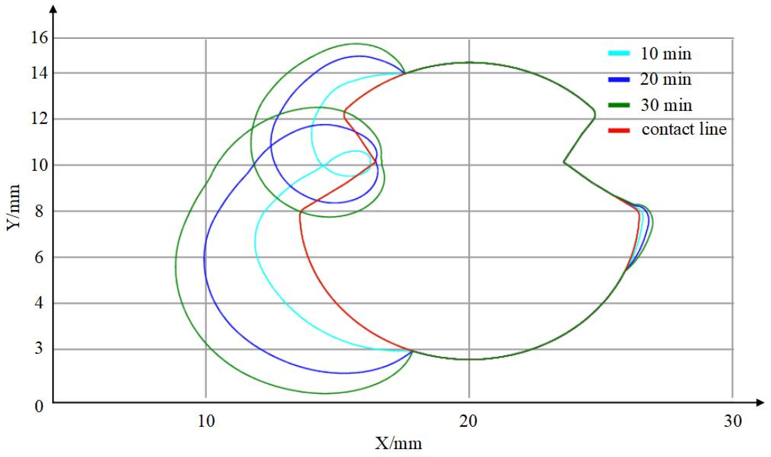
3.2. Contact Line Icing Model Simulation

Based on the transmission conductor icing simulation, a contact line icing simulation was performed, and a case study was selected for verification. The calculation conditions for the case study are as follows: the incoming wind speed v is 15 m/s, ambient temperature is −5 °C, droplet diameter is 20 μm, and the air–liquid water content (LWC) is 0.5 g/m³. This study was divided into three time periods, with data recorded every ten minutes. Figure 7 shows the LWC of Langmuir D distribution droplets around the contact line at a certain moment. Figure 8 shows the distribution contour of the droplet collection coefficient on the contact line surface. Figure 9 presents the icing shapes of the three-dimensional contact line model at different time steps.

Table 3. Maximum ice cover thickness at different time steps.

Time (min)	10	20	30
Maximum ice thickness (mm)	1.775	3.568	4.951

shows the maximum ice cover thickness at different time steps.

As shown in Figure 8, the droplet collection coefficient is highest at the upper and lower sides of the contact line groove. This indicates that under the same icing conditions, the groove area is the most likely region for droplet deposition and is the key area where icing begins first and is most prone to accumulation. Continuous accumulation in this area may ultimately lead to the formation of uneven icing.

As shown in Figure 9 and Table 3, at high wind speeds (15 m/s), the inertial effect of the water droplets becomes more pronounced, allowing the droplets to strike the contact line surface with higher kinetic energy. This not only increases the droplet deposition rate on the windward side, promoting rapid ice layer growth but also causes some droplets to deviate from their original impact trajectory due to the airflow’s bypass effect. These droplets are carried along the contact line by the airflow, gradually expanding the icing range along the upper and lower sides. In addition, under high wind speed conditions, some droplets, after striking the contact line, follow special trajectories due to the airflow’s bypass effect. As the airflow moves around the contact line, it creates specific flow field structures on the leeward side. Some droplets that impact the contact line are carried by the bypass airflow along the surface of the contact line toward the leeward side, where they freeze, resulting in a small amount of ice formation.

Additionally, in some regions of the figures, the boundary of the ice layer appears to extend inside the physical contour of the contact line. This phenomenon is primarily caused by the unique cross-sectional geometry of the contact wire and the mesh discretization used in the CFD modeling. The windward side of the contact line features prominent grooves and concave surfaces. Under high-speed airflow, droplets are influenced by flow deflection and pressure gradients, causing them to follow curved trajectories and impact these recessed areas. Furthermore, in the post-processing stage of the simulation, the ice shape is generated based on the calculated ice thickness at each point on the contact line surface. Since ice growth is defined along the normal local surface, and the surface geometry includes inward curvature, the resulting visualization may, from certain angles, give the impression that the ice extends into the conductor’s body. In reality, these regions are part of the actual windward surface and do not indicate that ice forms within the material itself.

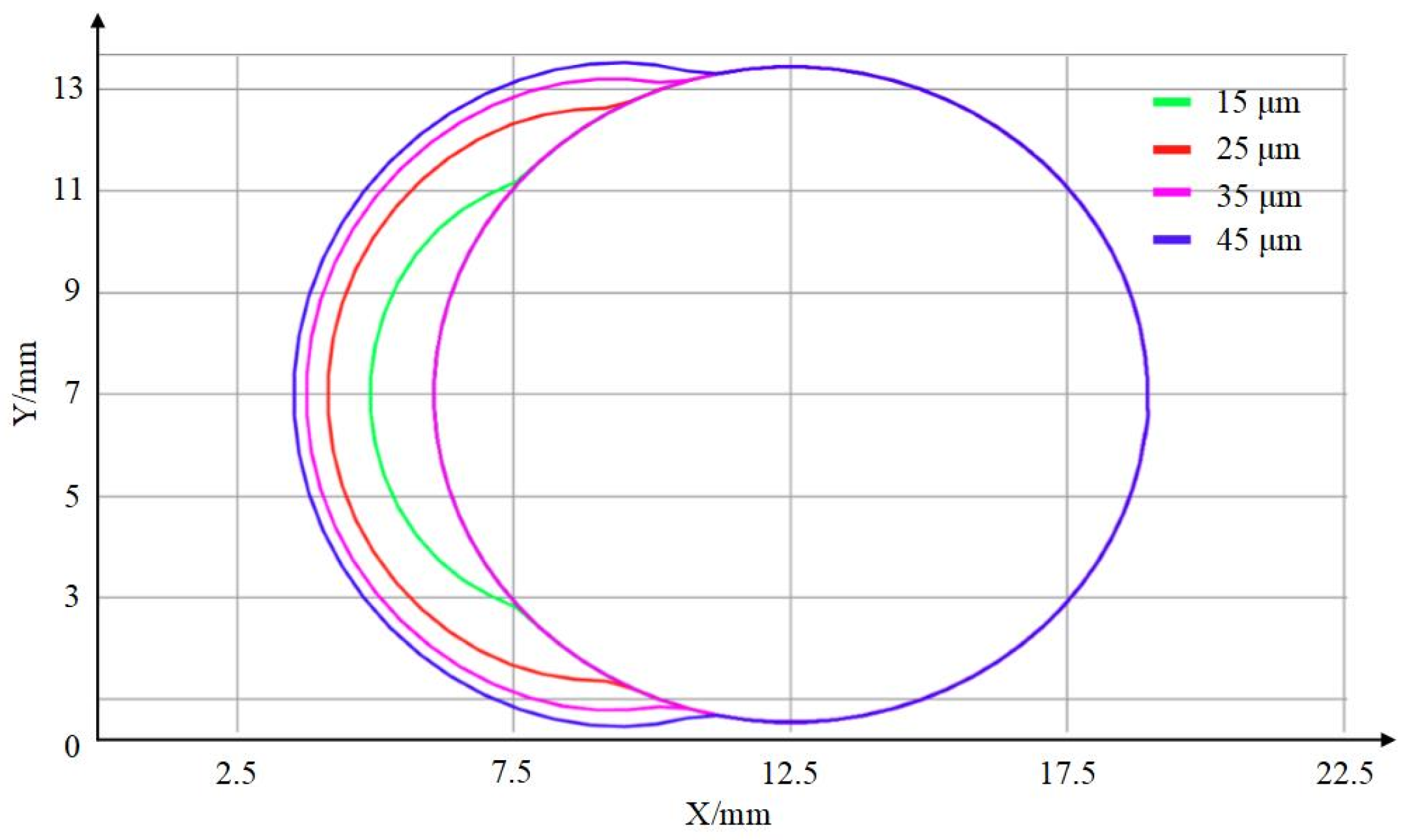
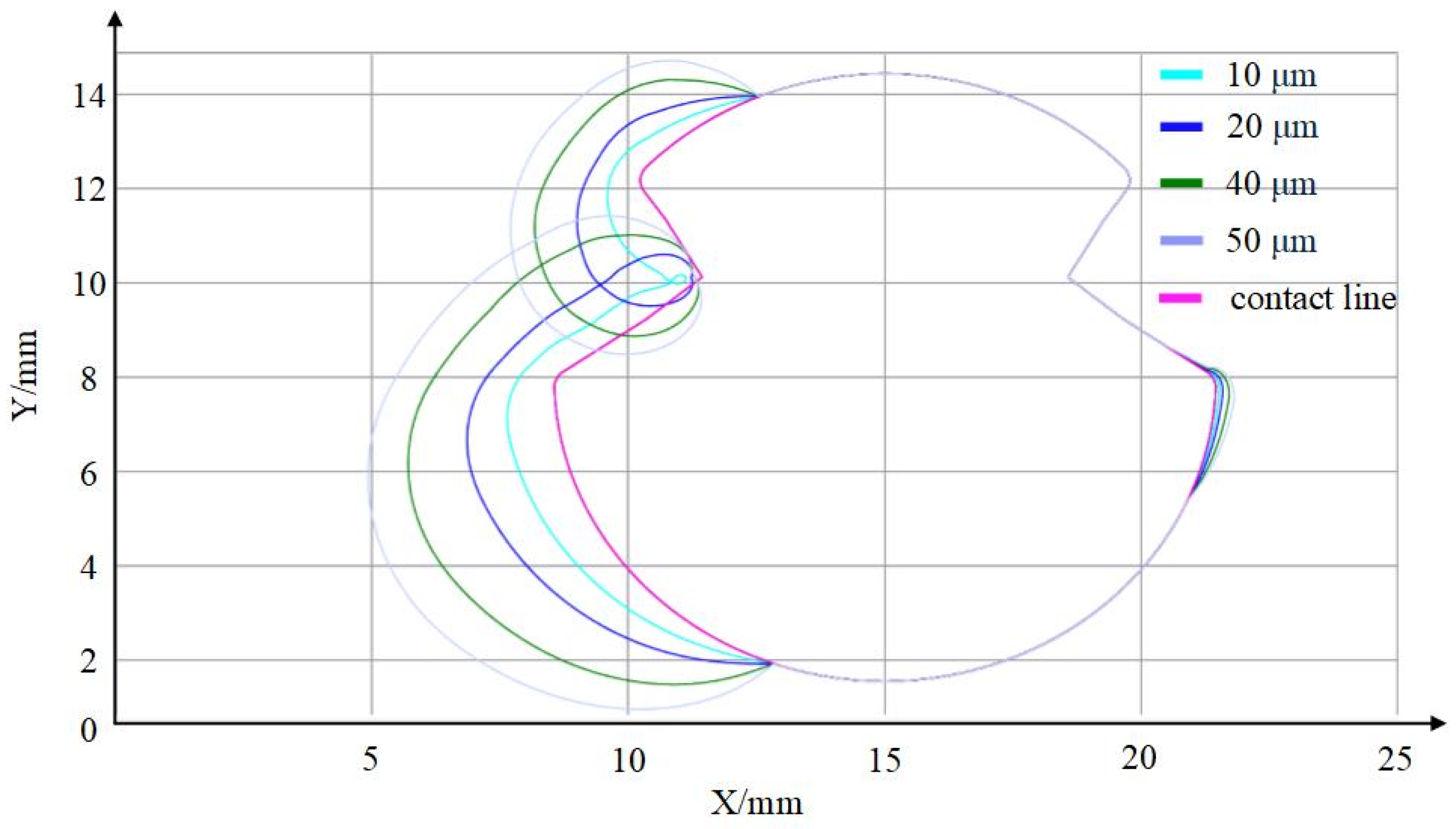
3.3. Analysis of Computational Results for Different Droplet Diameters

Under icing climate conditions, the droplet diameter in the air is typically below 40 μm. With wind speed maintained at 15 m/s, the air–liquid water content is maintained at 0.5 g/m³, the temperature is maintained at −5 °C, and the droplet diameter (MVD) changes to 10 μm, 20 μm, 40 μm, and 50 μm. The resulting icing shapes on the contact line are shown in Figure 10. This analysis explores the effects of different droplet diameters on the icing morphology of the contact line.

Table 4. Maximum ice cover thickness at different droplet diameters.

MVD (μm)	10	20	40	50
Maximum ice thickness (mm)	1.274	1.821	2.359	3.562

shows the maximum ice cover thickness at different droplet diameters.

As shown in Figure 10 and Table 4, the impact of the droplet diameter on the icing morphology of the contact line differs from its effect on the conductor icing morphology. The main reason for this is that the presence of the contact line groove causes the maximum droplet collection coefficient on the contact line surface to be concentrated near the groove rather than evenly distributed across the entire contact line surface. As the droplet diameter increases, the inertial effect of the droplets is enhanced, making them more likely to strike the contact line surface, leading to a significant increase in the accumulated ice mass. However, due to the constraint of the groove structure on the icing area of the contact line, the overall ice-shape profile remains stable, with no significant morphological changes.

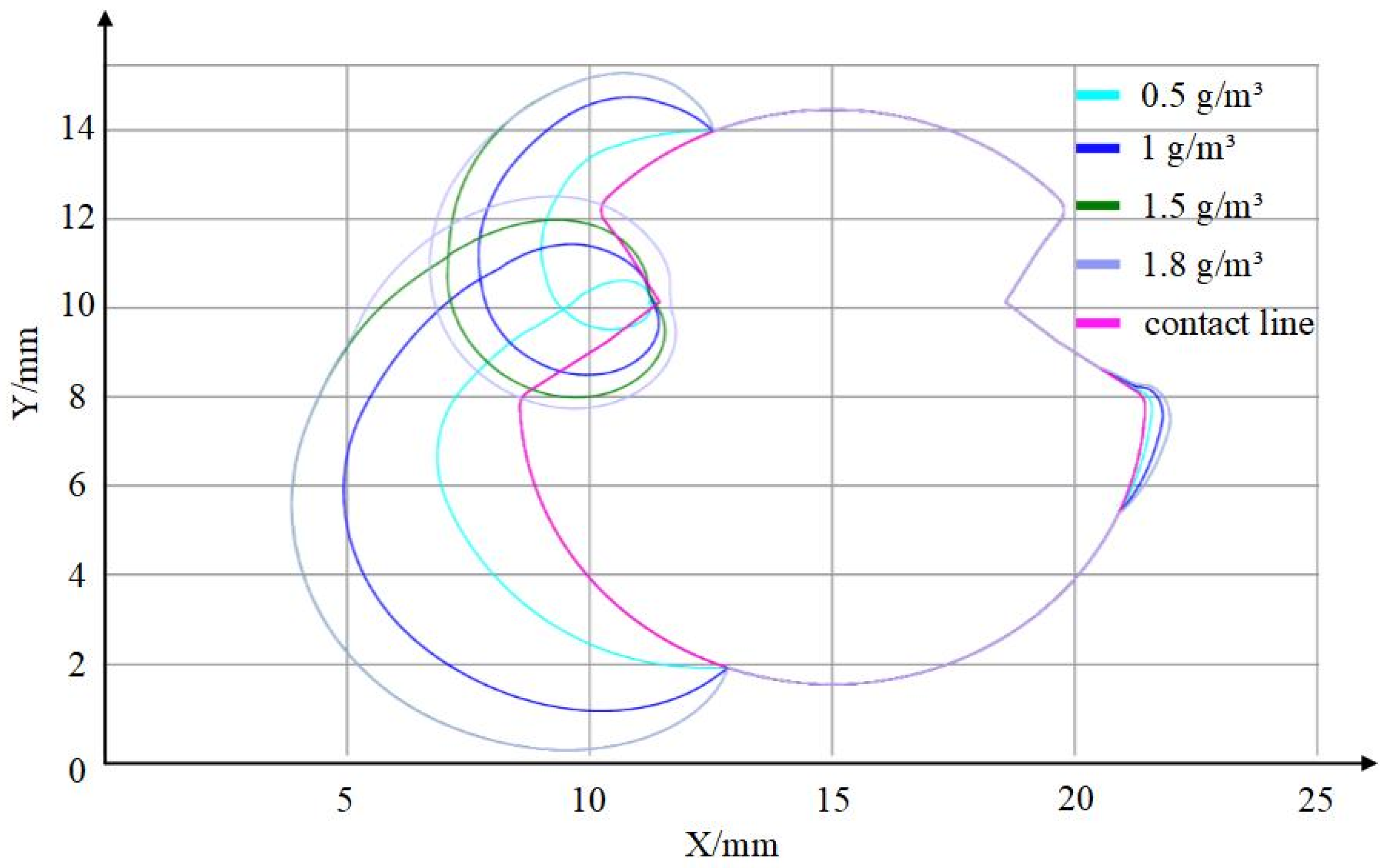
3.4. Analysis of Computational Results for Different Air–Liquid Water Content

The air–liquid water content (LWC) is an important parameter for measuring the amount of suspended liquid water in the air and primarily reflects the concentration of droplets available for freezing. The value of LWC directly determines the amount of water that will freeze on the surface of an object. With the wind speed held constant at 15 m/s, the droplet diameter is maintained at 20 μm, the temperature is maintained at −5 °C, and the air–liquid water content is varied at 0.5 g/m³, 1 g/m³, 1.5 g/m³, and 1.8 g/m³. The resulting icing shapes on the contact line are shown in Figure 11.

Table 5. Maximum ice cover thickness at different air–liquid water contents.

LWC (g/m3)	0.5	1	1.5	1.8
Maximum ice thickness (mm)	1.837	3.556	5.012	5.012

shows the maximum ice cover thickness at different air–liquid water contents.

As shown in Figure 11 and Table 5, the amount of icing on the contact line surface increases with the increase in the air–liquid water content, and the ice thickness also increases accordingly. When the liquid water content in the air increases, the number of water droplets suspended in the air rises, leading to an increase in the number of droplets striking the contact line surface per unit of time, thus resulting in the continuous accumulation of ice. However, the upper and lower extreme positions of the contact line icing remain unchanged. This is because when only the air–liquid water content is changed, the collision characteristics of the water droplets in the air do not change, which does not affect the droplets’ movement path or impact location, so the limited positions of droplet collisions remain unchanged.

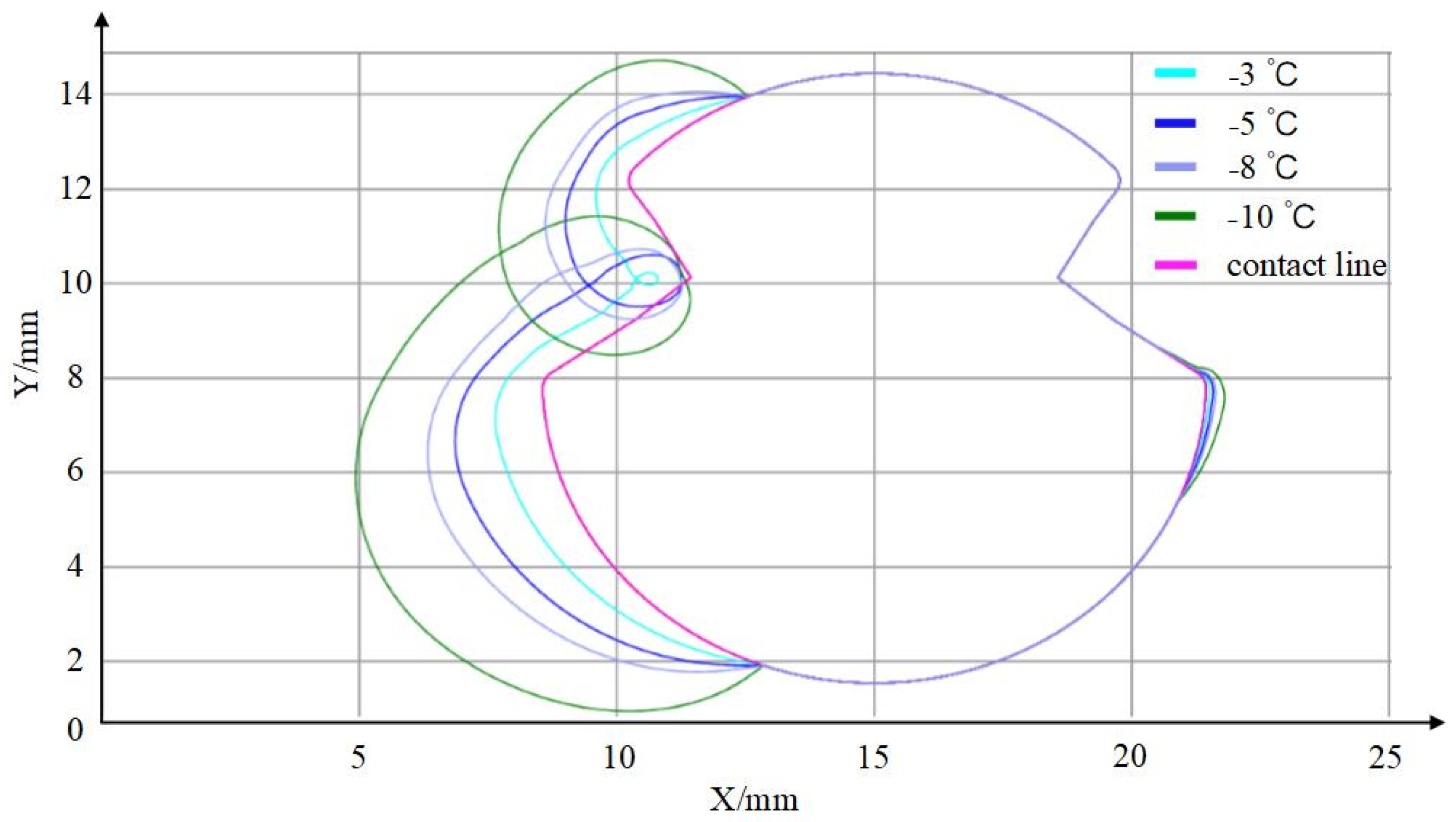
3.5. Analysis of Computational Results at Different Ambient Temperatures

With wind speed maintained at 15 m/s, air–liquid water content is maintained at 0.5 g/m³, the droplet diameter is maintained at 20 μm, and the ambient temperature is varied to −3 °C, −5 °C, −8 °C, and −10 °C. The resulting icing shapes on the contact line at different ambient temperatures are shown in Figure 12.

Table 6. Maximum ice cover thickness at different ambient temperatures.

Temperatures (°C)	−3	−5	−8	−10
Maximum ice thickness (mm)	1.345	1.853	2.184	3.589

shows the maximum ice cover thickness at different ambient temperatures.

As seen in Figure 12 and Table 6, as the ambient temperature decreases, the amount of icing and ice thickness on the contact line surface continuously increases. Temperature primarily affects the thermodynamic process during the contact line icing process. As the temperature drops, convective heat transfer in the air intensifies. When water droplets impact the contact line, they need to absorb more heat to reach the freezing point, which accelerates heat dissipation from the contact line surface, causing the droplets to freeze more quickly and increasing the amount of icing per unit of time. Additionally, under higher temperature conditions, some water droplets remain in a liquid state and do not fully freeze. As the temperature continues to decrease, the number of frozen droplets increases, ultimately leading to a significant increase in ice thickness.

4. Conclusions

This study is based on the CFD three-dimensional numerical simulation method to explore the icing process of electrified railway contact lines under different environmental parameters. The effectiveness of the model is verified by comparing it with traditional transmission conductors. The research not only reveals the influence of factors such as water droplet diameter, air–liquid water content, and ambient temperature on the icing behavior but also investigates the differential icing characteristics brought about by the special cross-section of the contact line. The main conclusions are as follows:

(1)

Compared with traditional circular conductors, due to the obvious tail-groove structure and asymmetric cross-section of the contact line, the water droplet collection coefficient on the windward side shows a locally concentrated distribution, and the icing morphology is more likely to develop asymmetrically up and down. However, due to the symmetrical structure of the conductor, the icing morphology is more uniform and has fuller icing.

(2)

Under different water droplet diameters and air–liquid water contents, although the thickness of the ice layer on the contact line changes significantly, restricted by the groove and edge structures, the expansion of the icing area is limited, and the limited position of the icing area is more stable.

(3)

Under the condition that the wind speed reaches 15 m/s, some water droplets, after the first impact on the surface of the contact line, are carried to its downstream surface by the bypass airflow, slide along the surface curvature, and freeze, forming a small-scale “secondary icing area” on the leeward side of the contact line. This phenomenon is not obvious in the conductor simulation, indicating that the geometric characteristics of the contact line are more sensitive to the disturbed airflow, and the icing area is more complex.

References

1. Wang, J.; Mei, G.; Lu, L. Analysis of the pantograph’s mass distribution affecting the contact quality in high-speed railway. Int. J. Rail Transp. 2022, 11, 529–551. [Google Scholar] [CrossRef]
2. Agüero-Barrantes, P.; Hain, A. Structural performance of porcelain insulators in overhead railway power systems: Experimental evaluations and findings. Infrastructures 2024, 9, 138. [Google Scholar] [CrossRef]
3. Wang, X.; Song, Y.; Lu, B.; Wang, H.; Liu, Z. Assessment of current collection performance of rail pantograph-catenary considering long suspension bridges. IEEE Trans. Instrum. Meas. 2025, 74, 7500714. [Google Scholar] [CrossRef]
4. Song, Y.; Liu, Z.; Gao, S. Current Collection Quality of High-Speed Rail Pantograph-Catenary Considering Geometry Deviation at 400 km/h and Above. IEEE Trans. Veh. Technol. 2024, 73, 14415–14424. [Google Scholar] [CrossRef]
5. Liu, Z.; Song, Y.; Gao, S.; Wang, H. Review of Perspectives on Pantograph-Catenary Interaction Research for High-Speed Railways Operating at 400 km/h and Above. IEEE Trans. Transp. Electrif. 2024, 10, 7236–7257. [Google Scholar] [CrossRef]
6. Makkonen, L.; Lozowski, E.P. Numerical Modeling of Icing on Power Network Equipment. In Atmospheric Icing of Power Networks; Springer: Dordrecht, The Netherlands, 2008; pp. 83–117. [Google Scholar]
7. Xingbo, H.; Xingliang, J. Analysis of critical condition for dry and wet growth icing on insulators. Electr. Power Syst. Res. 2021, 192, 107006. [Google Scholar]
8. Tabakova, S.; Feuillebois, F. On the solidification of a supercooled liquid droplet lying on a surface. J. Colloid Interface Sci. 2004, 272, 225–234. [Google Scholar] [CrossRef]
9. Prodi, F.; Levi, L.; Levizzani, V. Ice accretions on fixed cylinders. Q. J. Roy. Meteorol. Soc. 1986, 112, 1091–1109. [Google Scholar] [CrossRef]
10. Fumoto, K. Experimental Study on the Critical Heat Flux of Ice Accretion Along a Fine Wire Immersed in a Cold Air Flow with Water Spray. Adv. Cold Region Therm. Eng. Sci. 1999, 533, 45–54. [Google Scholar]
11. Lu, L.M.; Popplewell, N.; Shah, H.A. Freezing rain simulations for fixed, unheated conductor samples. Am. Meteorol. Soc. 2000, 39 Pt 2, 2385–2396. [Google Scholar] [CrossRef]
12. Personne, P.; Gayet, J.F. Ice Accretion on Wires and Anti-Icing Induced by Joule Effect. J. Appl. Meteorol. 2010, 27, 101–114. [Google Scholar] [CrossRef]
13. Zhao, C.; Wang, T.; Zhou, G.; Wang, Y.; Feng, Y.; Jiang, C.; Song, Z.; Li, H. Wind tunnel experimental investigation on the performance of the ice-melting system for high-speed train bogies. Transp. Saf. Environ. 2025, 7, tdae022. [Google Scholar] [CrossRef]
14. Wang, H.; Liu, Z.; Hu, G.; Wang, X.; Han, Z. Offline Meta-Reinforcement Learning for Active Pantograph Control in High-Speed Railways. IEEE Trans. Ind. Inform. 2024, 20, 10669–10679. [Google Scholar] [CrossRef]
15. Wang, H.; Liu, Z.; Han, Z. HO2RL: A Novel Hybrid Offline-and-Online Reinforcement Learning Method for Active Pantograph Control. IEEE Trans. Ind. Electron. 2025, 72, 6286–6296. [Google Scholar] [CrossRef]
16. Savadjiev, K.; Farzaneh, M. Modeling of icing and ice shedding on overhead power lines based on statistical analysis of meteorological data. IEEE Trans. Power Deliv. 2004, 19, 715–721. [Google Scholar] [CrossRef]
17. Jiang, X.; Fan, S.; Zhang, Z.; Sun, C.; Shu, L. Simulation and Experimental Investigation of DC Ice-Melting Process on an Iced Conductor. IEEE Trans. Power Deliv. 2010, 25, 919–929. [Google Scholar] [CrossRef]
18. Yang, L.; Hu, Z.; Nian, L.; Hao, Y.; Li, L. Prediction on freezing fraction and collision coefficient in ice accretion model of transmission lines using icing mass growth rate. IET Gener. Transm. Distrib. 2021, 16, 364–375. [Google Scholar] [CrossRef]
19. Xu, F.; Li, D.; Gao, P.; Zang, W.; Duan, Z.; Ou, J. Numerical simulation of two-dimensional transmission line icing and analysis of factors that influence icing. J. Fluids Struct. 2023, 118, 103858. [Google Scholar] [CrossRef]
20. Morris, J.; Robinson, M.; Palacin, R. Use of dynamic analysis to investigate the behaviour of short neutral sections in the overhead line electrification. Infrastructures 2021, 6, 62. [Google Scholar] [CrossRef]
21. Chen, G.; Yang, Y.; Yang, Y.; Li, P. Study on Galloping Oscillation of Iced Catenary System under Cross Winds. Shock Vib. 2017, 2017, 1634292. [Google Scholar] [CrossRef]
22. Sadov, S.Y.; Shivakumar, P.N.; Firsov, D.; Lui, S.H.; Thulasiram, R. Mathematical Model of Ice Melting on Transmission Lines. J. Math. Model. Algorithms 2007, 6, 273–286. [Google Scholar] [CrossRef]
23. Li, Z.; Wu, G.; Huang, G.; Guo, Y.; Zhu, H. Study on Icing Prediction for High-Speed Railway Catenary Oriented to Numerical Model and Deep Learning. IEEE Trans. Transp. Electrif. 2024, 11, 1189–1200. [Google Scholar] [CrossRef]
24. Wang, W.; Zhao, D.; Fan, L.; Jia, Y. Study on Icing Prediction of Power Transmission Lines Based on Ensemble Empirical Mode Decomposition and Feature Selection Optimized Extreme Learning Machine. Energies 2019, 12, 2163. [Google Scholar] [CrossRef]
25. Peter, Z.; Farzaneh, M.; Kiss, L.I. Assessment of the Current Intensity for Preventing Ice Accretion on Overhead Conductors. IEEE Trans. Power Deliv. 2007, 22, 565–574. [Google Scholar] [CrossRef]
26. Cinieri, E.; Fumi, A. Deicing of The Contact Lines of the High-Speed Electric Railways: Deicing Configurations. Experimental Test Results. IEEE Trans. Power Deliv. 2014, 29, 2580–2587. [Google Scholar] [CrossRef]
27. Snaiki, R.; Jamali, A.; Rahem, A.; Shabani, M.; Barjenbruch, B.L. A Metaheuristic-Optimization-Based Neural Network for Icing Prediction on Transmission Lines. Cold Reg. Sci. Technol. 2024, 224, 104249. [Google Scholar] [CrossRef]
28. Meng, X.; Tian, L.; Liu, J.; Jin, Q. Failure Prediction of Overhead Transmission Lines Incorporating Time Series Prediction Model for Wind-Ice Loads. Reliab. Eng. Syst. Saf. 2025, 259, 110927. [Google Scholar] [CrossRef]
29. Wang, F.; Lin, H.; Ma, Z. Transmission Line Icing Prediction Based on Dynamic Time Warping and Conductor Operating Parameters. Energies 2024, 17, 945. [Google Scholar] [CrossRef]
30. Wang, G.; Shen, J.; Jin, M.; Huang, S.; Li, Z.; Guo, X. Prediction Model for Transmission Line Icing Based on Data Assimilation and Model Integration. Front. Environ. Sci. 2024, 12, 1403426. [Google Scholar] [CrossRef]
31. Wang, H.; Liu, Z.; Song, Y.; Jiang, J. Aerodynamic parameters simulation and wind-induced vibration responses of contact wire of high-speed railway. J. Vib. Shock 2015, 34, 6–12. [Google Scholar]
32. Makkonen, L. Models for the Growth of Rime, Glaze, Icicles and Wet Snow on Structures. Philos. Trans. Math. Phys. Eng. Sci. 2000, 358, 2913–2939. [Google Scholar] [CrossRef]
33. Fu, P. Modelling and Simulation of the Ice Accretion Process on Fixed or Rotating Cylindrical Objects by the Boundary Element Method; Universite du Quebec a Chicoutimi: Chicoutimi, QC, Canada, 2004; pp. 62–66. [Google Scholar]
34. Song, Y.; Liu, Z.; Wang, H.; Lu, X.; Zhang, J. Nonlinear analysis of wind-induced vibration of high-speed railway catenary and its influence on pantograph-catenary interaction. Veh. Syst. Dyn. 2016, 54, 723–747. [Google Scholar] [CrossRef]
35. Gao, P.; Zang, W.; Li, D. Numerical simulation and analysis of influencing factors of icing on transmission lines. J. Vib. Shock. 2023, 42, 77–85. [Google Scholar]
Figure 1. CuAg0.1AC120-type contact line cross-section.
Infrastructures 10 00121 g001
Figure 2. Contact line mesh diagram: (a) flow region mesh; (b) local grid zoom.
Infrastructures 10 00121 g002
Figure 3. Flow region analysis of contact line: (a) surface pressure contour map; (b) surface velocity contour map.
Infrastructures 10 00121 g003
Figure 4. Mesh-independent verification.
Infrastructures 10 00121 g004
Figure 5. Schematic diagram of droplet collision.
Infrastructures 10 00121 g005
Figure 6. Icing patterns of transmission conductors under different droplet diameters.
Infrastructures 10 00121 g006
Figure 7. LWC of Langmuir D distribution droplets around the contact line.
Infrastructures 10 00121 g007
Figure 8. Droplet collection coefficient distribution contour on the contact line surface.
Infrastructures 10 00121 g008
Figure 9. The icing shape of the contact line at different time steps.
Infrastructures 10 00121 g009
Figure 10. Icing morphology for different droplet diameters.
Infrastructures 10 00121 g010
Figure 11. Icing morphology for different air–liquid water contents.
Infrastructures 10 00121 g011
Figure 12. Icing morphology at different ambient temperatures.
Infrastructures 10 00121 g012