Abstract
Structural damage detection is essential for civil infrastructure safety. The challenges in noise sensitivity, multi-scale feature extraction, and handling bidirectional temporal dependencies are often encountered by traditional methods such as vibration analysis and computer vision. Although potential solutions are offered by recent deep-learning advancements, limitations are frequently imposed by low interpretability and the incapability to adaptively prioritize crucial features within complex time-series data. To address these, a novel hybrid deep-learning framework is proposed. It is integrated with multi-scale convolutional neural networks (CNNs), bidirectional long short-term memory (BiLSTM) networks, and attention mechanisms. Localized time-frequency features are captured from vibration signals by the CNN using multi-scale kernels. Bidirectional temporal dependencies are skillfully captured by the BiLSTM. The interpretability is improved by the attention mechanism through dynamic feature weighting. Experiments on a simulated steel frame demonstrate that detection accuracy and robustness can be enhanced by this framework. This work promotes structural health monitoring, providing a practical tool for engineering applications.
1. Introduction
During the long-term service of engineering structures, under the influence of natural loads (such as wind, earthquakes, temperature changes, etc.) and human-induced loads (such as vehicle loads, construction loads, etc.), damage is prone to occur. Changes in the dynamic characteristics of the structure, such as stiffness, frequency, or the vibration mode, can be caused by these damages. In severe cases, the collapse of the structure may be caused, resulting in huge economic losses and social impacts [1]. Therefore, the timely and effective identification and assessment of structural damage is of great significance for ensuring engineering safety.
Physical signal detection technologies, such as the ultrasonic method, the computer vision method, and the vibration signal method, are mainly encompassed by traditional structural damage detection methods. In the ultrasonic method, damage is identified by detecting the ultrasonic signals inside the structure. The detailed information about internal damage can be provided by this method; it is beneficial for realizing real-time monitoring [2]. However, the penetration depth is limited by the ultrasonic method. The polishing of the structural surface is required during detection, and the equipment cost is relatively high. For the computer vision method, the structural damage is detected using the image data captured by a camera [3,4]. Advantages such as low cost and simple operation are included in this method [5]. However, it is difficult to identify the internal damage with this method. The high requirements are imposed on environmental conditions and the line of sight, and a large amount of data support is required. In the vibration signal method, the damage is identified by analyzing the vibration response signals of the structure. The structural damage can be effectively identified and located by this method [6,7]. However, this method is sensitive to noise, and the convergence speed is slow [8,9]. In the study of [10], a noise robustness framework based on a multi-channel convolutional autoencoder and empirical mode decomposition is proposed. By screening highly correlated eigenmode functions and combining wavelet transform, the damage identification ability of vibration signals in noisy environments is significantly improved, providing a new idea for real-time monitoring under complex working conditions. In practical applications, problems such as high computational cost, great influence by the sensor location, and large data storage requirements exist.
In recent years, with the rapid development of artificial intelligence, the structural damage identification methods based on machine learning are widely applied. The remarkable results in structural damage detection are achieved by traditional machine learning algorithms such as the support vector machine (SVM) [11,12], decision tree (DT) [13], and residual network (ResNet) [14]. In the study of [15], a multi-channel data fusion method based on multiple deep belief network is proposed. In the study of [16], the fault identification of rotating machinery is realized through signal visualization. However, the large-scale and high-dimensional data are usually found difficult to be handled by these methods. Recently, the data-driven methods using a convolutional neural network (CNN) are developed for structural health monitoring (SHM). These methods are endowed with powerful nonlinear fitting and feature extraction capabilities [17]. As a deep-learning model, a powerful feature-extraction ability is possessed by the CNN. The features are automatically extracted from data by it, and the handling of complex and large-scale data is enabled. In the study of [18], by fusing the horizontal and vertical vibration signals from different positions, a deep CNN is trained to evaluate the damage status of planetary gears. In the study of [19], a method for searching the optimal CNN structure that can predict the structural response to evaluate the long-term safety of the structure is proposed. However, the multi-scale feature-extraction ability is lacked by the traditional CNN model. Building on this, a hybrid CNN-SVM framework [20] is proposed that not only leverages deep feature extraction from the CNN but also incorporates the SVM’s strong classification capability, demonstrating superior performance on limited datasets. Directly capturing the multi-scale features in the time series is made difficult for it, resulting in the model’s performance being limited when dealing with complex time-series data [21]. In order to better handle the complex dependencies in time-series data, the long short-term memory network (LSTM) is introduced into the field of SHM. In the study of [22], a method combining a multi-scale ResNet and an LSTM model is proposed to realize the condition monitoring of the gearbox. However, the unidirectional dependence of the time series, namely, the flow of information from the past to the future, is mainly focused on by the LSTM model. To further improve the model’s ability to process time-series data, the bidirectional long short-term memory network (BiLSTM) is proposed. The past and future information of time-series data is simultaneously captured by the BiLSTM model through bidirectional sequence processing, enabling a more comprehensive feature representation to be provided [23]. This fusion of bidirectional information endows the BiLSTM model with stronger expressive capabilities when applied to time-series data analysis. In structural damage detection, the bidirectional dependencies of vibration signals are effectively handled by the BiLSTM, and the accuracy of damage identification is improved.
Although excellent performances are achieved by the CNN and BiLSTM in feature extraction and time-series data processing, the “black box” problem is long existent in deep-learning models. That is, the decision-making process of the model lacks transparency, and it is difficult to explain why specific predictions are made by the model [24]. The application of the model in practical engineering, especially in the field of SHM where high reliability and interpretability are required, is limited by this “black box” characteristic. In order to solve this problem, the attention mechanism is widely used to enhance the transparency of deep-learning models. Which features play a key role in the final decision- making is clearly shown by the attention mechanism through dynamic weight assignments [25,26]. The damage features can not only be better identified and located by the model with the help of the attention mechanism, but also the interpretability of the model can be improved by it. By visualizing the attention weights, the feature areas that the model focuses on when making decisions can be intuitively understood by researchers, thus enhancing the understanding of the model’s decision-making process. In the study of [27], an interpretable framework based on vision Transformer (ViT) is proposed to analyze the model decision logic through the patch attention mechanism and reveal the damage characteristics of the model’s concern through the visualization of key areas, which significantly improves the reliability of diagnosis results. The feature weights of the model combined with the attention mechanism can be adaptively adjusted by introducing the attention mechanism, and the model’s feature-extraction ability can be further improved. Different weights are enabled to be assigned to different features by the attention mechanism, allowing the model to pay more attention to key features, thus improving the model’s performance.
Based on the above background, a structural damage detection model combining the CNN, BiLSTM, and the attention mechanism (CNN-BiLSTM-Attention model) is proposed. The following are the main contributions of this paper.
- (1)
- A structural damage detection model combining CNN, BiLSTM, and the attention mechanism is proposed in this paper. Local time-frequency features are extracted by the CNN in this model, long-term dependencies in the time series are captured by the BiLSTM, and the ability to identify key damage features is enhanced by the attention mechanism. The strengths of each component are effectively combined by this integrated approach to improve damage detection accuracy.
- (2)
- To improve the model’s feature-capturing ability and enhance its interpretability, the attention layer is introduced. The feature domains emphasized by the model during the decision-making process can be intuitively grasped by researchers through the visualization of attention weights. Thus, the understanding of the decision-making mechanism is deepened.
- (3)
- The Focal Loss function is introduced to address the problems of sample imbalance and misclassification of confusing samples in structural damage detection. Based on the Cross-Entropy Loss, different weights are assigned to samples of various categories. The defined weight and adjustment factors, with default values and adaptable settings for specific working condition types, offer a practical mechanism for fine-tuning the model. Thus, the overall classification accuracy in structural damage detection is improved.
The structural arrangement of this paper is as follows: Section 2 details the structure and principle of the CNN-BiLSTM-Attention model. Section 3 describes the experimental setup, experimental results, and their analysis. Section 4 summarizes the main contributions of this paper and prospects future research directions.
2. Methodology
A structural health monitoring (SHM) evaluation model was established by combining CNN, BiLSTM and the attention mechanism. The structure of the CNN-BiLSTM-At SHM model is shown in Figure 1. For the time-series data, the local time-frequency features of the data within T time steps were learned by the CNN network. The long-term dependencies in the time series were captured through the BiLSTM. The importance of the features of the time-series data from each sensor was evaluated by the attention mechanism. This means that the importance of features at different positions in the SHM evaluation can be evaluated by the attention mechanism.
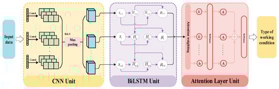
Figure 1.
The structural diagram of the CNN-BiLSTM-At SHM model.
2.1. CNN Unit
The convolutional neural network (CNN) [19] was applied to extract features from the acceleration response signals of the steel frame structure. The local time-frequency features of the structural vibration signals were effectively captured by the CNN through the one-dimensional convolutional layer (nn.Conv1d). Taking the acceleration response signal data as the input, the formula for the convolutional operation is calculated as follows:
where represents the i-th feature of the output value of the n-th layer; represents the weight matrix of the i-th convolutional kernel of the n-th layer; the ∗ operator represents the convolutional operation; is the output of the (i − 1)-th layer; represents the bias term; and the function represents the activation function ReLU of the output.
Then, the feature vector was fed into the global average pooling layer. The average value was calculated for the data of each output channel, the robustness of the model was increased by it. At the same time, the number of parameters was reduced, overfitting of the model was prevented, and the convergence speed of the model was accelerated.
2.2. BiLSTM Unit
The BiLSTM network is a variant of the LSTM network. It is composed of a forward LSTM network and a backward LSTM network combined together. The LSTM network [28,29] is an improvement of the recurrent neural network (RNN). The LSTM network is a special type of RNN. It is designed to solve the problem of gradient vanishing or explosion in traditional RNN when dealing with long sequence data. The LSTM introduced three gating mechanisms—the input gate, the forget gate, and the output gate—to regulate the flow of information, thus enabling the capture of long-term dependencies. The LSTM unit structure is shown in Figure 2. The LSTM unit calculation process is as follows:
where is the t time memory unit, is the temporary memory unit, represents the multiplication of elements by elements, represents the addition of elements by elements, is the weight matrix corresponding to each module, is the bias term, is the sigmoid activation function, and tanh is the hyperbolic tangent activation function.
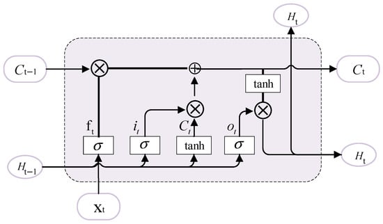
Figure 2.
The structural diagram of the LSTM network.
In order to further enhance the model’s understanding of the dynamic characteristics of sequential data, a BiLSTM [23] network was introduced in this study. The BiLSTM is capable of processing the feature data from the CNN and capturing the long-term dependencies of the signals in the time dimension. Different from the traditional LSTM, the sequential data were processed in both the forward and backward directions simultaneously by the BiLSTM, and a more comprehensive representation of the sequential features was provided. The model is enabled to more accurately identify the damage features of the structure at different time points. Thus, the accuracy and reliability of damage identification were improved. The structural diagram of the BiLSTM network is shown in the following Figure 3.
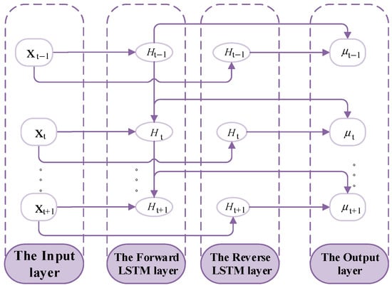
Figure 3.
The structural diagram of the BiLSTM network.
The calculation process of BiLSTM is as follows:
where , , are, respectively, the outputs of the forward LSTM layer state, the backward LSTM layer state, and the output layer state at t time; is the vector input at t time; is the LSTM unit function; is the ReLU function; and is the weight vector.
The association relationships of the forward historical features of the fault were extracted sequentially from the front to the back according to the development direction of the time series by the forward LSTM layer. The association relationships of the historical features of the fault were traced and tracked from the back to the front in the reverse direction of the time series by the backward LSTM layer. The time-series features of the data were obtained by the fusion of these two types of features.
2.3. Attention Layer Unit
The attention mechanism was integrated into the CNN and BiLSTM to enhance the model’s ability to identify key damage features. The model was enabled to adaptively focus on the sequential regions that are most crucial for damage identification by the introduction of attention weighting [24,25]. The output of the BiLSTM layer was weighted by the attention layer with the learned weights, and the contribution degrees of different sequential regions to the final damage identification result were reflected by these weights. In this way, the damage position can be more accurately located, and the severity of the damage can be evaluated by the model. The interpretability of the model was enhanced, and the performance of the classification task was improved.
The working process was divided into three steps. First, the similarity and correlation calculations were carried out between the query and each key to obtain the weight coefficients. Then, the Softmax function was used to standardize and normalize the above weight coefficients. Finally, the weights were weighted and summed with the corresponding values. The main internal calculation formulas are as follows.
where u and W represent the weight, b represents the bias, H represents the output of the BiLSTM network, and represents the different weight coefficients of each output feature.
2.4. Loss Function Construction
For the field of structural damage detection, certain categories of conditions are less likely to be accurately categorized than others, which are called confusing samples for classification [30,31]. However, the sample imbalance caused by the lack of samples in these condition categories is such that, if these confusing samples are not handled, the classification accuracy of the model will be greatly reduced [26]. Therefore, the Focal Loss function was introduced, the different weights to the samples of different categories were given on the basis of the Cross-Entropy Loss, and its formula is as follows.
where is the value of the loss function. , are the true and predicted values of the k-th sample, respectively. is the weight factor, and is the adjustment factor. When the corresponding sample is the sample of the working condition type A for which the weight needs to be increased, the adjustment factor is set to 10. Otherwise, the adjustment factor is set to 1. The problems of similar samples and class imbalance can be better handled by the model by using the Focal Loss. The attention of the model to the samples that are prone to confusion can be increased, and, thus, better classification performance can be achieved.
The local feature extraction ability of the input signals was enhanced by the model through the employment of CNN units. Then, the outputs from the CNNs were processed by a BiLSTM network. The time- dependence of the fault signals was captured via an attention layer so that the focus of the model on the features of the critical points in time can be augmented; thereby the accuracy of fault diagnosis can be improved.
3. Experimental Validation
3.1. Experimental Setup
In this experiment, the input features are obtained through the simulation of a scaled-down model of a 4-story steel frame with two spans in one direction and one span in the other direction, as shown in Figure 4. The simulation is carried out by using the finite element analysis software SAP2000. The height of each floor of the model is 225 mm. The materials of the beams, columns, and diagonal braces are all carbon structural steel Q235. The sectional dimensions and properties are shown in Table 1.
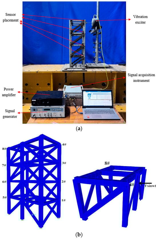
Figure 4.
Schematic diagram of test configuration and excitation setting of steel frame structure: (a) Schematic diagram of steel structure frame and test equipment. (b) Schematic diagram of each level brace number and excitation input direction.

Table 1.
Characteristics of structural members.
Each beam-column joint is welded, so the frame elements are used to simulate the beams and columns of the steel frame. Each end of the diagonal brace is connected to the column gusset plate with one M8 bolt, so the truss elements are used to simulate the diagonal braces. The direction indicated by the arrow in Figure 4b is the input direction of the sinusoidal excitation. Points 1# to 8# are the acceleration output points, with the unit of m/s2, and the direction is the same as that of the external excitation. The sampling frequency is set at 100 Hz, and the sampling duration is set at 5 s. The diagonal braces with notches are taken as the damaged components, and the designed damaged components are shown in Figure 5. The support area of the type 1 diagonal braces is reduced by 10%, and the support area of the type 2 diagonal braces is reduced by 20%. There are six diagonal braces for both type 1 and type 2. The damage of the structure is simulated by replacing the diagonal braces at different positions and with different degrees of damage. The specific damage working conditions are shown in Table 2.
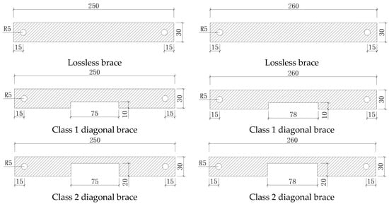
Figure 5.
The design of damaged component.
Table 2.
Units for magnetic properties.
In order to improve the accuracy of the SHM evaluation, the original data obtained from the simulation are standardized using the Z-Score method. In this way, the influence of the units of data with different magnitudes is eliminated, and the comparability among the data is ensured. The calculation formula is as follows:
where is the feature data standardized through the Z-Score method. is the average value of the input original features. is the input original feature quantity. is the standard deviation of the input original features.
The deep learning framework used in the experiment is PyTorch. PyCharm2020.1.3 x64 is adopted as the compilation environment, and the version of Python is 3.9. The entire experimental environment is built based on the PyTorch version 2.3.0 and the CUDA version 13.2. The input data are the acceleration response signal segments of the acceleration output points from 1# to 8# under four kinds of stress conditions, and the length of each acceleration segment is one. In total, 26,000 samples are included in the dataset, and the ratio of the test set to the training set is 1:4. Specifically, there are 5200 samples in the test set, and 20,800 samples in the training set. The learning rate is set at 0.001, the batch size is 256, and the maximum number of training epochs is 100.
3.2. Model Performance Comparison
In order to comprehensively evaluate the performance of the CNN-BiLSTM-At model proposed in this paper, it is compared with models such as the BiLSTM-At, LSTM-At, CNN-At, LSTM, and CNN on the same test set. The CNN-BiLSTM-At model is composed of two convolutional layers, two BiLSTM layers, and an attention layer. A 3 × 3 max pooling layer is connected after each convolutional layer, and each BiLSTM layer contains 128 hidden units. The LSTM layer of the LSTM-At model also contains 128 hidden units. As for the parameters of the remaining models that are the same as those of the model proposed in this paper, these parameters are kept consistent with the corresponding parameters of this model. The performances of different models are shown in Table 3, Table 4 and Table 5.
Table 3.
Accuracy of different models.
Table 4.
Recall of different models.
Table 5.
F1 score of different models.
As seen in Table 3, the CNN-BiLSTM-At model has superiority over other models. Under different stress conditions, a high accuracy can be maintained by the CNN-BiLSTM-At model. Integrating these four stress scenarios, an overall accuracy as high as 96.40% is achieved by it, far exceeding that of other comparative models. It is indicated that signal features can be more effectively captured by the CNN-BiLSTM-At model, and significantly higher accuracy and stability in structural damage identification are possessed by this model. The accuracy and loss of the CNN-BiLSTM-At model on the training set are shown in Figure 6, and the evaluation results of the CNN-BiLSTM-At model on the test set are shown in Figure 7.
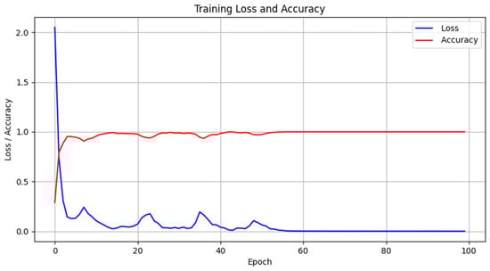
Figure 6.
The training process curve.
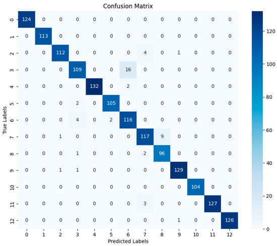
Figure 7.
The CNN-BiLSTM-At model confusion matrix.
3.3. Model Interpretability Analysis
In this study, the method of visualizing attention layer weights is adopted to validate the interpretability of the CNN-BiLSTM-At model and reveals how it identifies damage features of the four-layer steel frame structure. By this method, the feature regions focused on by the model during damage identification can be presented intuitively. Based on the attention weights of sensor signals at different positions and combined with specific damage locations of working conditions, the rationality of the model’s prediction can be verified. Take working conditions 7, 8, 11, and 12 as examples. Their damage locations are complex (7 and 8 are similar, 11 and 12 are similar). The model’s interpretability is analyzed in-depth by outputting the attention weights of corresponding samples. The feature attention distribution maps of these samples are shown in Figure 8 and Figure 9.
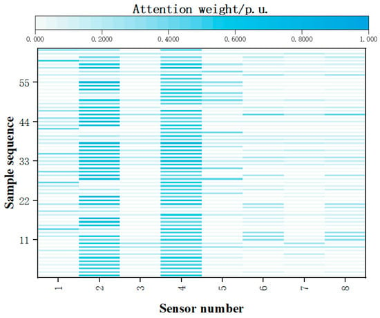
Figure 8.
The characteristic attention distribution diagram of working conditions 7 and 8.
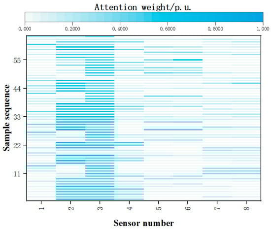
Figure 9.
The characteristic attention distribution diagram of working conditions 11 and 12.
As can be seen from Figure 8 and Figure 9, the main damage locations of the corresponding working conditions can be accurately captured by the model proposed in this paper. Specifically, the damage locations of working conditions 7 and 8 are at the 2nd and 4th sensor positions. From the attention distribution, it can be noticed that, under such working conditions, the attention distribution of the model is also concentrated on the features of the signals from these two sensors. The damage locations of working conditions 11 and 12 are at the 2nd and 3rd detection points. Similarly, the attention distribution of the model is also concentrated on the features of the 2nd and 3rd detection points.
3.4. Accelerated Fragment Length Experiment
In order to explore and evaluate the specific impacts of different lengths of acceleration segments on the performance of the CNN-BiLSTM-At model, the original acceleration response signal data are enhanced by the sliding window technique. Acceleration segments of different lengths are generated to simulate the dynamic behavior of the structure within different time periods. Not only is the diversity of the model training data increased by this approach, but also the sensitivity of the model to the length of time-series information is explored. The evaluation results are shown in Table 6.
Table 6.
Performances of different lengths of acceleration segments.
As shown in Table 6, a significant improvement in the model’s accuracy is presented as the length of the input acceleration segments increases. Specifically, when the segment length is increased from 5 to 25, the model’s accuracy is steadily improved from 96.71% to 99.78%. This result indicates that more abundant time-series information can be provided by longer segments, and the dynamic characteristics and potential damage patterns of the structure can be more comprehensively captured by the model.
When the length of the acceleration segment reached 25, a detailed analysis is carried out for different loading conditions, including different force magnitudes (F = 50 N and F = 100 N) and different frequencies (ω = 50 Hz and ω = 100 Hz). In each case, excellent performance is demonstrated by the CNN-BiLSTM-At model. Whether under low-frequency or high-frequency excitations, or under the action of forces of different magnitudes, the damage states of the structure could be accurately identified by the model. The evaluation results are shown in Table 7.
Table 7.
Performances of different loading conditions.
It can be seen from Table 7 and Figure 10 that, when the acceleration segments are long enough, the damage conditions of the structure can be accurately identified by the model.
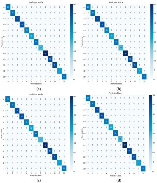
Figure 10.
The mixed matrices under different forces: (a) F = 50 N, w = 50 Hz. (b) F = 50 N, w = 100 Hz. (c) F = 100 N, w = 50 Hz. (d) F = 100 N, w = 100 Hz.
3.5. Noise Experiment
In order to explore and evaluate the specific impact of different noise environments on the performance of the CNN-BiLSTM-At model, the Gaussian noise of 30 dB, 20 dB, and 10 dB are added to the test set, respectively, under mixed four forces to test the accuracy of each model. The results are shown in Table 8.
Table 8.
Performances of different models under different noise conditions.
As shown in Table 8, 91.54% accuracy is maintained by CNN-BiLSTM-At at 10 dB noise, with other models exhibiting significant declines.
3.6. Reasonableness Verification of Weight Factor
We determined the optimal value of weighting factor in Focal Loss to solve the problem of sample imbalance. The experimental results are shown in Table 9.
Table 9.
Performances under different weighting factors.
When the value of the weight factor is within a certain range, the model can be optimized effectively. If the value is too large or too small, it may have a certain impact on the training process. Therefore, we should pay attention to the value of weight factor in the training process.
3.7. Model Efficiency Experiment
In order to evaluate the computational efficiency of the model, this study conducted experiments from two dimensions: training time and evaluation time. The experimental environment is NVIDIA RTX 3090 GPU, Intel i7-12900K CPU, and 32 GB RAM. The experimental results are shown in Table 10.
Table 10.
Efficiency of different models.
It is shown that, although a slightly longer training time is required for CNN-BiLSTM-At, a balance between model performance and computational efficiency is achieved through high evaluation-phase efficiency, combining complex feature extraction capabilities with practical deployment advantages.
3.8. Five-Fold Cross-Validation Experiment
To verify the generalization ability of the model, a 5-fold cross-validation strategy is adopted. The experimental results are shown in Table 11.
Table 11.
Results of 5-fold cross-validation.
It is shown that the model is insensitive to data partitioning, and good robustness is demonstrated, which is attributed to the effective combination of Focal Loss function and attention mechanism.
4. Conclusions
In this paper, a structural damage detection model combining the CNN, BiLSTM, and attention mechanism is proposed, and its effectiveness in the damage identification of steel frame structures is verified through experiments.
It is shown by the experimental results that the comprehensive accuracy in the damage detection of four-layer steel frame structures is reached up to 96.40% by the CNN-BiLSTM-Attention model. When the input sequence length is 25, the accuracy is further increased to 99.78%, which is significantly better than that of traditional models. The short-term, medium-term, and long-term characteristics of vibration signals are captured by convolutional kernels of different sizes, solving the limitations of traditional models in multi-scale feature extraction. The forward and backward time-series data are processed simultaneously, and the bidirectional dependencies in vibration signals are fully exploited, improving the accuracy of damage localization. Through the visual analysis of attention weights, the sensor signals corresponding to the damage locations could be clearly focused on by the model, verifying the physical rationality of the model’s decision- making. In addition, the strong robustness is demonstrated by the model under changes in input sequence length, enabling it to adapt to scenarios with incomplete or interfered data in practical engineering.
However, the reflection of the importance of features by the attention weights is the result of the spontaneous training of the model. In future research, physical information should be combined to guide the model training, and the interpretability of the model should be further improved.
Author Contributions
S.W.: conceptualization; formal analysis; software; writing; acquisition. J.L.: data curation; resources; supervision; validation; investigation. All authors have read and agreed to the published version of the manuscript.
Funding
This work was supported by grants from the Fujian Provincial Natural Science Foundation of China (No. 2022J01970), the Natural Science Foundation of Fujian Province (No. 2024J1423), and the Special Fund for Scientific and Technological Innovation of Fujian Agriculture and Forestry University (No. KFB24050A).
Data Availability Statement
Data will be available upon request.
Conflicts of Interest
The authors declare no conflicts of interest.
References
- Wang, D.-H.; Liao, W.-H. Wireless transmission for health monitoring of large structures. IEEE Trans. Instrum. Meas. 2006, 55, 972–981. [Google Scholar] [CrossRef]
- Wang, Z.; Huang, S.; Wang, S.; Zhuang, S.; Wang, Q.; Zhao, W. Compressed Sensing Method for Health Monitoring of Pipelines Based on Guided Wave Inspection. IEEE Trans. Instrum. Meas. 2020, 69, 4722–4731. [Google Scholar] [CrossRef]
- Zhou, Y.; Li, M.; Shi, Y.; Di, S.; Shi, X. Damage Identification Method of Tied-Arch Bridges Based on Equivalent Thrust-Influenced Line. Struct. Control Health Monit. 2024, 2024, 6896975. [Google Scholar] [CrossRef]
- Zhou, Y.; Shi, Y.; Di, S.; Lu, L.; Sun, W. Cable-stayed bridge model updating using a novel approach for deflection influence line identification: Theoretical basis and field validation. Int. J. Struct. Stab. Dyn. 2025, 2401669. [Google Scholar] [CrossRef]
- Pan, Y.; Ma, Y.; Dong, Y.; Gu, Z.; Wang, D. A Vision-Based Monitoring Method for the Looseness of High-Strength Bolt. IEEE Trans. Instrum. Meas. 2021, 70, 5013914. [Google Scholar] [CrossRef]
- Yan, R.; Gao, R.X. Hilbert–Huang Transform-Based Vibration Signal Analysis for Machine Health Monitoring. IEEE Trans. Instrum. Meas. 2006, 55, 2320–2329. [Google Scholar] [CrossRef]
- Wang, H.; Zhang, S.; Liu, B. Hybrid Physical-Data Driven Model for Denoising of Generator State Measurements. IEEE Trans. Instrum. Meas. 2025, 74, 2509912. [Google Scholar] [CrossRef]
- Wang, H.; Ouyang, Y. Adaptive Data Recovery Model for PMU Data Based on SDAE in Transient Stability Assessment. IEEE Trans. Instrum. Meas. 2022, 71, 2519611. [Google Scholar] [CrossRef]
- Ouyang, Y.; Wang, H. Adaptive denoising combined model with SDAE for transient stability assessment. Electr. Power Syst. Res. 2023, 214, 108948. [Google Scholar] [CrossRef]
- Azad, M.M.; Kim, H.S. Noise robust damage detection of laminated composites using multichannel wavelet-enhanced deep learning model. Eng. Struct. 2025, 322, 119192. [Google Scholar] [CrossRef]
- Li, X.; Yu, W.; Villegas, S. Structural Health Monitoring of Building Structures with Online Data Mining Methods. IEEE Syst. J. 2016, 10, 1291–1300. [Google Scholar] [CrossRef]
- Wang, H.; Hu, L.; Zhang, Y. SVM based imbalanced correction method for Power Systems Transient stability evaluation. ISA Trans. 2023, 136, 245–253. [Google Scholar] [CrossRef] [PubMed]
- Dang, H.V.; Tatipamula, M.; Nguyen, H.X. Cloud-Based Digital Twinning for Structural Health Monitoring Using Deep Learning. IEEE Trans. Ind. Inform. 2022, 18, 3820–3830. [Google Scholar] [CrossRef]
- Xing, F.; Yan, Z.; Ding, X. Vibration-Based Structural Health Monitoring via Phase-Based Motion Estimation Using Deep Residual Networks. IEEE Trans. Ind. Inform. 2024, 20, 4473–4480. [Google Scholar] [CrossRef]
- Ye, Q.; Liu, C. A Multichannel Data Fusion Method Based on Multiple Deep Belief Networks for Intelligent Fault Diagnosis of Main Reducer. Symmetry 2020, 12, 483. [Google Scholar] [CrossRef]
- Cheng, L.; Lu, J.; Li, S.; Ding, R.; Xu, K.; Li, X. Fusion Method and Application of Several Source Vibration Fault Signal Spatio-Temporal Multi-Correlation. Appl. Sci. 2021, 11, 4318. [Google Scholar] [CrossRef]
- Wang, H.; Li, S.; Song, L.; Cui, L. A novel convolutional neural network based fault recognition method via image fusion of multi-vibration-signals. Comput. Ind. 2019, 105, 182–190. [Google Scholar] [CrossRef]
- Qing, X.; Liao, Y.; Wang, Y.; Chen, B.; Zhang, F.; Wang, Y. Machine Learning Based Quantitative Damage Monitoring of Composite Structure. Int. J. Smart Nano Mater. 2022, 13, 167–202. [Google Scholar] [CrossRef]
- Oh, B.K.; Kim, J. Multi-Objective Optimization Method to Search for the Optimal Convolutional Neural Network Architecture for Long-Term Structural Health Monitoring. IEEE Access 2021, 9, 44738–44750. [Google Scholar] [CrossRef]
- Azad, M.M.; Kim, H.S. Hybrid deep convolutional networks for the autonomous damage diagnosis of laminated composite structures. Compos. Struct. 2024, 329, 117792. [Google Scholar] [CrossRef]
- Chen, Q.; Wang, H. Time-adaptive transient stability assessment based on gated recurrent unit. Int. J. Electr. Power Energy Syst. 2021, 133, 107156. [Google Scholar] [CrossRef]
- Ravikumar, K.; Yadav, A.; Kumar, H.; Gangadharan, K.; Narasimhadhan, A. Gearbox fault diagnosis based on Multi-Scale deep residual learning and stacked LSTM model. Measurement 2021, 186, 110099. [Google Scholar] [CrossRef]
- Sabah, R.; Lam, M.C.; Qamar, F.; Zaidan, B.B. A BiLSTM-Based Feature Fusion with CNN Model: Integrating Smartphone Sensor Data for Pedestrian Activity Recognition. IEEE Access 2024, 12, 142957–142978. [Google Scholar] [CrossRef]
- Chen, Q.; Lin, N.; Bu, S.; Wang, H.; Zhang, B. Interpretable Time-Adaptive Transient Stability Assessment Based on Dual-Stage Attention Mechanism. IEEE Trans. Power Syst. 2023, 38, 2776–2790. [Google Scholar] [CrossRef]
- Song, C.H.; Han, H.J.; Avrithis, Y. All the attention you need: Global-local, spatial-channel attention for image retrieval. In Proceedings of the IEEE/CVF Winter Conference on Applications of Computer Vision (WACV), Waikoloa, HI, USA, 3–8 January 2022; pp. 439–448. [Google Scholar] [CrossRef]
- Wang, H.; Gao, F.; Chen, Q.; Bu, S.; Lei, C. Instability Pattern-Guided Model Updating Method for Data-Driven Transient Stability Assessment. IEEE Trans. Power Syst. 2024, 40, 1214–1227. [Google Scholar] [CrossRef]
- Azad, M.M.; Kim, H.S. An explainable artificial intelligence-based approach for reliable damage detection in polymer composite structures using deep learning. Polym. Compos. 2025, 46, 1536–1551. [Google Scholar] [CrossRef]
- Wang, H.; Wu, S. Transient Stability Assessment with Time-Adaptive Method Based on Spatial Distribution. Int. J. Electr. Power Energy Syst. 2022, 143, 108464. [Google Scholar] [CrossRef]
- Hu, Y.; Wang, H.; Zhang, Y.; Wen, B. Frequency prediction model combining ISFR model and LSTM network. Int. J. Electr. Power Energy Syst. 2022, 139, 108001. [Google Scholar] [CrossRef]
- Chen, Q.; Wang, H.; Lin, N. Imbalance correction method based on ratio of loss function values for transient stability assessment. CSEE J. Power Energy Syst. 2022, 1–12. [Google Scholar] [CrossRef]
- Wang, H.; Wang, Q. Adaptive cost-sensitive assignment method for power system transient stability assessment. Int. J. Electr. Power Energy Syst. 2022, 135, 107574. [Google Scholar] [CrossRef]
Disclaimer/Publisher’s Note: The statements, opinions and data contained in all publications are solely those of the individual author(s) and contributor(s) and not of MDPI and/or the editor(s). MDPI and/or the editor(s) disclaim responsibility for any injury to people or property resulting from any ideas, methods, instructions or products referred to in the content. |
© 2025 by the authors. Licensee MDPI, Basel, Switzerland. This article is an open access article distributed under the terms and conditions of the Creative Commons Attribution (CC BY) license (https://creativecommons.org/licenses/by/4.0/).