Abstract
This paper examines short-span bridge (SSB) integrity against floods. They represent the majority of road infrastructures and are often affected by hydraulic erosion and overlap during rainfalls. A method to classify and identify a set of SSBs in an assigned territory is illustrated. An analytical approach to evaluate the severity condition and priority of intervention is then presented, furnishing formulas for designing SSBs or evaluating the safety of existing ones. An emblematic case study, located on Sardinia Island (Italy), is described, applying the proposed approach in terms of hydraulic and structural loads to be considered. Finally, a discussion of the main obtained results is carried out, taking into account experiences due to recent floods and related collapses, with conclusions presented.
1. Introduction
Climate change generates heavy rainfall in a short time, concentrating within small areas. Several examples are observed in Europe [1] and in the Italian country [2]. These events highlight the vulnerability of territories and road infrastructures, especially a secondary network with short-span bridges. The consequent downtime of the road network creates high socio-economic damage. The triggers are often a combination of elements, such as ongoing climate change that exacerbates the water cycle and human-made hazards, such as improper land use. Moreover, the ageing of infrastructures and the lack of maintenance and monitoring activities directly increase the probability of collapses.
The number of bridges built in an area is often related to the density of inhabitants and the typology of the road network. Such infrastructures need to be maintained and inspected by local authorities, which are responsible for their structural integrity [3]. Efficient infrastructure management is essential to communities [4,5,6]: Public and private transport use roadways for commutes and handling emergency situations. The approaches to investigating the robustness of a road may vary in cases in which there are long-span bridges (LSBs) and short-span ones (SSBs). Whilst LSBs collapse essentially for structural or hydraulic reasons, the vulnerability of SSBs is essentially related to floods and extreme climatic events. In addition, LSBs are fewer than SSBs, they are usually better monitored, and the associated vulnerabilities are properly considered. On the opposite end, SSBs are densely located on secondary roads [7] and are usually not designed to withstand flood action. For instance, in the Italian territory, there are about 300,000 SSBs (approximately one on each km2), whilst LSBs are nearly 10,000. Most SSBs were not designed with consideration of their life span or with the support of technical codes, i.e., they were designed without considering the interaction between hydraulic and structural aspects.
In Italy, the age of SSBs is variable: Except for historic ones, a large portion of SSBs was erected in the early XX century, employing masonry or concrete and using arches or vaulted systems. Many others were constructed after World War II, in most cases starting from 1950. The majority were built with a reinforced concrete structure or steel culvert tubes.
The Sardinian area, which in the present paper comprises the territorial case study, represents a specific Italian context: It is a wide island of about 24,000 km2, with nearly 1,600,000 inhabitants. Thus, it is an isolated environment, in which a territorial study is of particular interest. The overall Sardinian road network is 8454 km, consisting of about 3000 km of state roads (SSs), 5400 km of district roads (SPs), and about 4000 km of extra-urban municipal roads (SCs). Analysing the infrastructural endowment, the Sardinian area is covered by about 25,000 bridges. The district infrastructural coverage consists of 22.63 km/100 km2.
Provided that a river bridge is located at the intersection of a hydraulic (river) and transport (road) line, it is possible to classify it in terms of the “levels of relevance” relative to the corresponding road and river. In this sense, the roads can be conventionally divided into the following: (a) primary, (b) secondary, (c) urban, and (d) local [8,9]. Correspondingly, the rivers are classified into first, second, third, and fourth level. Hence, each bridge can be identified with a couple of symbols (for example, a1, c2, d3, etc.), representing the two abovementioned clustering examples. In the Sardinian region, the overall distribution of bridges towards river and road levels is shown in Figure 1.
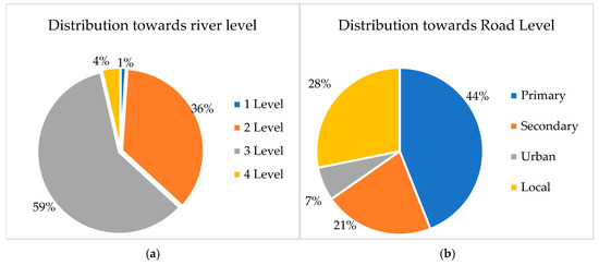
Figure 1.
Distribution of bridges towards river levels (a) and road levels (b).
In addition, considering the hierarchy of the bridges, it is possible to focus attention on the data in Figure 2. Bridges are also classifiable in terms of their overall length L (i.e., the sum of the longitudinal span of beams or arches). Establishing that a short-span bridge (SSB) has an L of <20 m (due to the fact that this is a length compatible with the ordinary transportation of prefabricated beams), a medium-span bridge (MSB) has an L of < 50 m, and a large-span bridge (LSB) has an L of >50 m, the Sardinian territory is characterized by the distribution highlighted in Figure 2a. Conversely, Figure 2b shows the density of inhabitants and infrastructures.
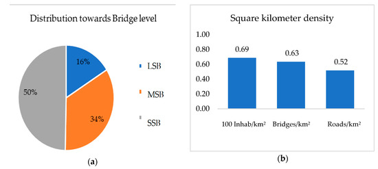
Figure 2.
Distribution of bridges towards bridge levels (a) and road levels (b).
The flood of October 2018 analysed in this work reveals the significant fragility of the territory, particularly with respect to the road network. Redundancy of the street system might succeed in reducing the impact of floods in terms of economic consequences.
In this sense, the safety assessment of SSBs is a combination of the mechanical parameters of a bridge [10] and structural collapse scenarios [11,12], especially the ones due to hydraulic action during flood events. Structural evaluations and computational design methods are discussed in [13,14]. Low-cost monitoring techniques and strategies for bridges are widely available in the literature [7,15,16,17]. These strategies are not systematically applied in ensuring efficient provisional or maintenance activity in the Italian and Sardinian contexts. Retrofitting is often performed only after a destructive event [18] or after damage causing the interruption of road traffic.
An engineering judgement approach suggests that this policy is not sustainable from a technical and economic point of view. This reveals a gap between the instruments available to stakeholders and the present state of the art of civil engineering. This work furnishes a contribution to this perspective. Section 2 reports a simple provisional framework to provide a limit analysis of SSBs [19]. Section 3 describes the application of this approach to an example in the case study area. In Section 4, the case study is discussed and analysed, highlighting the benefits and drawbacks of the framework.
2. Limit Analysis of SSB
With the aim of mitigating the hydrogeologic vulnerability of SSBs in secondary road networks, the following activities are proposed:
- (i)
- Classification of SSBs in terms of the mentioned level of relevance.
- (ii)
- Identification of safety levels for each SSB and alternative paths in the case of single or multiple collapses.
- (iii)
- Definition of effective practical solutions and maintenance operations to optimize the cost/benefit ratio for retrofitting investment.
These activities are devoted to assessing the limit damages with respect to secondary, urban, and local road networks and SSBs subjected to hydrogeologic hazards. This can be achieved, increasing quality levels as much as reasonably possible and equally minimizing the costs. The limited amount of data available with respect to a wide range of SSBs in urban or rural areas requires a procedure based on the following steps: (1) classification, (2) analysis, and (3) design.
2.1. Classification
The classification is based on a survey of territorial data. This can be carried out using the free QGIS 2.18 software, combined with an on-site survey. From a comparison with hydraulic and road cartographies, it is possible to quickly identify all intersections between these networks. The survey form proposed in [19] is reported in Figure 3.
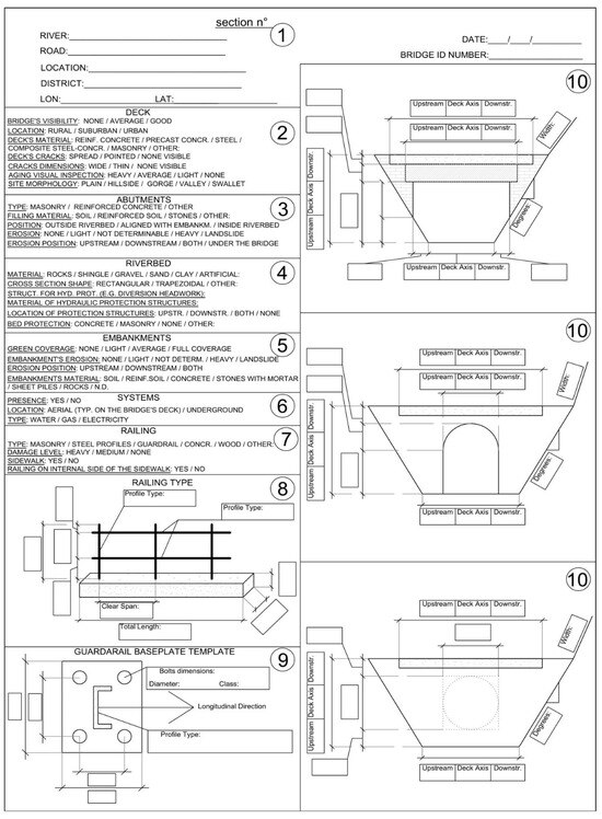
Figure 3.
Survey form [19].
Experiences in some Italian areas show that parts of the crossings derived from QGIS are not indicated in traditional maps; this means that they are unknown to public authorities and are thus unaccounted for in proper maintenance activities. Therefore, the QGIS screening should be followed by an in situ systematic survey. This can be carried out through the filling out of the specific form shown in Figure 3, which is specifically prepared to allow an easy and quick survey. Examples can be found in [9,20,21]. Geometric information on infrastructure can also be obtained by photogrammetry or drones. This is particularly convenient wherever accessibility is an issue. In some cases, point clouds or laser scanner analysis performed using an unmanned aerial vehicle (UAV) can help in the survey. In parallel, rainfall data can be easily obtained via QGIS using hydraulic data available from the regional authority.
2.2. Analysis
Provided that the crisis of the SSB structure is essentially due to hydraulic reasons, mainly caused by overtopping, erosion, or floating effects [9,22,23], an analysis of the peak discharge condition is compulsory. It is necessary to evaluate the maximum hydraulic capacity of the bridge in terms of flow rate and to compare it with the demand.
The maximum capacity of a bridge is influenced by the fact that the limit flow rate (in the case of free-flow conditions) depends on the water level in correspondence with the infrastructure (Figure 4). The maximum water level for the free-flow condition corresponds to the clearance of the bridge hb, named the critical height.
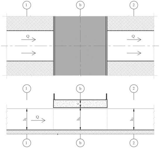
Figure 4.
A typical river section. Three main control sections are identified: (1) the upstream section, (b) the bridge section, and (2) the downstream section.
The proposed method based on the three steps (survey, analysis, and design) requires a geometric and geographical census of SSBs. This goal can be obtained following the scheme proposed in Figure 5. The aim is to quickly obtain information with an efficient and focused survey. Figure 5 highlights the main input parameters that can be measured with simple and cheap instruments used during the survey.
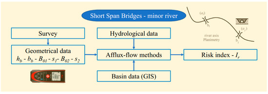
Figure 5.
Sketch of the proposed method of investigation.
Assuming a rectangular or trapezoidal hydraulic section (one of the most frequent shapes), the flow rate depends on the geometrical boundary conditions highlighted in Figure 4. The upstream section (1) is crucial in the case of slow flow rates, while the downstream one (2) is important in the case of fast flow rates. Assuming a section with a distance from the bridge (b) such that uniform flow is reached, the well-known Manning equation can be used:
in which
n denotes the Manning coefficient;
I0 denotes the river’s slope;
Ai denotes the area of the i-th section: upstream (1) or downstream (2);
Rmi denotes the hydraulic radius of the i-th section.
The area and the hydraulic radius are given by the following expression for trapezoidal shapes:
where
B0i denotes the minor base of the trapeze;
si denotes the embankment’s transverse slope;
yi denotes the liquid height.
Subscript i can assume a value of 1 or 2 according to Figure 4.
Applying the Bernoulli equation to section i and the section under the bridge (b), the following is obtained:
Combining (1) and (4), variables Q and y can be computed as follows:
From the system of Equation (5), it is possible to evaluate the maximum capacity of the bridge, which is called Qc from this point on, in which subscript c indicates the capacity.
2.3. Design
A rational formula is assumed to evaluate the peak discharge [24]:
where
k is a unit conversion factor (1/3.6 for the SI units);
C is the rational runoff coefficient;
S is the area of the water catchment in square kilometres;
i is the rainfall intensity (mm/h);
h is the height of the rain (mm);
Tc represents the concentration time (hour).
For small basins, Equation (6) furnishes a good estimation of the design’s flow rate [25]. The value of C can be obtained from the ratio between the volume of rainfall to the runoff, using the water balance equation combined with the curve number (CN) value to obtain the superficial outflow [26]. CN can be evaluated considering the land/soil use derived from the QGIS 2.18 freeware platform and properly averaged on the catchment area. As the antecedent moisture condition (AMC) represents a critical parameter for the CN, two values were computed, CNII and CNIII, to highlight variations in the peak discharge. Assuming the area of the catchment as a deterministic value, the main uncertainties in the use of Equation (6) are related to C, h, and Tc.
In the scientific literature, it is possible to find several expressions for Tc [24]:
in which the symbols used have the following meaning:
L—length of the river;
V—average speed of the hydraulic flow;
d—difference in altitude covered by the river;
ia—average slope of the basin.
Equation (7) proposed by Giandotti is well suited for large basins (170 < S < 70,000 km2). It was derived from several Italian rivers and can also be used for minor basins. Equation (8) suggested by Viparelli was derived from the study of Piedmont’s rivers. It is usually applied at flow speeds between 1.0 and 1.5 m/s. Equation (9) of Puglisi-Zanframundo is based on studies of small basins in the Apulian Apennines (7 < S < 200 km2). Even the D’Asario Equation (10) is valid for small basins (1 < S < 100 km2). The last equation, Equation (11), is attributed to Kiprich, and it is calibrated relative to very small basins (S < 0.4 km2). These expressions for TC are identified using a range of twelve expressions for the concentration time [27,28].
Nevertheless, Equations (7)–(11) furnish a wide variation range relative to Tc. Their application to the assumed case study provides an average value for the return period TCm equal to 6.2 h, with a standard deviation σ of 2.2 h. The effect of this large variation on the calculation of the design flow rate is hereafter considered, and it is shown in the graphs of Figure 5 and Figure 6. Qd is calculated for five values of the return period belonging to the range TCm ± γ∙σ (with γ = 0.0, √2/2, √2) in order to explore the variety of solutions given by Equations (7)–(11).
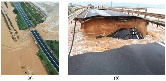
Figure 6.
First collapse: aerial view (a) and detail (b).
For basins with reduced areas, the use of Equation (6) is based on the hypothesis that the maximum flow rate value is obtained by a rainfall duration t equal to the concentration time Tc. Under this assumption, the concentration time in (6) is to be assessed carefully [29].
The height of rain in Sardinia can be expressed as follows [30]:
where
t is the duration of the rain.
a1 and b1 are empirical coefficients related to the site. Sardinia is divided into 7 districts characterized by several daily rain indexes (µg).
a2 and b2 are empirical coefficients that link rainfall to the return period of an event (Tr). Coefficient b2 has different values depending on the critical storm duration. The major distinction is between less than and higher than 1 h.
The coefficients a1, b1, a2, and b2, assumed in this study are listed in the following.
In this hydrologically homogeneous area (Campidano), the coefficient µg is 58 mm/day.
The critical storm duration to the peak discharge can be assumed to be equal to the concentration time for small basins, and Equation (6) becomes the following:
where
is a coefficient that is linked to specific sites. It depends on the daily rain index (µg) and soil permeability through C, while
is a coefficient related to the return period of the events (Tr).
Equation (10) allows a sensitivity analysis of the parameters that mostly affect the expression of the peak discharge. Hence, in the following histogram, the effect of the variation in the concentration time for rainfalls is evaluated and characterized by a different return period Tr. Considering the design return period, Equation (18) gives the peak discharge, defined from now on as the design flow rate Qd.
The method by which Qd is calculated deeply influences the results. Its sensitivity to the duration of the rain expressed by Equation (18) makes the flow rate essentially prone towards having a peak value relative to the so-called tropical rainfall. Indeed, recent climate change led to more frequent short-time rainfall with very high intensities. Hence, they have a dangerous influence on the peak discharges of small streams (rivers of the 3rd or 4th levels). All parameters are recommended in the regional document of Sardinia [30].
The evaluation of the capacity and design flow rate can be calculated by risk index Ir:
The comparison between Qc and Qd represents an overall indicator of the outflow capacity of infrastructure. This method, applied to a case study in the National Park of Metalliferous Hills [8] (Tuscany, Italy), highlighted that most SSBs exhibited an insufficient capacity [8]. This is a typical feature of such structures, and this approach clearly indicates that SSBs are particularly prone to flood risks. The analysis of this case study shows the key role of upstream and downstream vertical-section geometry. In this sense, a spreadsheet was prepared and used, furnishing Ir for several scenarios.
From a decision-making point of view, an engineer’s activity could be limited to monitoring the asset or making decisions for the implementation of an early warning system. Concerning the bridge itself, the policy could involve a reinforcement of the lateral barriers, a specific geotechnical study to consolidate the abutments, or a wider retrofitting measure of the entire bridge. A further aspect is the uncertainty relative to the open channel flows and the accuracy of the river’s cross-section in the case of small watercourses due to the costs of a systematic survey and their variability over time. The proposed method is then limited to a geometrical survey of the cross-section of bridges, neglecting the influence of embankments and the longitudinal section. Hence, this approach should be applied in specific sites (i.e., bridge locations). Thus, this framework does not provide continuous information regarding the river axis but only in correspondence to the infrastructure.
We also point out that the classic and well-known formulas used here are adopted in an innovative way to determine the risk index (21).
Finally, an exhaustive analysis of a stock of SSBs has to also involve traffic network analysis [31] and be able to discriminate roads with high traffic densities from those with lower vehicle densities.
3. The Sardinia Case Study
Heavy rainfall dated 10 October 2018 hit the Southern Sardinia in a few hours, causing floods in the area of Capoterra. The effects of this event led to the collapse of the approach ramp of a short-span bridge located on the SS 195 road. The water level in the pond rose until it exceeded the embankments. The water’s thrust was followed by the erosion of the backfill soil. No structural damage was inflicted on the structure of the bridge, but the approaching ramps were affected. The first collapse affected both lanes at km9 + 300 (Figure 6). A few hours later, another portion of the lane collapsed (Figure 7).
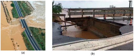
Figure 7.
Second collapse [31]: aerial view (a) and detail (b).
The Municipality of Capoterra covers an area of 68.25 km2. The rivers are Rio Santa Lucia (28 km length) and Rio San Girolamo (15 km length), together with a secondary hydraulic network (Figure 8), both originating from a surrounding set of hills measuring 500 m in height. The hydrogeological setting plan (PAI) classifies this area as “high hydraulic risk”.
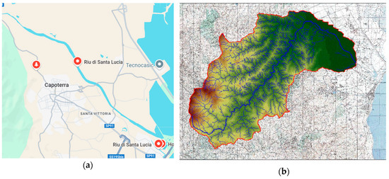
Figure 8.
Santa Lucia River: planimetry (a) and drainage basin (b) [30].
The drainage basin indicated short concentration times when strong rainfall occurred (Table 1).

Table 1.
Hydrological data of the Santa Lucia river [30].
Recent hydraulic defence structures regulate the river’s flow to prevent the inundation of settlements and infrastructure [32]. Nevertheless, it was not sufficient to avoid collapses due to floods. Figure 9 illustrates the daily distribution of rainfall in the first decade of October 2018. The peak during October 10th (465 mm) highlights the exceptional nature of the event [30].
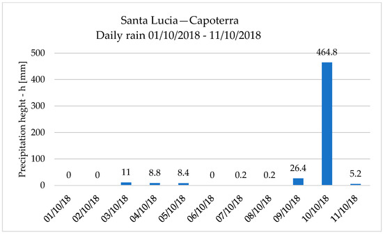
Figure 9.
Santa Lucia rain gauge station—distribution of daily precipitation in the days before flood.
Within 3 h, the corresponding rain gauge station recorded 183 mm of water (Figure 10). This amount considerably exceeds the historical maximums recorded during the last 25 years.
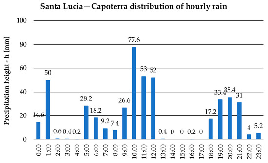
Figure 10.
Santa Lucia rain gauge station—distribution of hourly rain.
From a back analysis of historical rain data for the last 25 years, the annual cumulated rainfall oscillates between 50 and 200 mm [30].
3.1. Emergency Management Plan
Figure 11 illustrates both the fastest and alternative routes for reaching the city of Sarroch, where the main industrial oil plant of the area is located, producing most of the area’s car traffic. The estimated travel time was over 2 h after the flood event compared to 30 min using the fastest coastal route, which was available before the flood.
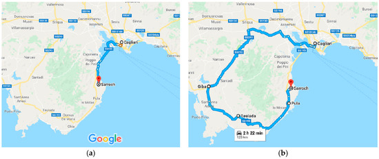
Figure 11.
Cagliari—Sarroch: itinerary before the collapse (a) and after the collapse (b) (Google Maps©).
As soon as the rain stopped, the emergency network rushed the repair operations of the collapsed approach ramps. This permitted the reopening of SS 195 after almost one week. Besides this, the event caused the loss of two human lives and an overall economic loss of millions of Euros. The overall collapses were located at two different sites: one near an SSB adjacent to a roundabout (point 1 of Figure 12) and the other near the abutments of another SSB (point 2 of Figure 12). The first one comprised the partial collapse of an access ramp (Figure 13a), whilst the second comprised the collapse of both ramps (Figure 13b and Figure 14a) and a complete interruption of the route.
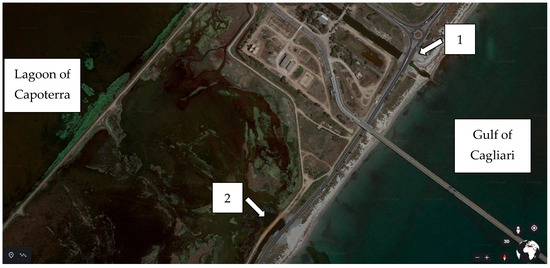
Figure 12.
Planimetric view of the two collapses of the case study (1) with minor damage and (2) major damage (GoogleEarth©).
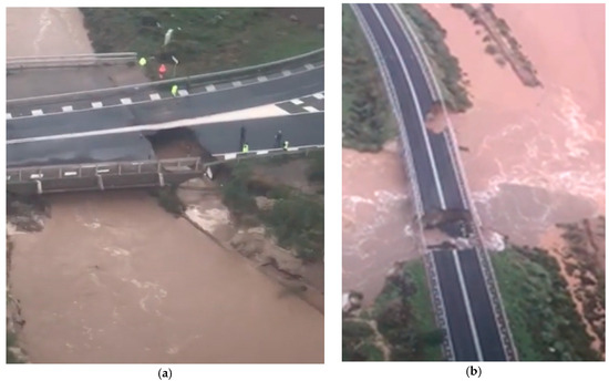
Figure 13.
Aerial view of the two collapses: (a) partial damage of an access ramp; (b) complete collapse of the southern ramp and partial damage of the northern one.
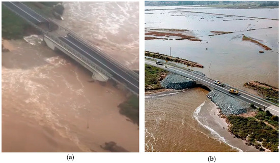
Figure 14.
Aerial views of bridge 2: (a) from the lagoon during the flood and (b) from the gulf after the reconstruction.
In both cases, an erosion effect occurred, and this was probably due to the insufficient flow capacity of the cross-section of the bridge, which was joined with weak backfill soil relative to the access ramps. The reconstruction, especially for bridge 2 in Figure 12, was targeted to mitigate this aspect (Figure 14b).
Bridge 2 comprises two-sided structures: a concrete-stone arch and a simply supported r.c. beam. The arch, visible from the sea gulf (Figure 15a), was built in 1927 using a lowered monocentric profile. The r.c. beam, visible from the pond (Figure 15b), was built in the 1980s to widen the road, as shown in Figure 16.
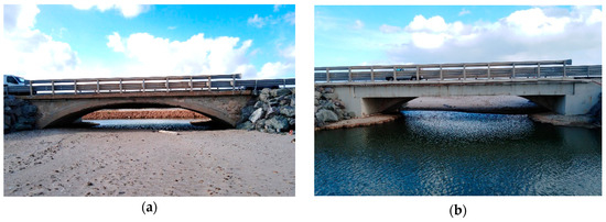
Figure 15.
Views after the reconstruction of bridge 2: (a) from the gulf; (b) from the lagoon.
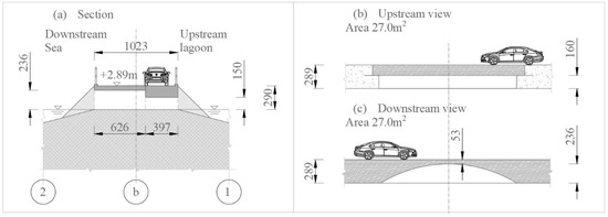
Figure 16.
Capoterra bridge: transversal section (a), upstream view, (b) and downstream view (c).
3.2. Analysis of the Capoterra Bridge
The framework described in Section 2.2 and Section 2.3 provides simple indications about the evaluation of the hydraulic capacity and demand of the infrastructure. The study of the catchment was carried out with QGIS (2.18—Las Palmas), and a weighted average value of CN was calculated to have a better estimation of C. The basin considered in the analysis comprises a section located about 10 km from the bridge, as shown in Figure 17. This allowed a direct comparison with the peak discharge obtained in [30].
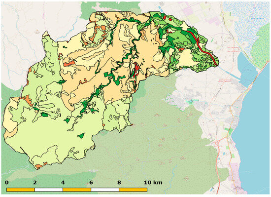
Figure 17.
Curve number map evaluated on the river catchment.
Equation (5) provides Qc. This represents the maximum capacity of the bridge in the case of free-flow rates (outflow liquid level equal to bridge clearance hb). Posing n as equal to 0.030 s/m1/3 and I0 = 0.002, it is possible to estimate a free-flow rate capacity equal to 49.4 m3/s. This corresponds to a mean flow velocity of 1.82 m/s in correspondence with the bridge, with the liquid height of free flows equal to 1.74m with respect to the upstream section. Qd is calculated with Equation (18), considering several return periods and rainfall durations (Figure 18) in the interval Tcm − 2ϒσ; Tcm + 2ϒσ. A significant variation in the rainfall duration relative to the design flow rate can be seen.
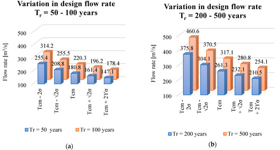
Figure 18.
Flow rate for a return period of 50–100 years (a) and 200–500 years (b).
The charts in Figure 18 represent the fact that the rainfall data related to different storm durations produce a considerable dispersion. Qd also varies by 41% with respect to the value calculated with the average Tcm value. This confirms the tropical shift of rainfall within the studied case area. Hence, overestimating TC in Equation (18) produces results that are not conservative. In fact, parameter C depends on the antecedent wetness condition of the soil: in the case of short heavy rainfall, soil saturation does not contribute to the runoff process due to its reduced imbibition capacity [33,34].
In Figure 19a, a comparison between design flow rate Qd and risk index Ir and the relative ones expected according to Table 2 (expected) is presented. Here, Qd is calculated with the average AMC condition (see Section 2.3). Two different Ir values are calculated with Equation (21) (Figure 19b) in order to compare the design flow rate proposed here (red) to the design flow rate expected in Table 2 (blue).
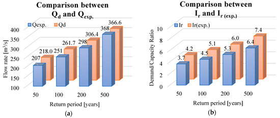
Figure 19.
Comparison between Qd and QExp (a) and Ir and IExp ratio (b).
Table 2.
Design (Qd) and expected (Qd) flow rate.
The expected flow rates (QExp) of Table 2 are in accordance with the design flow rates calculated using Equation (18). Qd produces a slightly greater effect than the expected discharge for all design return periods examined. This is valid for short return periods (Tr = 50 years; Qd = +5% and then QExp), while, for bigger ones (extraordinary flood events), the difference is negligible (Tr = 500 years; Qd = QExp).
The comparison between Qd and QExp flow rates is shown in Table 2. Soil imbibition produces differences in the range (−14%; +23%) relative to the expected flow rate. In the case of our design, the assumption of the most severe conditions (CN III—consistent precipitation during the previous 5 days) can appear severe for frequent rainfall: the average condition is recommended.
The structural capacity of the embankment of the bridge during free-flow conditions appears inadequate. Admitting a design flow rate of 200 m3/s (Tr = 50 years; QExp = 207.2 m3/s) with sufficient energy to pass under the bridge, runoff occurs with a velocity equal to 7.4 m/s, an exceptionally high speed for rivers near sea level. Such velocities may lead to the erosion of backfill soil.
A further exceptional atmospheric phenomenon occurred in Sardinia just 7 years before on November 18th, 2013 (cyclone Cleopatra). It caused rainfall discharges of 440 mm in a day. This event led to the overflow of various rivers, causing the death of 18 people and significant damage to the agriculture and livestock sector. The collapse of an emblematic bridge (the Monte Pino bridge) was studied in [33]: the embankment was eroded through a not-maintained metallic culvert, causing the collapse of a 50 m road.
4. Discussion
The presented hydrologic framework based on rainfall data (Section 2) is applied to the mentioned case study (Section 3). Some evidence from this approach is as follows:
- (1)
- The application of the procedure discussed here furnishes a simple tool for technicians in designing and checking SSBs in the case of extreme rainstorms. The literature analysis shows that their collapse is essentially related to hydraulic reasons [23]. The use of Equation (6) emphasizes the most relevant parameters that describe discharge phenomena.
- (2)
- Further evaluations were carried out with respect to the capacity of the infrastructure. Most of the existing infrastructure exhibits a lower capacity relative to the demands required in the case of hydraulic overlaps. This could lead to the failure of SSBs, as shown in [9,20]. Specifically considering the rainfall data of Sardinia Island [34], the events characterized by a minor return period result in more severe effects than expected for SSBs.
- (3)
- The method proposed in Section 2 can be implemented in urban and suburban areas in order to evaluate the role of the infrastructure network.
- (4)
- The hierarchy of the infrastructure [29] plays a relevant role in stakeholders’ decision-making processes. In the mentioned case study, the interruption of SS 195 led to an increase in the travel time between Cagliari and Sarroch of about 3.3 times. The distance increased from 30 km to 128 km (+327%), while travel times increased from 33 to 142 min (+330%), impacting over 2000 workers/day. These aspects can be mitigated by increasing the robustness of the road network.
- (5)
- Fast reconstruction is the most recurrent action in the management of the territory [35]. Restorations to ante-operam (usually ante-collapse) conditions are nowadays a biased approach. Fast retrofits should be programmed before the collapse event. Several strategies [22,35] are available to increase structural capacities [36,37]. However, the hydraulic capacity of the infrastructure, which was once proven to be insufficient, should be increased with the same priority.
- (6)
- Other recent failures call attention to the drafting of schedules, which, based on the recurring types of infrastructure, leads to fast capacity planning, especially for vulnerable areas [38,39,40]. This can be applied in the case of collapses rather than in preventive measures. Specifically, for access ramp collapses, it is possible to introduce metal culverts (road manholes), which increase the discharge capacity of the infrastructure, reducing the speed of fluids and, therefore, the possibility of erosion.
- (7)
- More recent flood models have been proposed to take into account the aspect of the resilience of infrastructures [41,42,43] or the presence of wooden debris during floods [44].
5. Conclusions
This paper once again focused attention on SSBs as one of the most recurring vulnerable elements of road networks. The damage scenario of SSBs is different than LSBs. Susceptibility to erosion plays a key role in this sense.
In SSBs, failure is essentially caused by hydraulic reasons. This induced the proposal of a rainfall-based method for the safety evaluation of SSBs. The effect of climate change can be taken into account in structural designs, such as [44,45,46]. The framework proposed here is easy to use and physically based. It is also possible to take into account the effects of climate change. Uncertainties related to the choice of concentration times, one of the main uncertain parameters, are examined here and discussed. Within this approach, it is possible to calculate the demand and capacity of an SSB and express its vulnerability through a risk index.
The framework is applied to the flood of Southern Sardinia that occurred in October, 2018. The insufficient hydraulic capacity of the collapsed bridge is highlighted. The natural event is also analysed considering the exceptional nature of the event and the implications in terms of traffic. The procedure proposed is compared with the data presented in the hydrological setting plan [30].
The analysis shows that a fast reconstruction to the before-collapse status is not sufficient for solving the problem. Some strategic retrofitting actions, such as increasing the hydraulic capacity of the infrastructure, should be taken into account. Further developments will be carried out in order to improve this method. In particular, economic losses shall be considered in the framework, together with the hierarchy of the infrastructure. Finally, proper management strategies with respect to the low-cost monitoring of bridges can help the optimization of economic investments with respect to these types of infrastructure.
Author Contributions
All the authors contributed to writing this paper. M.L.P. and M.S. conceived the method and carried out the case study. A.P. developed the GIS analysis and contributed to the related calculations. All authors have read and agreed to the published version of the manuscript.
Funding
This work was partly financed by FEDER funds through the Competitivity Factors Operational Programme—COMPETE and by national funds through the FCT Foundation for Science and Technology within the scope of the project POCI-01-0145-FEDER-007633. Moreover it was financed by Italian Ministry of University Research (PRIN 2020 S-MoSES) and Italian Ministry of Infrastructures and Transportations (RELUIS CSLLPP).
Acknowledgments
We thank PRIN 2020 S-MoSES (Italian Ministry of University Research) and RELUIS CSLLPP (Italian Ministry of Infrastructures and Transportations) for their support. We also thank the Agency of Sardinia Region for the data.
Conflicts of Interest
The authors declare no conflicts of interest.
References
- Ryan, D.; Ettema, R.; Solan, B.; Hamill, G. Stability of Short-Span Bridges Subject to Overtopping during Floods: Case Studies from UK/Ireland and the USA. In Proceedings of the 36th IAHR World Congress, Hague, The Netherlands, 28 June–3 July 2015; pp. 1–11. [Google Scholar]
- Puppio, M.L.; Novelli, S.; Sassu, M. Failure evidences of reduced span bridges in case of extreme rainfalls the case of Livorno. Frat. Integrita Strutt. 2018, 12, 190–202. [Google Scholar]
- Haines, A.; Kovats, R.S.; Campbell-Lendrum, D.; Corvalan, C. Climate change and human health: Impacts, vulnerability and public health. Public Health 2006, 367, 2101–2109. [Google Scholar]
- Huizinga, J.; De Moel, H.; Szewczyk, W. Global Flood Depth-Damage Functions: Methodology and the Database with Guidelines; Publications Office of the European Union: Luxembourg, 2017; ISBN 9789279677816. [Google Scholar]
- Stochino, F.; Mistretta, F.; Mancini, G.; Pani, L. Structural assessment and retrofitting of damaged reinforced concrete water bridge. In Proceedings of the 20th Congress of IABSE 2019 New York City The Envolving Metropolis, New York, NY, USA, 4–6 September 2019; pp. 1477–1485. [Google Scholar]
- Stochino, F.; Bedon, C.; Sagaseta, J.; Honfi, D. Robustness and resilience of structures under extreme loads. Adv. Civ. Eng. 2019, 2019, 4291703. [Google Scholar]
- Titi, A.; Biondini, F.; Frangopol, D.M. Cost-based recovery processes and seismic resilience of aging bridges. In Maintenance, Monitoring, Safety, Risk and Resilience of Bridges and Bridge Networks, Proceedings of the 8th International Conference on Bridge Maintenance, Safety and Management IABMAS 2016, Foz do Iguaçu, Brazil, 26–30 June 2016; Bittencourt, T.N., Frangopol, D.M., Beck, A.T., Eds.; CRC Press: Boca Raton, FL, USA, 2016; pp. 198–205. [Google Scholar]
- Novelli, S. Collapse Scenarios of Short Span Bridges for Extreme Climate Events in Colline Metallifere Area. Master’s Thesis, University of Pisa, Pisa, Italy, 2017. (In Italian). [Google Scholar]
- Puppio, M.L. Safety Assessment and Strenghtening of Short Span Bridges in Case of Extreme Rainstorms. Ph.D. Thesis, University of Pisa, Pisa, Italy, 2018. [Google Scholar]
- Alecci, V.; Stipo, G.; La Brusco, A.; De Stefano, M.; Rovero, L. Estimating elastic modulus of tuff and brick masonry: A comparison between on-site and laboratory tests. Constr. Build. Mater. 2019, 204, 828–838. [Google Scholar] [CrossRef]
- Casapulla, C. On the resonance conditions of rigid rocking blocks. Int. J. Eng. Technol. 2015, 7, 760–771. [Google Scholar]
- Casapulla, C.; Maione, A. Free damped vibrations of rocking rigid blocks as uniformly accelerated motions. Int. J. Struct. Stab. Dyn. 2016, 17, 1750058. [Google Scholar] [CrossRef]
- Casapulla, C.; Mousavian, E.; Zarghani, M. A digital tool to deisgn structurally feasible semi-circular masonry arches composed of interlocking blocks. Comput. Struct. 2019, 221, 111–126. [Google Scholar] [CrossRef]
- Alecci, V.; Briccoli Bati, S.; Ranocchiai, G. Numerical homogenization techniques for the evaluation of mechanical behaviour of a composite with SMA inclusions. J. Mech. Mater. Struct. 2009, 4, 1675–1688. [Google Scholar]
- Mistretta, F.; Piras, M.V.; Fadda, M.L. A reliable visual inspection method for the assessment of r.c. structures through fuzzy logic analysis. In Proceedings of the 4th International Symposium on Life-Cycle Civil Engineering, IALCCE, Tokyo, Japan, 16–19 November 2014; Taylor & Francis Group: Abingdon, UK, 2014; pp. 1154–1160. [Google Scholar]
- Fadda, M.L.; Mistretta, F.; Piras, M.V. Vulnerability assessment of concrete bridges using different methods of visual inspection. In Proceedings of the Civil-Comp Proceedings, Civil-Comp Press, Naples, Italy, 30 June 2014; Volume 105. [Google Scholar]
- Porcu, M.C.; Patteri, D.M.; Melis, S.; Aymerich, F. Effectiveness of the FRF curvature technique for structural health monitoring. Constr. Build. Mater. 2019, 226, 173–187. [Google Scholar]
- Tattoni, S.; Stochino, F. Collapse of prestressed reinforced concrete jetties: Durability and faults analysis. Case Stud. Eng. Fail. Anal. 2013, 1, 131–138. [Google Scholar] [CrossRef]
- Pucci, A.; Puppio, M.L.; Giresini, L.; Sousa, H.; Matos, J.C.; Sassu, M. Method for sustainable large-scale bridges survey. In Proceedings of the Towards a Resilient Built Environment Risk and Asset Management, Guimarães, Portugal, 27–29 March 2019; pp. 1034–1041. [Google Scholar]
- Mistretta, F.; Sanna, G.; Stochino, F.; Vacca, G. Structure from motion point clouds for structural monitoring. Remote Sens. 2019, 11, 1940. [Google Scholar] [CrossRef]
- Sassu, M.; Giresini, L.; Puppio, M.L. Failure scenarios of small bridges in case of extreme rainstorms. Sustain. Resilient Infrastruct. 2017, 9689, 108–116. [Google Scholar] [CrossRef]
- Stochino, F.; Fadda, M.L.; Mistretta, F. Assessment of RC Bridges integrity by means of low-cost investigations. Fract. Struct. Integr. 2018, 12, 216–225. [Google Scholar] [CrossRef]
- Milano, V. Introduction to Hydrography and Hydrology; TEP Editor: Pisa, Italy, 2016. (In Italian) [Google Scholar]
- Young, C.B.; Mcenroe, B.M. Evaluating the Form of the Rational Equation. J. Hydrol. Eng. 2014, 19, 265–269. [Google Scholar] [CrossRef]
- Chow, V.T.; Maidment, D.R. Applied Hydrology; McGraw-Hill: New York, NY, USA, 1988. [Google Scholar]
- Edgar Watt, W.; Ander Chow, K.C. A general expression for basin lag time. Can. J. Civ. Eng. 1985, 12, 294–300. [Google Scholar] [CrossRef]
- Salimi, E.T.; Nohegar, A.; Malekian, M.; Hoseini, M.; Holisaz, A. Estimating time of concentration in large watersheds. Paddy Water Environ. 2017, 15, 123–132. [Google Scholar] [CrossRef]
- Efstratiadis, A.; Koussis, A.D.; Koutsoyiannis, D.; Mamassis, N. Flood design recipes vs. reality: Can predictions for ungauged basins be trusted ? Nat. Hazards Earth Syst. Sci. 2014, 14, 1417–1428. [Google Scholar] [CrossRef]
- AA.VV. Guide Lines of Pluviometric Probability; Presidenza Del Consiglio Dei Ministri—Dipartimento Per I Servizi Tecnici Nazionali: Pisa, Italy, 2006; p. 228. (In Italian)
- Municipality of Capoterra. Civil Protection Plan Application for Hydraulic Risk 2015. Capoterra, Italy. (In Italian)
- Italian Ministry of Infrastructures and Transportations. Geometric Functional Rules for Road Construction; Ministero delle Infrastrutture e dei Trasporti: Rome, Italy, 2001; Volume 285, p. 90. (In Italian) [Google Scholar]
- Giresini, L.; Puppio, M.L.; Sassu, M. Collapse of corrugated metal culvert in Northern Sardinia: Analysis and numerical simulations. Spec. Issue Int. J. Forensic Eng. 2016, 3, 69–85. [Google Scholar] [CrossRef]
- Montrasio, L.; Valentino, R.; Losi, G.L. Rainfall-induced shallow landslides: A model for the triggering mechanism of some case studies in Northern Italy. Landslides 2009, 6, 241–251. [Google Scholar] [CrossRef]
- Deidda, R.; Piga, E.; Sechi, G.M. Regional Analysis of Frequency of Intense Rainfalls in Sardinia; Technical Report from Regional Hydrological Office; IWA Publishing: London, UK, 2020. (In Italian) [Google Scholar]
- Piras, M.V.; Deias, L.; Mistretta, F. Vulnerability analysis of a reinforced concrete structure by visual inspection. In Bridge Maintenance, Safety, Management and Life-Cycle Optimization, Proceedings of the 5th International Conference on Bridge Maintenance, Safety and Management, Philadelphia, PA, USA, 11–15 July 2010; Taylor & Francis Group: Oxfordshire, UK, 2010; pp. 2045–2050. [Google Scholar]
- Biondini, F.; Frangopol, D.M. Design, assessment, monitoring and maintenance of bridges and infrastructure networks. Struct. Infrastruct. Eng. 2015, 11, 413–414. [Google Scholar] [CrossRef]
- Frangopol, D.M.; Biondini, F. Bridge design, maintenance and management. Struct. Infrastruct. Eng. 2014, 10, 419. [Google Scholar]
- Santarsiero, G.; Picciano, V.; Masi, A. Structural rehabilitation of half-joints in RC bridges: A state-of-the-art review. Struct. Infrastruct. Eng. 2023, 21, 227–250. [Google Scholar] [CrossRef]
- Santarsiero, G.; Picciano, V.; Masi, A.; Ventura, G. Retrofit of PRC bridges by external post-tension under different corrosion scenarios. In Bridge Maintenance, Safety, Management, Digitalization and Sustainability, Proceedings of the 12th International Conference on Bridge Maintenance, Safety and Management, IABMAS 2024, Copenhagen, Denmark, 24–28 June 2024; CRC Press: Boca Raton, FL, USA, 2024; pp. 571–579. [Google Scholar] [CrossRef]
- Picciano, V.; Santarsiero, G.; Masi, A.; Ventura, G. Review and analysis of RC bridge half-joints strengthening techniques. Procedia Struct. Integr. 2024, 62, 1020–1027. [Google Scholar]
- Croce, P.; Formichi, P.; Landi, F. Assessment of long-term structural reliability considering climate change effects. In Proceedings of the IABSE Congress Ghent 2021—Structural Engineering for Future Societal Needs, Ghent, Belgium, 22–24 September 2021; pp. 52–60. [Google Scholar]
- Croce, P.; Formichi, P.; Landi, F. Probabilistic methodology for the assessment of the impact of climate change on structural safety. In Proceedings of the 30th European Safety and Reliability Conference, ESREL 2020 and 15th Probabilistic Safety Assessment and Management Conference, PSAM 2020, Venice, Italy, 1–5 November 2020; pp. 4758–4764. [Google Scholar]
- Croce, P.; Formichi, P.; Landi, F. Implication of climate change on climatic actions on structures: The update of climatic load maps. In Proceedings of the IABSE Symposium: Synergy of Culture and Civil Engineering—History and Challenges, 1st IABSE Online Symposium, IABSE Symposium Wroclaw 2020, Wroclaw, Poland, 7–9 October 2020; pp. 877–884. [Google Scholar]
- Tubaldi, E.; White, C.J.; Patelli, E.; Mitoulis, S.A.; De Almeida, G.; Brown, J.; Cranston, M.; Hardman, M.; Koursari, E.; Lamb, R.; et al. Invited perspectives: Challenges and future directions in improving bridge flood resilience. Nat. Hazards Earth Syst. Sci. 2022, 22, 795–812. [Google Scholar] [CrossRef]
- Kosic, M.; Anžlin, A.; Bau, V. Flood Vulnerability Study of a Roadway Bridge Subjected to Hydrodynamic Actions, Local Scour and Wood Debris Accumulation. Water 2023, 15, 129. [Google Scholar]
- Buka-Valvade Nicoletti, V.; Gara, F. Advancing bridge resilience: A review of monitoring technologies for flood-prone infrastructure. Open Res. Eur. 2025, 5, 26. [Google Scholar] [CrossRef]
Disclaimer/Publisher’s Note: The statements, opinions and data contained in all publications are solely those of the individual author(s) and contributor(s) and not of MDPI and/or the editor(s). MDPI and/or the editor(s) disclaim responsibility for any injury to people or property resulting from any ideas, methods, instructions or products referred to in the content. |
© 2025 by the authors. Licensee MDPI, Basel, Switzerland. This article is an open access article distributed under the terms and conditions of the Creative Commons Attribution (CC BY) license (https://creativecommons.org/licenses/by/4.0/).