Article

Simplified Impact Load Model Analysis of Vehicle-to-Bridge Pier Collision

1
Prime AE Group, Inc., Formerly Research Assistant, Bridge Engineering Software & Technology (BEST) Center, University of Maryland, College Park, MD 20742, USA
2
Bridge Engineering Software & Technology (BEST) Center, University of Maryland, College Park, MD 20742, USA
*
Author to whom correspondence should be addressed.
Infrastructures 2025, 10(12), 320; https://doi.org/10.3390/infrastructures10120320
Submission received: 16 October 2025 / Revised: 13 November 2025 / Accepted: 17 November 2025 / Published: 24 November 2025

Abstract

As a key member of the bridge substructure, the pier is always the most critical part under a variety of hazards, among which vehicle-induced impact is a rare but extreme load hazard that may result in significant structural damage and even the full failure of the bridge. Current design provisions, such as those in the AASHTO Load and Resistance Factor Design (LRFD) Bridge Design Specifications, adopt a constant equivalent static force (ESF) of 600 kips to represent vehicle impact loads. However, this simplified assumption neglects key parameters—such as vehicle speed, mass, and pier geometry—that significantly influence impact behavior. This study develops and evaluates two simplified impact load estimation models to improve the accuracy and practicality of design-level assessments: a reduced-order dynamic model and a response surface model. The reduced-order dynamic model captures vehicle–pier interaction through a simplified mass–spring system, while the response surface model uses regression-based relationships derived from extensive finite element (FE) simulations conducted in LS-DYNA. Sensitivity analyses identify the most influential parameters governing impact loads, including vehicle velocity, cargo mass, pier diameter, and impact height. The results show that both models can effectively predict peak dynamic and equivalent static impact loads, providing more accurate and physically interpretable results than the current constant-load approach. The proposed frameworks offer practical tools for bridge engineers to evaluate vehicle–pier collision scenarios and can be further extended for use in truck-to-pier and ship-to-pier impact analyses.

1. Introduction/Literature Review

As a critical component of the bridge substructure, the pier is one of the most vulnerable elements under various hazards. Among these, vehicle-induced impacts represent a relatively rare but extreme loading condition that can cause severe structural damage or even total bridge collapse [1]. Numerous technical reports and research studies have been conducted to better understand and improve the impact-resistant design of bridge piers. To summarize the current state of knowledge and design practices concerning vehicle–pier collision mechanisms, the following key literature was reviewed.

1.1. Codes

As specified in Art. 3.6.5, AASHTO LRFD code [2], the equivalent load was adjusted to 600 kips for the vehicle impact, and the location used to apply the load was moved to 5ft. above the ground. The orientation of impact is assumed to act in the direction of 0 to 15 degrees with the edge of the pavement in a horizontal plane. This revision is based on the latest crash tests of rigid columns impacted by 80-kip tractor–trailers at 50 mph [3]. Field observation indicates that shear failures are the primary mode of failure for individual columns, and columns that are 30in. in diameter or smaller are the most vulnerable.
However, the vehicular impact load specified in the code is still general compared with the force induced by ship collision in Article 3.14.8. The ship collision force clearly states the relationship with the mass and velocity of a vessel:
P s = 8.15 V D W T            
where P s is the equivalent static vessel impact force; D W T is the deadweight tonnage of the vessel; V is the impact velocity.
Compared with the ship collision force, the current vehicle collision force cannot present the relationship with the speed and mass of the vehicle. Furthermore, because the process of impact involves a complicated coupling mechanism of two systems, any parameter change in one system may lead to a different resultant impact load. The mass and stiffness contributions of both the superstructure and substructure should be taken into consideration to produce a more convincing result.
In Code ASCE7-10, although no impact load for the pier is specified, an equivalent static horizontal on a barrier system with 6000 lbf is listed [4]. However, this value is much lower than the AASHTO LRFD specification.
Appendix B of the European code Part 1-1 presents the impact of a vehicle on a barrier within a 1.5 m range as follows [5]:
F = 0.5 m v 2 / ( δ c + δ b )
where m is the gross mass (kg) of the vehicle; v is the velocity (m/s) of the vehicle normal to the barrier;   δ c is the deformation (mm) of the vehicle; and δ b is the deformation (mm) of the barrier. For vehicles not exceeding 2500 kg in weight, when applying this equation, the following values could be used to determine the force F: m = 1500 kg; v = 4.5 m/s; δ c = 100 mm. For rigid collision, δ b could take a value of zero. F then takes the value 152 kN (34.2 kips), which is also much smaller than the specification in the AASHTO.
Parts 1–7 of the European code give an equivalent static impact load up to 1000 kN (225 kips) in the parallel direction and 500 kN (112.5 kips) normal to the orientation of the road adjacent to the pier [6]. This value is closer to the AASHTO value but still underestimated. Appendix C suggests an alternative method for evaluating the impact load using the following equation:
F = v k m
where v is the impact velocity; k is the equivalent elastic stiffness of the object; m is the mass of the colliding object. This equation gives a more reasonable estimate of the impact, according to Ferrer’s study [7].
Therefore, there is a need for studies that comprehensively investigate the effects of truck weight, impact velocity, and pier properties in order to develop a generalized equation for estimating collision loads that incorporates these governing parameters.

1.2. Numerical Studies

El-Tawil [8] studied the dynamic performance of a single pier with either a rectangular or circular section subjected to the impact from a Chevrolet C2500 [9] and F800 Ford single-unit truck [10]. Consolazio and Cowan [11] built a 3D model of a double-column pier with a bent, foot, and piles. A simplified model, containing an SDOF barge system coupled with an MDOF pier system, was suggested, and its results were compared with the finite element solution. The suggested simplified method can efficiently evaluate the dynamic force.
Ferrer [7] conducted a simulation of a collision between a C2500 pickup truck and H-shape column. The simulation results showed that the static load equivalent to an impact was strongly dependent on the speed of the impacting vehicle. Buth [3,12] simulated the collision events of a single-unit truck weighing 65,000 lb and a tractor–trailer weighing 80,000 lb crashing into a rigid circular pier. Liu [13] started by simulating the impact test conducted by Fujikake et al. [14]. The F800 truck model developed by the National Crash Analysis Center for crash simulation with a concrete barrier (2005) was adopted to realize the collision simulation between a median-weight truck and a square pier. With a full composite jacket under 70 mph impact velocity, only minor damages were caused to the pier. Mohammed [15] investigated the behavior of a single hammerhead pier column under impact load induced by the C2500 pickup truck and F800 single-unit truck.
Gomez [16] performed a parametric study on an F800 single-unit truck crash into a circular pier with a 900 mm diameter. Damage ratios, calculated by dividing the peak dynamic impact force by the shear capacity of the pier, can be used to design bridge piers for specific damage states resulting from vehicle collisions. Abdelkarim et al. [17] studied the performance of hollow-core FRP–concrete–steel bridge columns subjected to vehicle collision. The peak dynamic force of the HC-FCS column was lower than that of the RC column. A 60 K E equation was used to estimate the equivalent static force, where K E is the kinetic energy of the vehicle.
Chen [18] ran finite element simulations to investigate the structural demands generated by an F800 colliding with a bridge pier. Do et al. [19] conducted a numerical simulation of the F800 single-unit truck crashing into a square-shaped pier. All three simplified models can predict the impact force well, whereas the beam model and the lumped mass model can obtain good displacement results that are close to those of the 3D full-scale model.
Alomari and Linzell [20] conducted comprehensive three-dimensional finite element simulations of intact, fire-damaged, and CFRP-retrofitted reinforced concrete bridge columns, demonstrating that the AASHTO-specified ESF may either underestimate or overestimate actual impact demands depending on vehicle speed, mass, and column properties.
Their work, together with earlier FHWA investigations, highlighted the need for more refined, parameter-dependent models that can better represent the dynamic nature of vehicular impacts. These findings motivate the present study, which develops and evaluates simplified yet physically based approaches to estimate impact loads and equivalent static forces for bridge piers.

2. Finite Element Analysis

A finite element analysis (FEA) was conducted to establish a foundation for developing the proposed simplified load models. The modeling and validation procedures followed the methodology presented in the preliminary study by Xu [21]. All analyses were performed in LS-DYNA@ (R7.0.0). The finite element analysis was validated by simulating the drop hammer test conducted by Fujikake et al., as shown in Figure 1. The same material properties, element types, and analysis controls used for the pier model were adopted to model the reinforced concrete (RC) beam in this validation. The concrete was modeled using 8-node, constant-stress, single-point integration solid hexahedral elements (MAT 159), while the steel reinforcement was represented by two-node Hughes–Liu beam elements with cross-section integration and 2 × 2 Gaussian quadrature (MAT 24). The beam element nodes were merged with the corresponding concrete solid element nodes to ensure full bond interaction without relative slip between steel and concrete. The drop hammer was modeled using 8-node, constant-stress, single-point integration solid elements (MAT 20), simplified as a rigid sphere with a radius of 90 mm. The static and dynamic coefficients of friction between the hammer and beam were set to 0.5 and 0.3, respectively, and an exponential decay coefficient of 0.001 was applied for velocity (in mm/s, equivalent to 1.0 for m/s). An automatic surface-to-surface contact algorithm was defined between the rigid hammer (master surface) and the beam (slave surface). The initial time step was set to 10-7 s. A time interval of 0.1 ms was used for the collection of data on the resultant contact forces.
From the time history of the impact force, the analytic curves maintained good agreement with the experimental curve for around the first peak response, which is also the maximum dynamic response yielded during the initial contact, as shown in Figure 2.
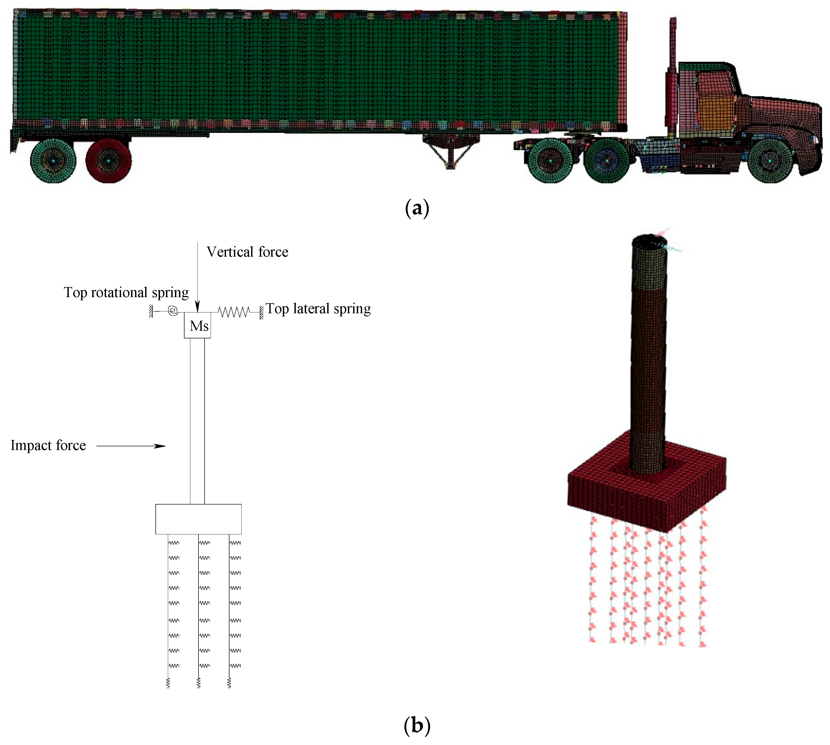
For the coupling system consisting of a vehicle and a pier, the vehicle is much more intricate than the pier. The tractor–trailer model [22] from National Crash Analysis Center (NCAC) was utilized in the analysis for the truck model. The pier and footing model are based on the Maryland structural detail manual 02-04. The impact height is controlled by the distance from the ground to the foot of the pier, which means that there is a higher impact location with a deeper pier foot. The superstructure is simplified into a lateral spring and a rotational spring to represent the restraint to the pier. The mass of the superstructure is lumped at the top of the pier. And the vertical force is used to simulate the reaction force supporting the superstructure. The column diameter is taken as 0.914 m (3′–0′′). The soil spring is spaced at every 457.2 mm (1′–6′′) with a lateral spring stiffness of 2.974 × 10³ N/mm, vertical spring stiffness of 6.637 × 10⁴ N/mm, and tip point spring stiffness of 1.009 × 10⁵ N/mm, respectively. The stiffness of springs was calculated using the approaches recommended by Greimann and wolde-Tinsae [23] by assuming an undrained cohesion of clay soil with 98.35 kPa (2054 psf). The plastic behaviors of piles are not taken into consideration.
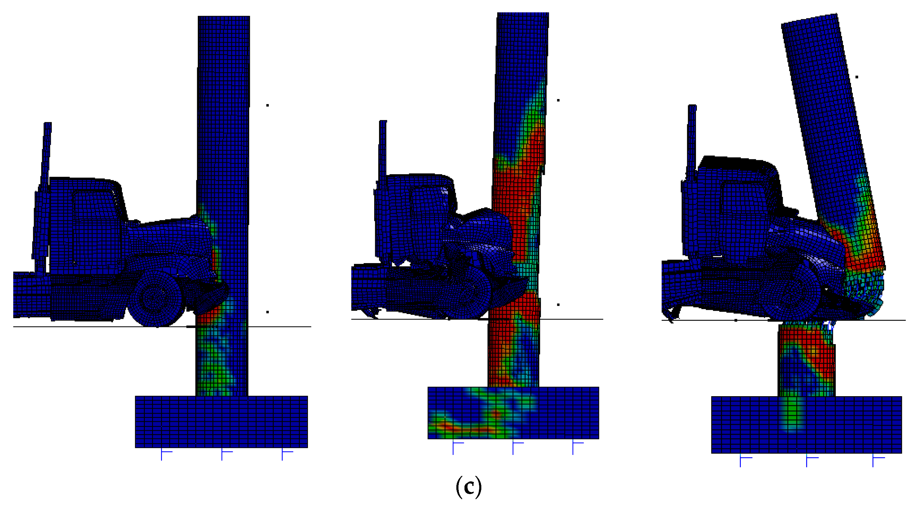
The finite element analysis results of the tractor–trailer are used for a comparison with the simplified model in the following sections. The finite element analysis model is shown in Figure 3. The results clearly illustrate the distinct failure mechanisms observed when a tractor–trailer truck collides with the pier—bending failure occurs at lower impact speeds, whereas shear failure becomes dominant at higher speeds. These observations provide important insight for the development of simplified impact load models, as they highlight the need to account for different structural responses under varying collision velocities when formulating generalized impact load equations.
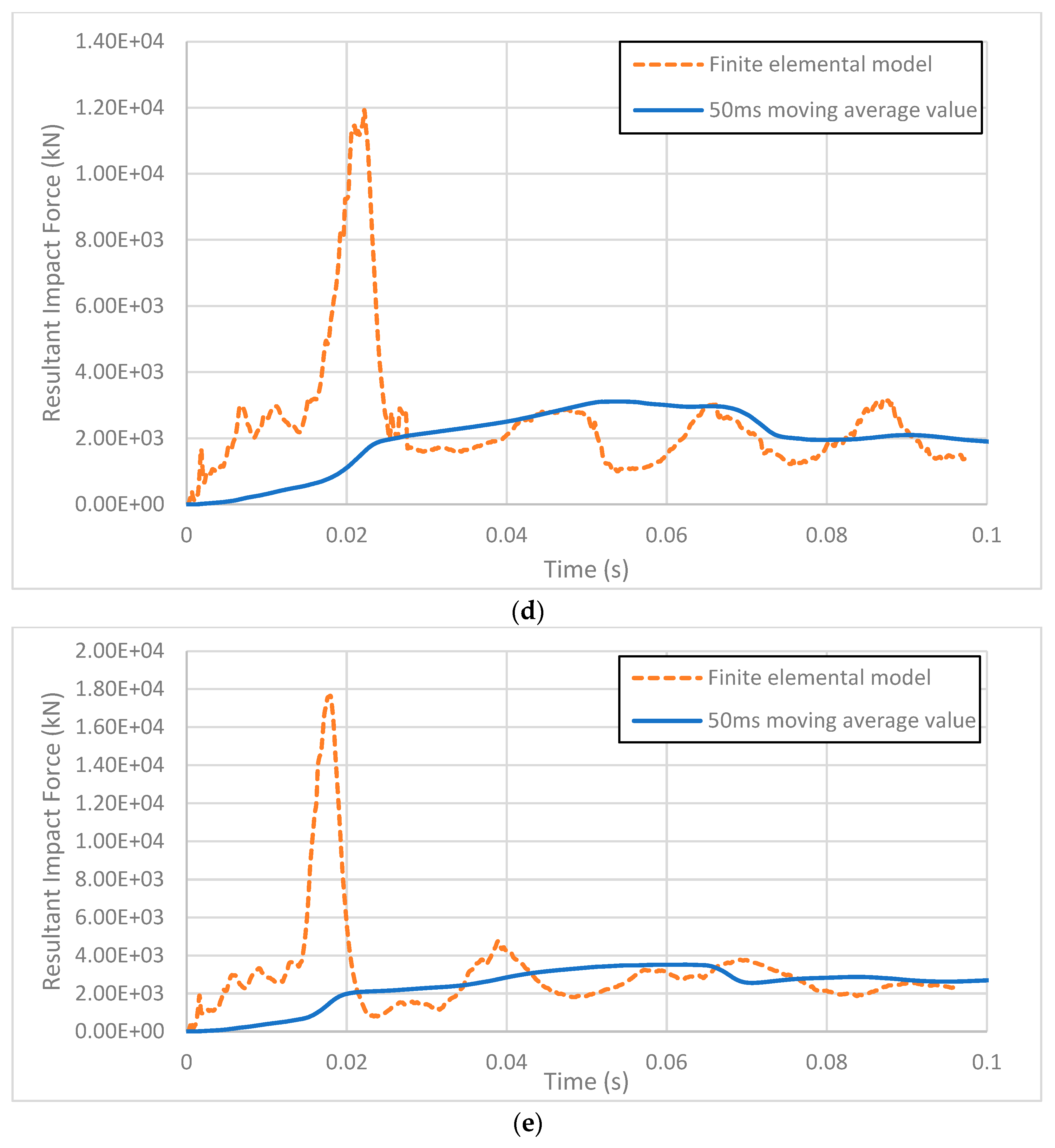
In addition to the dynamic impact load, the equivalent static load was employed to facilitate comparison with the design value recommended in the AASHTO LRFD specifications, following the approach outlined in FHWA Report 9-4973-2 [3]. This report recommends using the 50 ms average of the dynamic impact force to determine the equivalent static impact load. The present results show that the 50 ms averaged impact force agrees well with the 600-kip impact load suggested in the FHWA report, which was also adopted by the AASHTO LRFD Bridge Design Specifications.
Based on the finite element results presented in Table 1 and Table A1, the equivalent static loads can reach values as high as approximately 3500 kN for vehicle speeds of 120 km/h. These results are generally comparable to, and in several cases slightly exceed, the constant 600-kip (2669 kN) design load specified in the AASHTO LRFD. This comparison suggests that while the AASHTO provision offers a conservative and simplified representation of impact effects, it may underestimate load demands under high-speed impact scenarios, highlighting the need for more refined models in such conditions.

3. Simplified Load Model for Vehicle-Induced Impact

Conducting a finite element analysis on the vehicle-to-bridge pier collision problem is complicated, and case-by-case analysis is needed for different bridge piers under different vehicle impact models, which raises the need for a simplified impact load calculation method for structural engineers to easily handle the impact load based on their needs, even without the help of finite element software.
In this section, two simplified impact load methods will be discussed to show their feasibility in obtaining the required impact loads with respect to different cases.
(1)
Impact Load Model Based on Reduced-Order Dynamic Model

3.1. Assumptions of Reduced-Order Dynamic Model

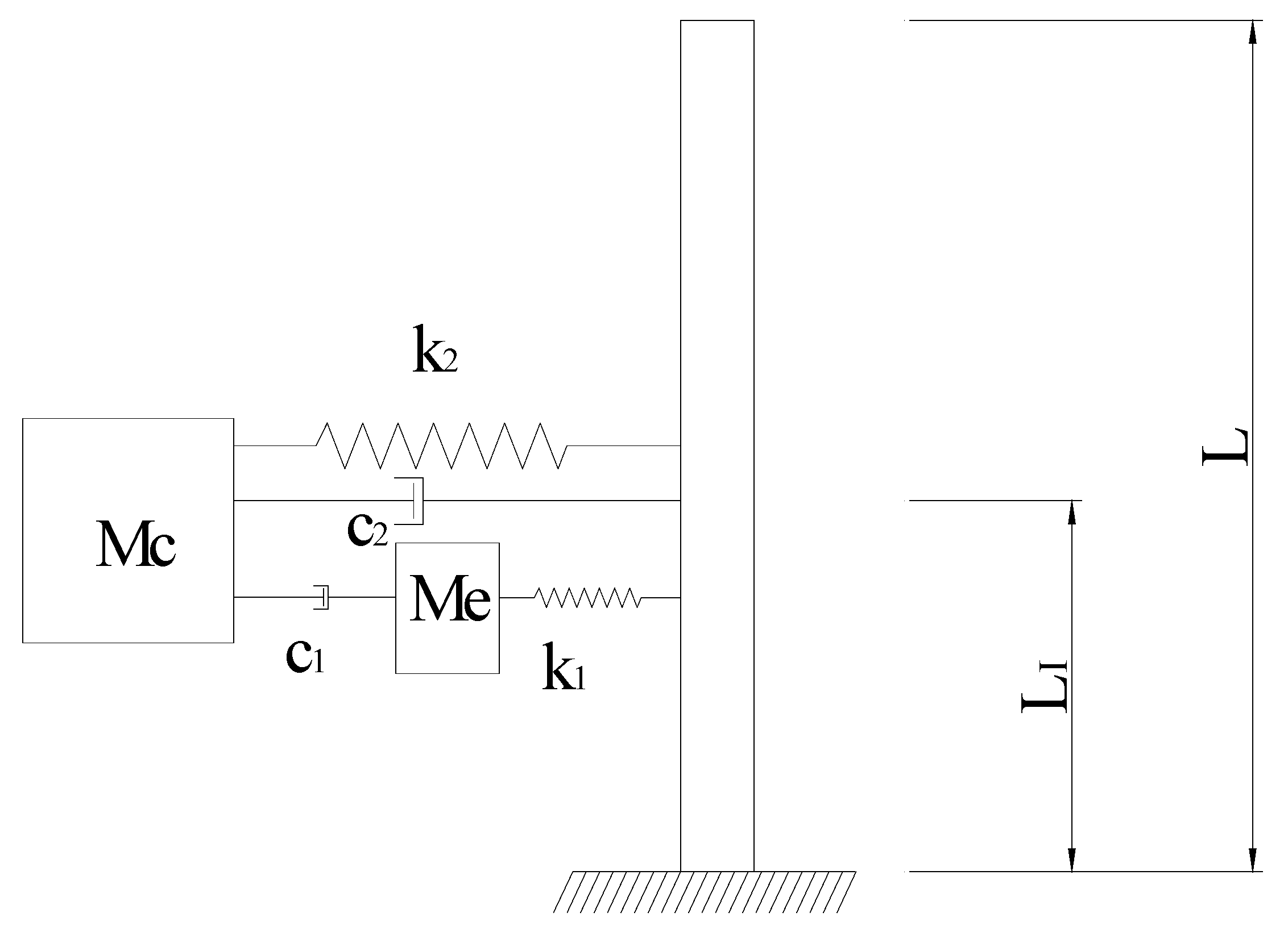
A preliminary study was conducted to evaluate the effect of lateral spring stiffness on the overall impact response, using values of 0.744 × 10³ N/mm, 1.487 × 10³ N/mm, and 2.974 × 10³ N/mm. The results indicated that the impact load is only marginally sensitive to the boundary stiffness of the bridge pier. Therefore, consistent with previous research [8], the truck–bridge impact system can be reasonably simplified into a mass–spring–pier model, as illustrated in Figure 4.

3.2. Vehicle Model

Me and Mc represent the engine and the rest of the vehicle, respectively. c1 represents the damping between the engine and vehicle due to deformation and compression during the impact. k1 simplifies the impact between the engine and pier into the spring under compression to simulate the contact mechanism. Similarly, c2 represents the damping between the rest of the vehicle and pier due to plastic deformation and the crushing of the soft covering of the vehicle during the impact. k2 simplifies the impact between the cargo mass and the pier into a spring.
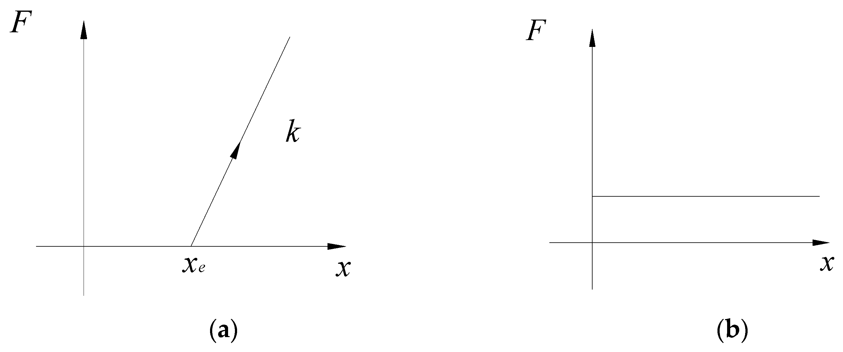
Because the engine block is very rigid compared with other parts of the vehicle and the pier, the contact process can be simulated as a rigid body crashing into the bridge pier, which means an elastic spring between the engine and pier is considered. And the spring only comes into effect after the engine surface has crashed into the bridge pier surface. The force–displacement of k1 and k2 is represented in Figure 5a, where xe is the distance from the engine to the head of the vehicle or the distance from the cargo mass to the head of the vehicle. During the finite element analysis (FEA), it was observed that the secondary impact load resulting from the cargo mass either did not occur or was significantly lower than the primary impact load generated by the engine. This behavior is attributed to the vehicle’s deceleration during the primary impact at lower speeds, which prevents the cargo from developing sufficient momentum for a subsequent collision. At higher speeds, the full failure of the pier typically occurs during the first impact, rendering any secondary impact effect negligible. Therefore, this study will focus on the primary rigid impact between the engine and the pier. The secondary impact by cargo mass with the spring stiffness k2 will be ignored here.
The damping force induced by c1 and c2 will be simplified into the constant damping force as a friction damper only if there is relative movement and compression between two parts, as shown in Figure 5b.

3.3. Tractor–Trailer

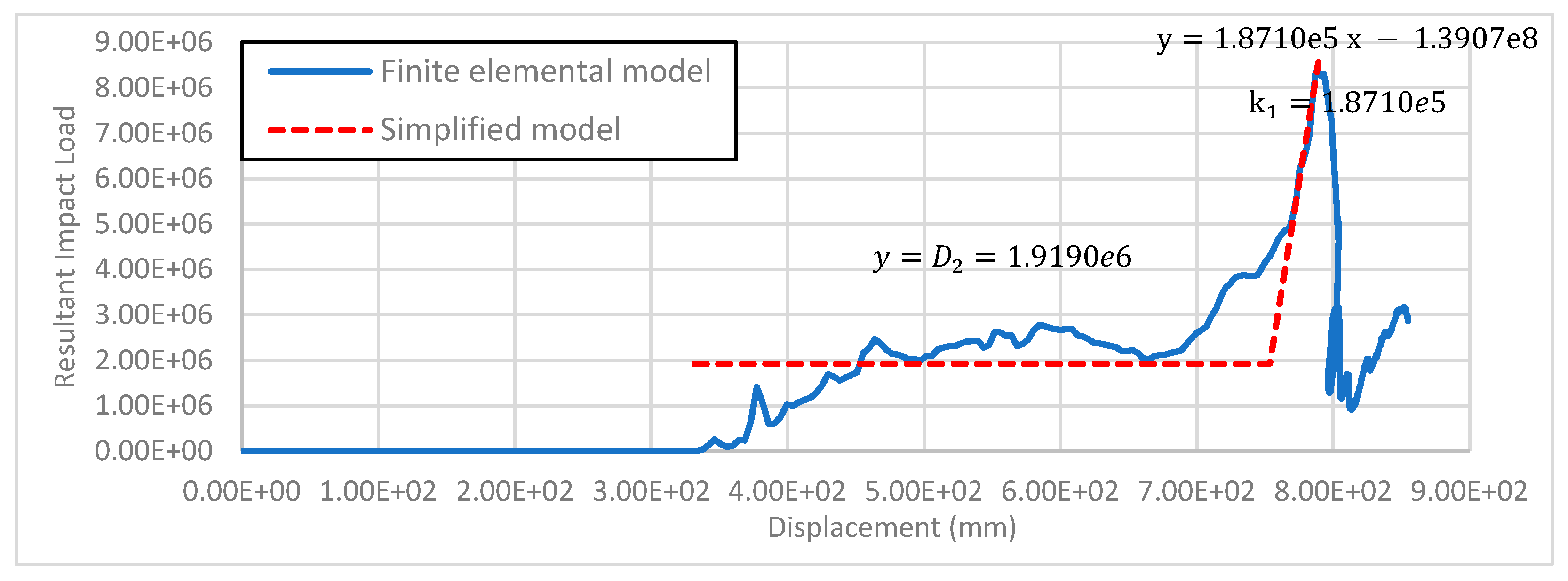
By examining the finite element analysis (FEA) results, it was observed that before the engine block (rigid body) collides with the pier, the front vehicle components undergo progressive crushing and absorb a significant portion of the impact energy. During this initial deformation stage, the impact force remains approximately constant compared with the sharp peak that occurs once the rigid body makes contact with the pier. Consequently, the constant damping force in the simplified model is assumed to represent the equivalent static load corresponding to the vehicle body’s plastic deformation prior to rigid-body impact. In this formulation, the constant damping force generated by c2 is considered equivalent to the static load component associated with the energy absorbed through vehicle deformation.
D 2 = 1.9190 × 10 6   N
During the engine collision phase, the impact load–displacement curve exhibits an approximately linear relationship up to the peak impact load, indicating an elastic interaction between the rigid body and the pier. Accordingly, the spring stiffness (k1) can be determined from the linear regression of the load–displacement response obtained for the engine component, ensuring that the simplified model accurately reflects the elastic stiffness of the pier during rigid-body impact, as shown in Figure 6.
Based on the linear regression function of the impact–displacement diagram, the following can be obtained:
x e = D 2 + 1.3907 e 8 k 1 332 = 422   m m
Before the engine block impacts the pier, it experiences deceleration caused by the crushing interaction between the engine and the previously yielded vehicle components around the engine. The constant damping force associated with c1 is therefore derived using the theorem of momentum, which relates the impulse generated during this deceleration phase to the change in momentum of the engine:
D 1 = M e v t = 3.53 × 10 5   N
where M e is the dry mass of the engine with 1.287 ton; v = 0.625 × 10 4   m m ; t = 0.0228   s

3.4. Pier Model

To perform the analysis of the pier, the pier is also transformed into a linear SDOF mass–spring system based on the Rayleigh–Ritz method according to Chopra [24]:
M P = m ¯ φ ( y ) 2 d x
where M P is the equivalent mass of the pier; m ¯ is the mass per unit length of the pier; φ ( y ) is assumed as the static deflection shape divided by the deflection at the nominal impact height under unit load.
For the pier fixed at one end, based on linear elastic theory, the relation between the deflection and curvature at the impact height can be given as follows:
E I ϕ I = M I
δ I = P I L I 3 3 E I = M I L I 2 3 E I
ϕ I = 3 L I 2 δ I
where ϕ I is the curvature of the beam at the impact height; δ I is the deflection at the impact height; M I is the moment at the impact height; L I is the impact height.
(A)
Concrete model
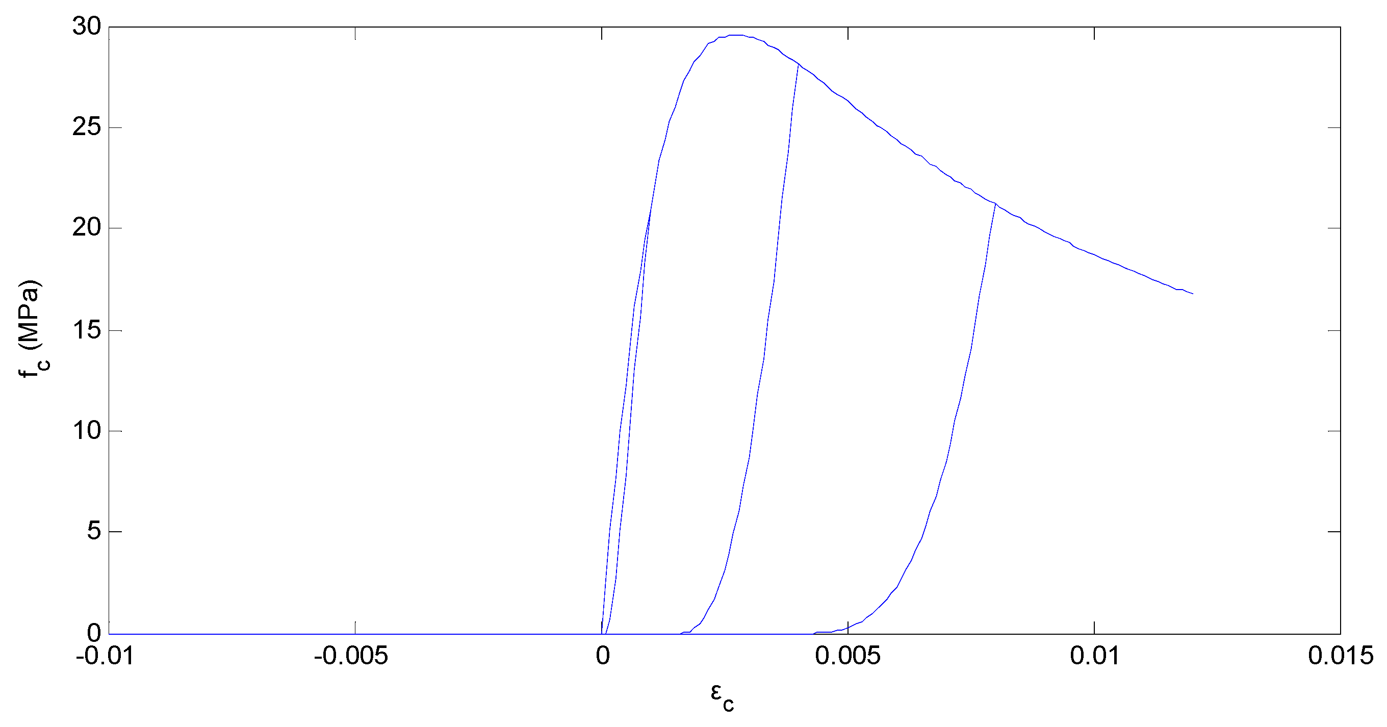
Based on the Mander model [25], the stress–strain relationship of concrete could be calculated for concrete with a strength of 27.58 MPa (4000 psi), which represents the most commonly used concrete strength for bridge piers in Department of Transportation (DOT) projects across the United States, as shown in Figure 7.
(B)
Steel model
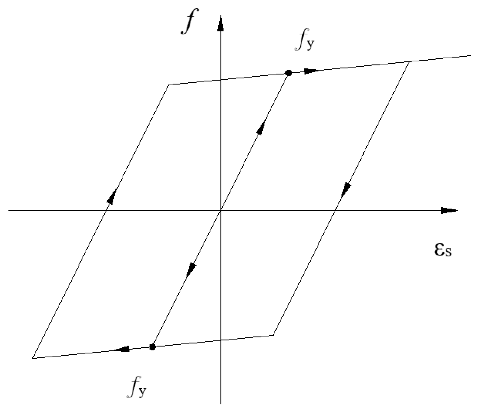
Steel uses a bilinear model. The unloading stiffness is equal to the steel stiffness. The stress–strain relationship of the steel reinforcement is shown in Figure 8.
(C)
Fiber model of pier section for analytical moment–curvature relationship
The section of the concrete pier is divided into n-fiber concrete elements and m-fiber reinforcement elements, as shown in Figure 9. The axial load and bending moment acting on the section at any curvature ϕ can be obtained as follows [26]:
N = A f d A = i = 1 n f c i A c i + J = 1 M f s j A s j
M = A f y d A = i = 1 n f c i y c i A c i + J = 1 M f s i y s j A s j
where y is the distance from the element to the neutral axis.
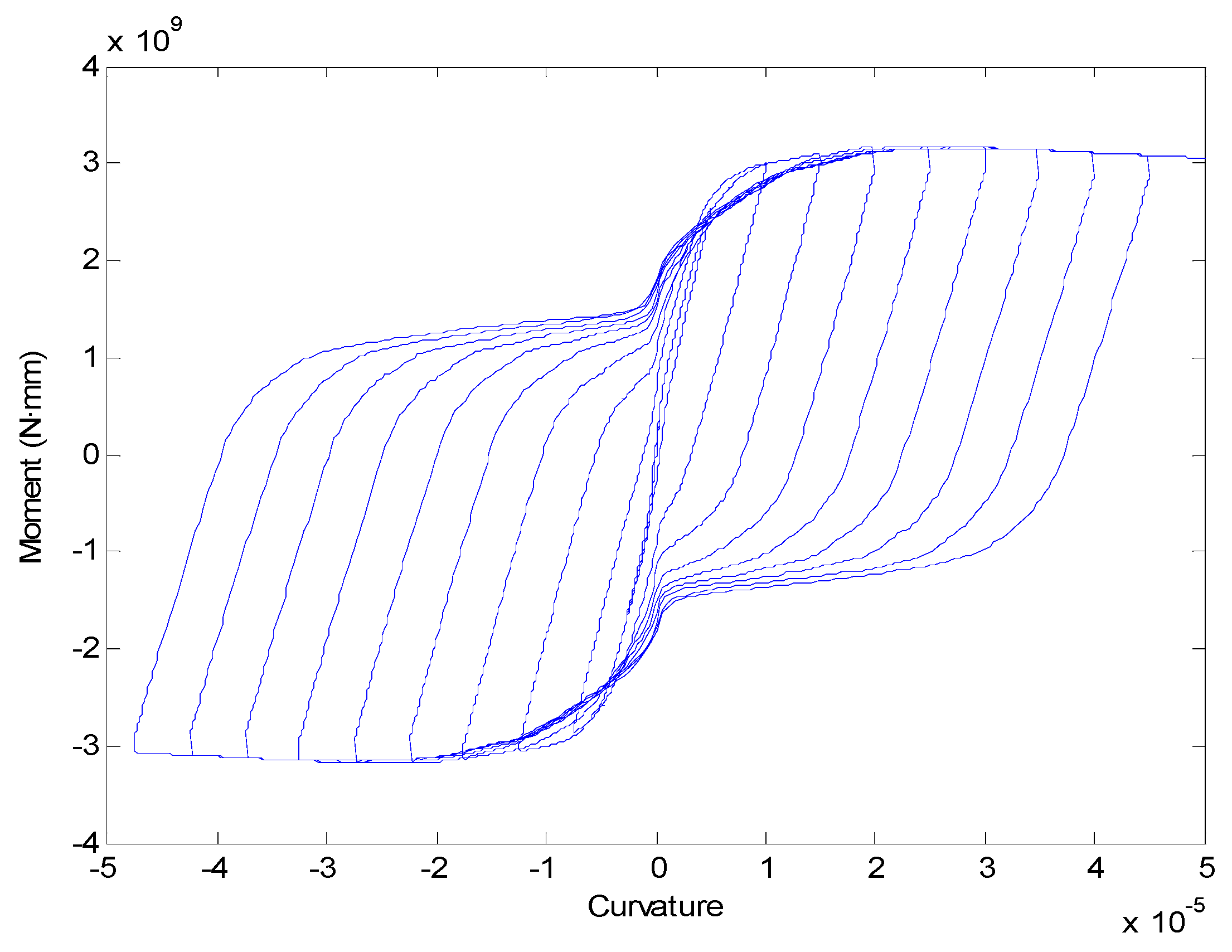
Due to the nonlinear variation in stress in the concrete element, the neutral axis will shift up and down during dynamic variation. In each step of analysis, Equation (11) will first be calculated based on the initial axial load to find the location of the neutral axis with several trials. Then, based on Equation (12), the moment corresponding to a specific curvature can be found. We take the strain rate of 104 s−1, which is a common value for impact loading based on Sierakowsi, S.K. Chaturved [27]. The dynamic increase factor of steel reinforcement is 1.3, while the dynamic increase factor of concrete is 1.5. The moment–curvature relationship of the pier under cyclic load is plotted in Figure 10. Finally, based on Equation (12), the relationship between the moment and the deflection at the nominal impact height can be obtained.

3.5. Explicit Dynamic Analysis for Coupling System

An explicit dynamic analysis is conducted based on the central difference method. The impact load in the 0.1 s after the initial contact between the truck and the pier will be considered. The time step takes t = 10−5 s, and there are a total of 10,000 steps.
At the nth time step,
u _ n = u e n u P n
u ˙ _ n = u _ n 1 + u _ n + 1 2 t         u ¨ _ n = u _ n 1 2 u _ n + u _ n + 1 t 2      
Given the initial condition at t = 0 and t = t ,
u _ 0 = 0 0 ; u _ 1 = v t 0
The mass matrix can be written as follows:
M = M e M P                  
Assume that the constant damping force is equal to D1 and D2 for the assumed dampers c1 and c2; the equation of motion can be changed to the following:
M u _ n 1 2 u _ n + u _ n + 1 t 2 + D + f s n = 0  
D = D 1 D 2
f s n = f e f P  
The force in the assumed spring k 1 is as follows:
f e = k 1 u e n u P n x e         u e n u P n x e > 0 0                                         u e n u P n x e < 0
The force acting on the pier due to the spring k 1 and its own resistance based on the moment–curvature relationship is as follows:
f P = f e + M ( u P n ) / L I
where M ( u P n ) is the moment when the deflection is equal to u P n at the impact height; L I is the nominal impact height.
Transferring the known quantities to the right side, the following is obtained:
K t * u _ n + 1 = P _ n *  
K t * = M t 2  
P _ n * = D M t 2 u _ n 1 f s n + 2 M t 2 u _ n    
u _ n + 1 = K t * 1 P _ n *  

3.6. Analyzed Results

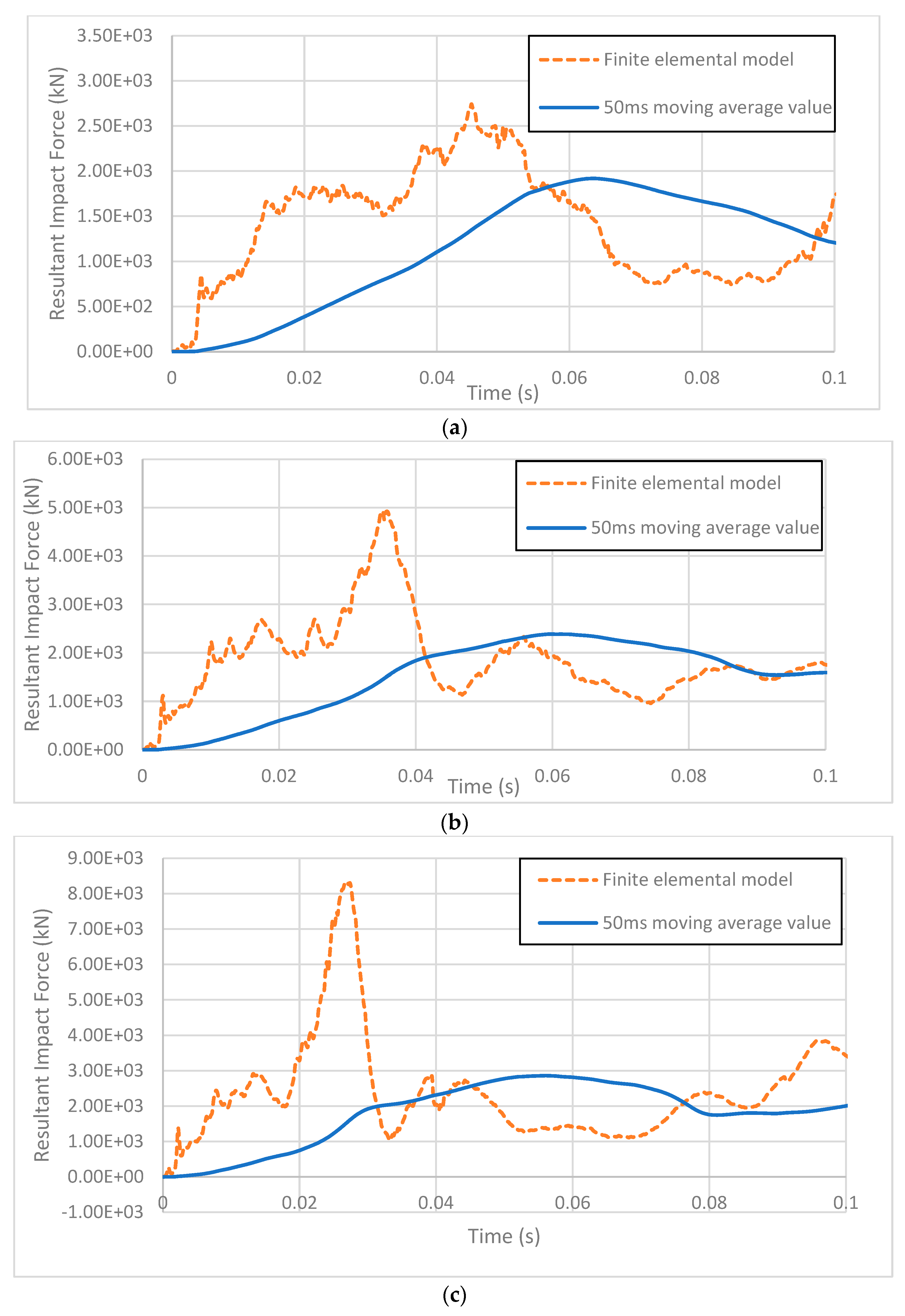
To verify the feasibility of the simplified model, the peak dynamic results and the equivalent static results, which are taken as the maximum 50 ms moving average value, are compared with the finite element analytical results of the tractor–trailer truck crashing into the pier with initial speeds of 60 km/h, 80 km/h, 100 km/h, and 120 km/h in accordance with the previous assumption, as shown in Figure 11.
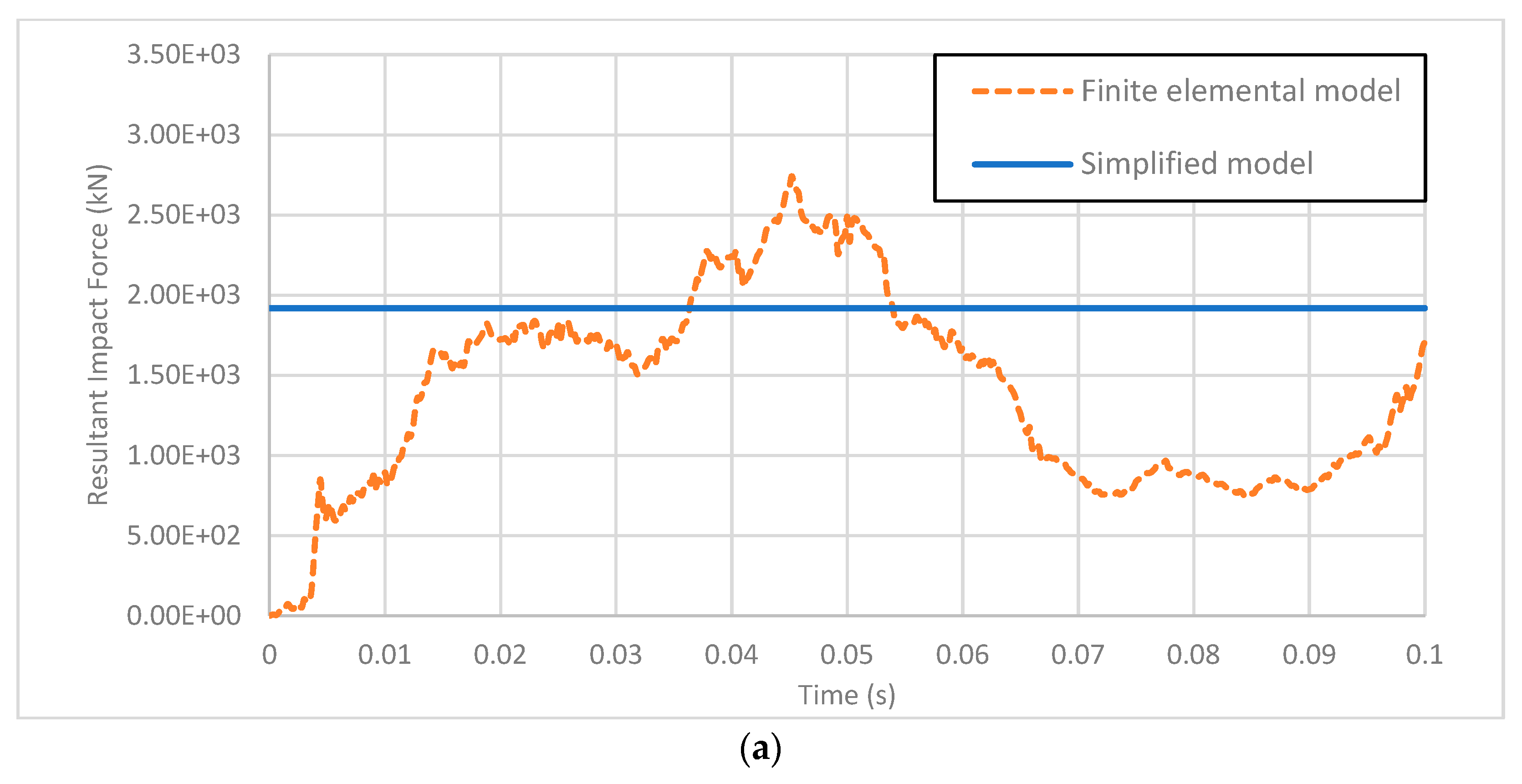
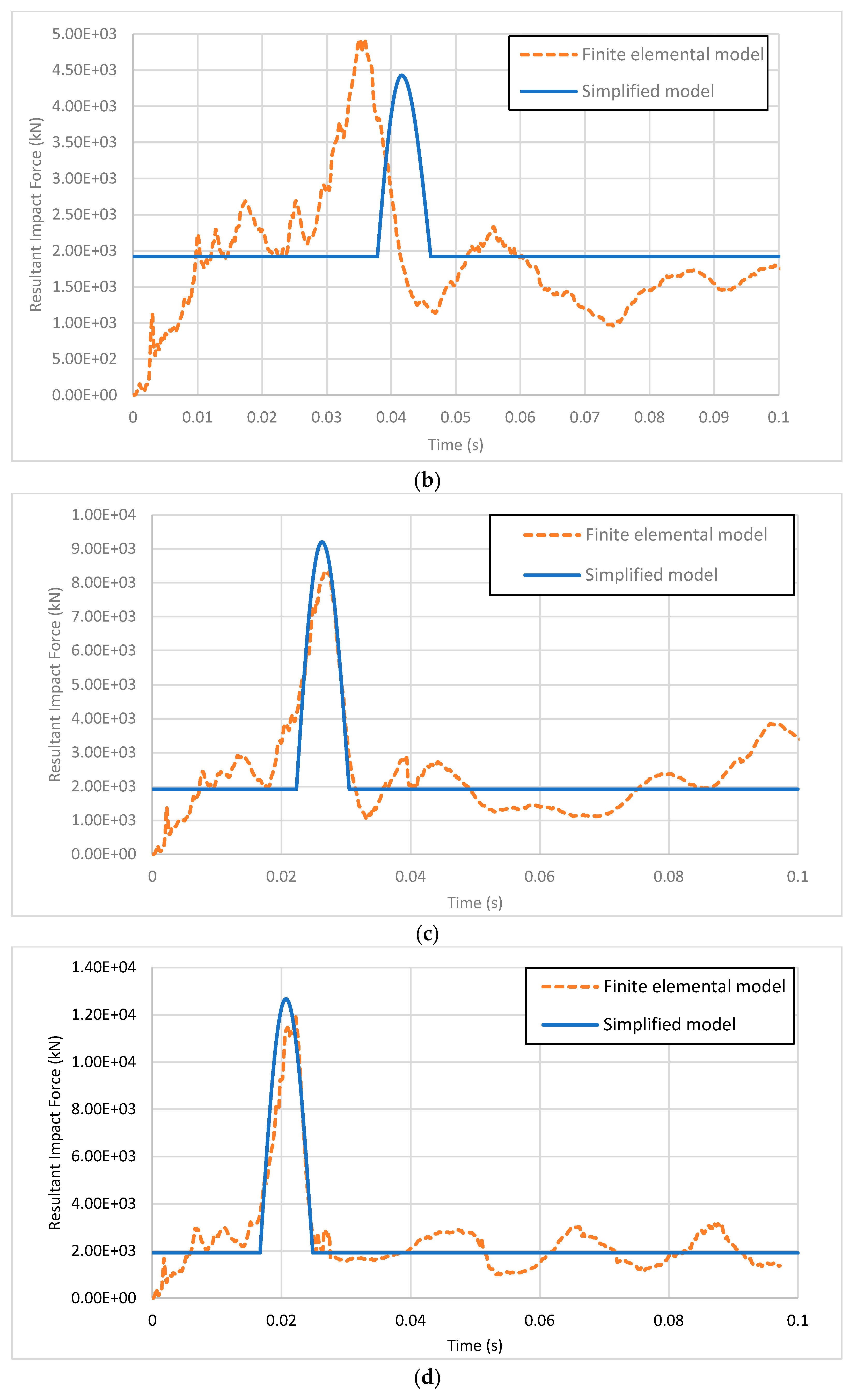
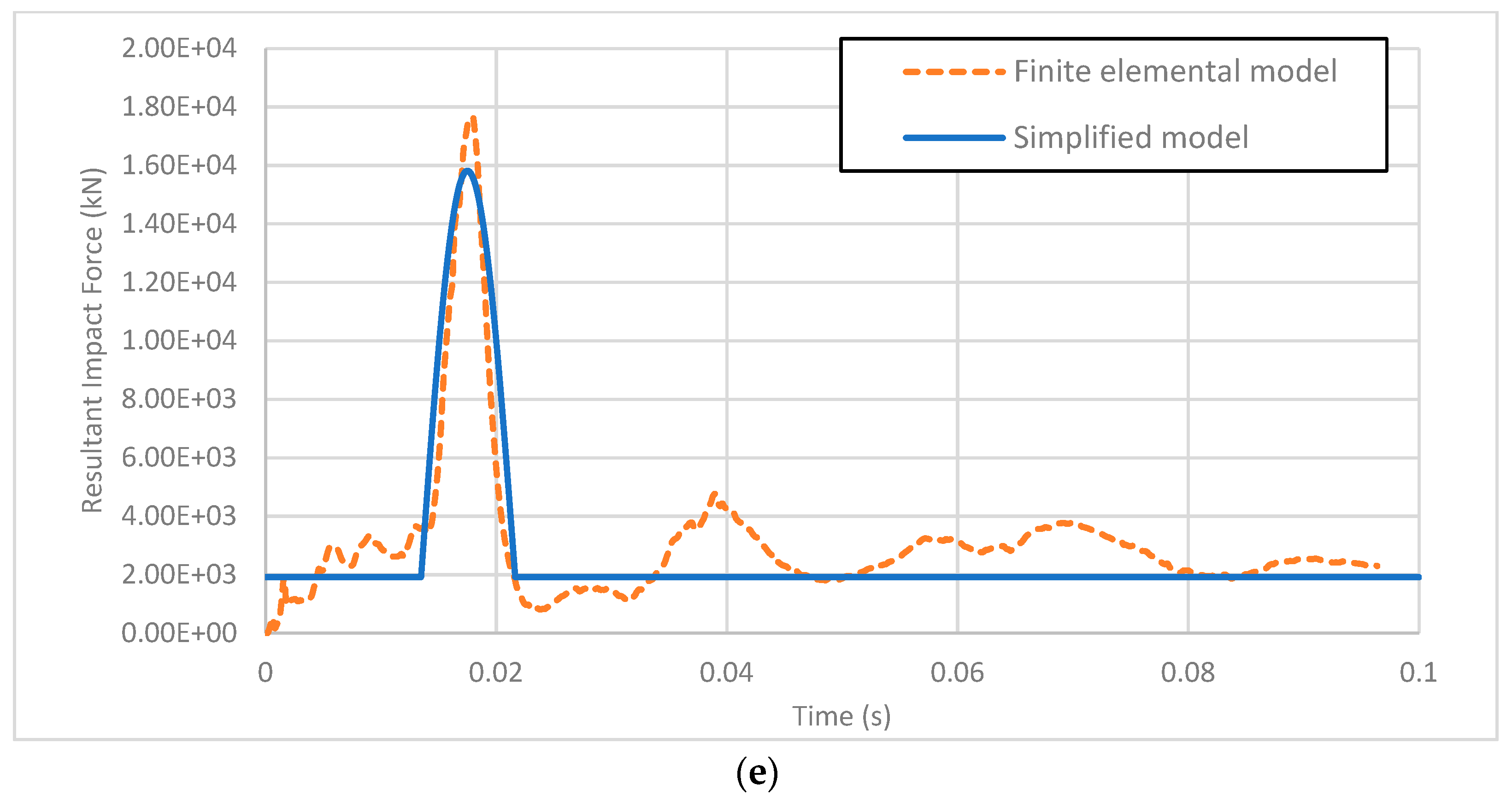
As shown in Figure 12, the results based on an explicit dynamic analysis of the simplified model show good fits with the finite element results. For the truck at a speed of 40 km/h, the analytical result has no rigid impact load induced between the engine and the pier. The curve shows a constant damping force induced by the crushing of the soft parts of the truck. For the truck at an initial velocity over 40 km/h, the analytical result shows an obvious peak dynamic impact load above the constant damping force. For the truck speed of 60 km/h, the peak impact load of the simplified model happens later than that of the finite element model. However, the value of the peak impact load matches well with the finite element model. For the truck at an impact speed over 60 km/h, the corresponding time of the peak impact load matches well with the finite element result. The peak dynamic values of the simplified model at 80 km/h and 100 km/h are slightly larger than the peak dynamic value of the finite element model. The peak dynamic value of the simplified model at 120 km/h is slightly smaller than that of the finite element model. Based on Table 1, the equivalent static force of the simplified model also shows good consistence with the finite element result.
The relatively large error (approximately 30%) observed under the low-speed impact condition (40 km/h) results from the simplified modeling assumption that all vehicle components, except for the stiff cargo and engine, are represented by constant damping elements. At such low velocities, the truck may come to a stop before the engine block actually contacts the pier, and several vehicle components undergo only partial deformation without being fully crushed. Representing these components solely as damping elements consequently underestimates their effective stiffness contribution, leading to deviations in the predicted peak dynamic load. A more accurate simulation within this low-speed range would involve modeling the undamaged components as additional mass–spring nodes to better capture their elastic behavior. Another limitation of the simplified model described above is that the shear mechanism is not included in the stiffness matrix. When shear failure governs the pier’s overall response, the model may therefore fail to accurately represent its true dynamic behavior. To address this limitation, shear deformation could be incorporated into the governing equations presented in Section 3.5; however, doing so would substantially increase the computational complexity and the difficulty of solving large-scale dynamic systems.
(2)
Impact Load Model Based on Response Surface Method

3.7. Overview

As we can see in the previous section, the simplified model based on the dynamic method can reflect the impact load to some extent, but there is limitation in accuracy based on the assumed dynamic system. In addition, a case-by-case analysis based on an explicit dynamic method is still required to obtain the impact load. For the requirement of small time steps in analysis, computer-aided computation is inevitable during analysis. To move forward in obtaining the impact load with a simple formula when the corresponding parameters are known, the response surface method is a good tool.
The reduced-order dynamic model idealizes the vehicle–pier interaction through a lumped mass system with equivalent spring and damping elements. This reduced-order approach retains the essential dynamic behavior of the coupled system while greatly simplifying computation, allowing engineers to obtain the time history of the impact force without performing full finite element simulations. In contrast, the response surface model is a purely statistical or regression-based method derived from a large number of finite element simulations. While the reduced-order dynamic model focuses on reproducing the physical impact process and temporal response, the response surface model provides a convenient algebraic expression for predicting peak impact loads or equivalent static loads without the need for dynamic analysis.
The response surface method was first introduced by Box and Wilson in 1951 [28]. It is a method based on empirical models, which is based on existing data to predict an unknown but desirable target. The response surface model is based on the Tylor approximation of a function with multiple variables. Taking the second-order Tylor expansion as an example, for an arbitrary function with n variables, x 1   t o   x n , we can approximate the accurate value of the function by the second-order polynomial:
f x 1 , , x n f x ~ 1 , , x ~ n + p = 1 n f x p x ~ 1 , , x ~ n x p x ~ p + 1 2 ! p = 1 n q = 1 n f x p x q x ~ 1 , , x ~ n x p x ~ p x q x ~ q + ϵ            
where x ~ 1 , , x ~ n is a fixed point, and ϵ represents the higher-order smaller quantities of x ~ 1 , , x ~ n .   ϵ can be ignored if the distances | x p x ~ p | are all sufficiently small. This equation can be expressed approximately after ignoring the higher-order smaller quantities ϵ as follows:
f R S x 1 , , x n = C 0 + C 1 x 1 + + C n x n + C 11 x 1 2 + C 12 x 1 x 2 + + C n 1 , n x n 1 x n + C n , n x n 2
ϵ = f x 1 , , x n f R S x 1 , , x n
For a load model of which the closed form is difficult to obtain, with at least ( n 2 + 3 n + 2 ) / 2 known groups of ( f x 1 , , x n , x 1 ,…,   x n ), the factors C 0 , , C n , n can be obtained. And in this way, the approximate formulation for f x 1 , , x n with second-order variables can be obtained. In the matrix equation, Equation (29) can be expressed as follows:
f x 1 , , x n 1 f x 1 , , x n i f x 1 , , x n N = 1 x 1 1 x n 1 x 1 2 1 x 1 x 2 1 x n 2 1 1 x 1 i x n i x 1 2 i x 1 x 2 i x n 2 i 1 x 1 N x n N x 1 2 N x 1 x 2 N x n 2 N C 0 C 1 C n C 11 C 12 C n , n + ϵ 1 ϵ i ϵ N Y = X C + ϵ
where ( 1 , x 1 i , , x n i , x 1 2 i ,   x 1 x 2 i ,     ,   x n 2 i   ) is the ith group of variables, and N > ( n 2 + 3 n + 2 ) / 2 ; Y is the response vector, also called the vector of observed values; X is the matrix of variables; C is the vector of parameters; ϵ is the error vector.
Based on linear regression, with N groups of variables, the parameter vector is obtained with the least-squares estimation method. The approximation response function for Equation (27) can be obtained.
To design N groups of variables, statistical criteria are used to minimize the variance of estimators. The D-optimal design method will be used in the design in this section. D-optimal design can be used for a limited number of designs and can save more computational effort compared with the standard method. In the multiple regression setting, the matrix X is often used to represent the data matrix of independent variables. D-optimality minimizes the overall variance of the estimated regression coefficients by maximizing the determinant of matrix X X or equivalently minimizing the value of the determinant of matrix ( X X ) 1 .
According to the results of this study, the impact loads are not equally sensitive to all parameters. Due to the high computation resource consumption required during the analysis for each case, the following sensitive parameters are included here: the impact velocity of the truck, the concrete strength, the diameter of the pier, the length of the pier, the height of the impact location, the axial stress on the pier, and the mass of the cargo. The number of parameters is seven, which requires at least 36 groups of parameters for the design. Five groups of Lack-of-fit points and five groups of replicate randomly generated points are added to the model to increase the robustness of the estimation. In addition, parameter groups are also added to the design as Lack-of-fit points to increase robustness.
To check accuracy, R-square and the root-mean-square error (RMSE) are used:
R 2 = 1 i = 1 N f R S i f i i = 1 N f i f ¯
R M S E = 1 N f ¯ i = 1 N f R S i f i 2
where f R S i is the impact load obtained based on the response surface model corresponding to the ith group of variables; f i is the impact load from FEM corresponding to the ith group of variables; N is the total N groups of variables, that is, N design points.
Cook’s distance is also included to measure the influence of each set of parameters on the response surface model [29]. Cook’s distance for the estimation of the ith group of parameters is calculated as follows:
D i = r i 2 p + 1 L e v e r a g e i 1 L e v e r a g e i
H = X ( X X ) 1 X
L e v e r a g e i = i t h   d i a g o n a l   e l e m e n t   o f   H
r i = ϵ i σ ^ 1 L e v e r a g e i
σ ^ 2 = i = 1 N ϵ i 2 n p 1
ϵ i = f i f R S i
where p is the number of terms in the model.
Cook’s distance can be thought of as the average squared difference between the predictions that result from the full dataset and those that result from a reduced dataset (deleting the ith observation) compared to the error mean squared of the fitted model. An equivalent interpretation of D i is a standardized weighted distance between the vector of regression coefficients obtained from the full model and the vector obtained after deleting the ith case. If the value of D i is substantially less than 1, deleting the ith case will not change the estimates of the regression coefficients very much. If the value of D i is larger than 1, it means that by deleting the ith case, the regression function of the response surface model will change obviously. This means that the data on the ith case is abnormal, which needs to be excluded during the regression analysis.

3.8. Response Surface Model

For tractor–trailer trucks,
f R S A , B , C , D , E , F , G = γ 0 + γ 1 A + γ 2 B + γ 3 C + γ 4 D + γ 5 E + γ 6 F + γ 7 G + γ 8 A B + γ 9 A C + γ 10 A D + γ 11 A E + γ 12 A F + γ 13 A G + γ 14 B C + γ 15 B D + γ 16 B E + γ 17 B F + γ 18 B G + γ 19 C D + γ 20 C E + γ 21 C F + γ 22 C G + γ 23 D E + γ 24 D F + γ 25 D G + γ 26 E F + γ 27 E G + γ 28 F G + γ 29 A 2 + γ 30 B 2 + γ 31 C 2 + γ 32 D 2 + γ 33 E 2 + γ 34 F 2 + γ 35 G 2
Table 2 shows the seven variables and their ranges for the regression analysis. The design points are discretely distributed at their design levels. Equation (38) is the quadratic response surface model for tractor–trailer trucks. A total of 36 factors γ 0 ,   γ 1 ,   ,   γ 35 are included in Equation (38). To determine the value for the 36 factors, 36 cases with different parameter sets, five (5) Lack-of-fit points, and five (5) replicated design points are generated based on the D-optimal method. In addition, 17 are added to increase the sample size and robustness. Therefore, a total of 63 finite element cases with different groups of parameters and responses are included in the analysis for tractor–trailer trucks. The parameters and responses of 63 finite element cases are shown in Table A1 Appendix A.
The values of the 36 factors are obtained by linear regression, as shown in Table A2 Appendix A. The coded value of the coefficient is used to normalize the range of variables from −1 to 1, where the minimum value corresponds to −1, the medium value corresponds to 0, and the maximum value corresponds to 1. For the coded equation, γ 1 is much larger than other factors, which means that the response is the most sensitive to the change in velocity.
The diagnostics based on Cook’s distance and an analysis of variance (ANOVA) are shown in Table 3 and Table 4 for peak dynamic impact load and equivalent static impact load. Cook’s distances for all cases are smaller than 1. The values of R2 are all close to 1.0, and the values of the RMSE are close to 0, which indicates that the response surface model provides a good fit.
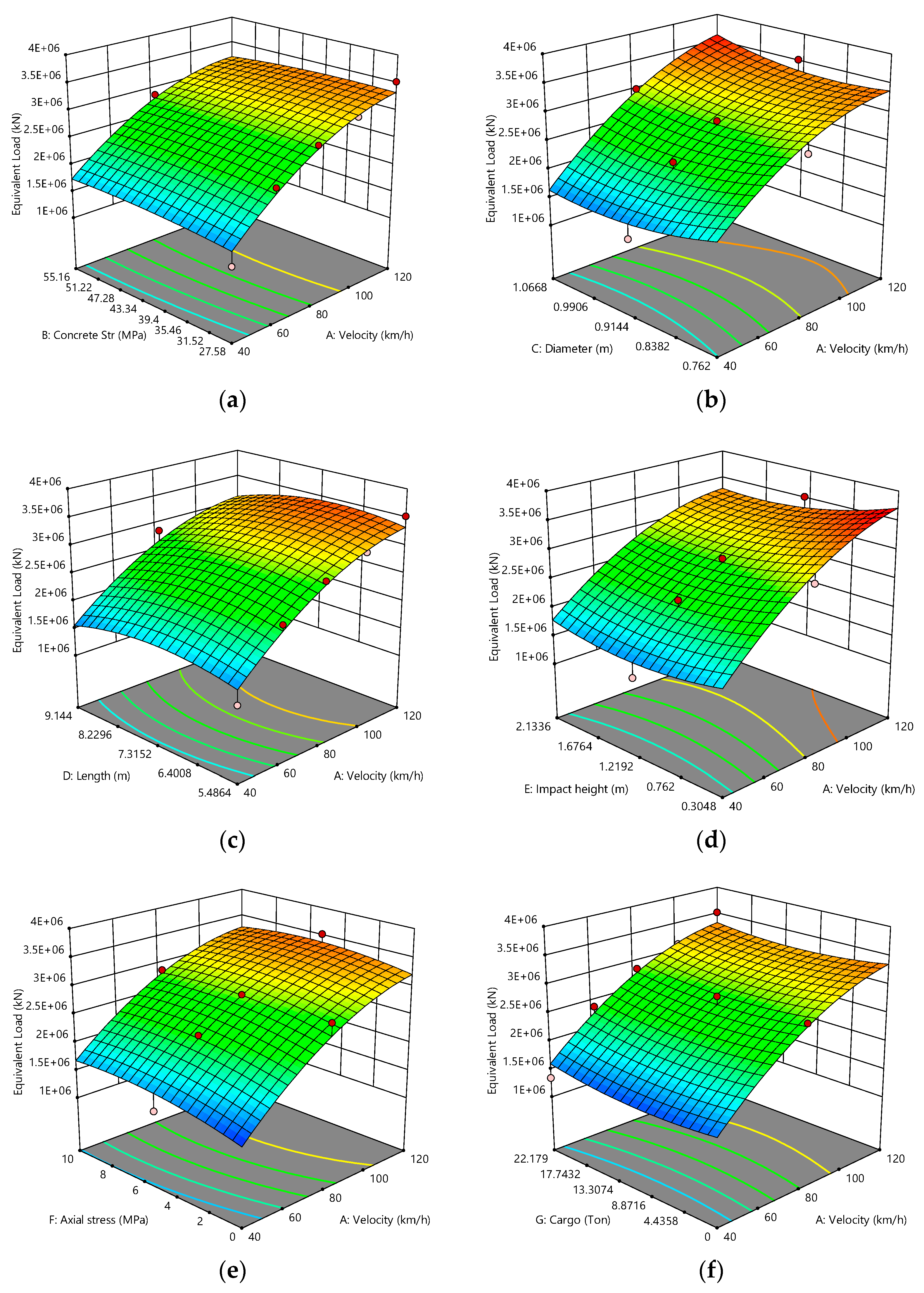
A 3D plot of the response surface model is shown in Figure A1 and Figure A2 of Appendix B based on the basic group of parameters A = 100 km/h, B = 27.58 MPa, C = 0.9144 m, D = 5.4864 m, E = 1.2192 m, F = 5 MPa, and G = 22.179 ton. The 3D response surface plots presented in Appendix B illustrate how the predicted impact loads vary with key influencing parameters, including vehicle speed, cargo weight, and pier diameter. These plots show that the impact load increases the most sharply with vehicle speed, exhibiting a steeper slope along the axis of vehicle speed, which confirms that kinetic energy is the dominant factor governing collision severity. The smooth curvature of the fitted surfaces validates the accuracy of the second-order polynomial functions used in the response surface model and demonstrates that the proposed equation effectively captures the combined influence of these parameters on the resulting impact loads. The design points, shown as red dots, closely align with the response surfaces, indicating an excellent fit of the model to the simulation data. Moreover, the plots highlight that the model response is significantly more sensitive to vehicle speed compared with other parameters, reinforcing the importance of velocity in determining impact intensity.
Although the regression model achieved high R2 values, consideration was given to the potential risk of overfitting arising from the limited number of data points (63) relative to the total number of regression terms (36). The model’s predictive capability beyond the calibrated parameter space may therefore be constrained, and additional data enrichment or adaptive sampling would be required in future work to enhance its generalizability and verify its robustness.

4. Summary

This study shows that both the reduced-order dynamic model and the response surface model could be applied to the approximate impact force. The reduced-order dynamic model is suitable for obtaining the time history of the impact force. However, appropriate assumptions must be made for the spring stiffness and damper. In addition, it is very hard to include the shear failure in the simulation even though it is the most common failure mechanism during truck-to-pier impact. To finish the calculation of the explicit analysis, computer-aided computation is required. Also, for each different truck and pier, an individual case-by-case analysis is required.
Relatively, the response surface model can provide an approximation equation for impact load, which is convenient and easy to apply to different impact scenarios by varying the value of parameters only if the parameters have been included in the model in advance. However, the response surface model cannot be applied to time history, although it is good at obtaining the response of key indices. Another drawback is that a prerequisite database is needed for regression analysis. Sometimes, a large number of design points is required in order to increase the precision of the fitting function. If the response has large discreteness, the regression model may be trapped in finding better fit.

5. Conclusions

This study proposed and evaluated two simplified models to improve the estimation of vehicle-induced impact loads on bridge piers: a reduced-order dynamic model and a response surface model.
(1)
Reduced-order dynamic model: This approach provides the time history response of impact forces through an idealized mass–spring–damper system. Although it requires appropriate assumptions for stiffness and damping and case-by-case explicit analyses, it effectively captures the dynamic behavior of the pier, including plastic deformation modeled through fiber section analysis. The framework can be extended to simulate various truck-to-pier and ship-to-pier impact scenarios and is particularly suitable when time history responses are of interest.
(2)
Response surface model: This method offers a direct analytical function for estimating impact loads based on key parameters such as vehicle speed, cargo mass, and pier geometry. By employing second-order polynomial fitting, it can efficiently predict both peak dynamic and equivalent static impact loads. The model can be further refined using large datasets or advanced sensitivity analysis; however, it cannot reproduce detailed time history responses.
Overall, this study provides a comprehensive parametric investigation of impact loads and pier responses and introduces two practical tools that can estimate impact loads without the need for full-scale finite element simulations. Both models provide more realistic and flexible design values than the constant, conservative load specified in the AASHTO LRFD Bridge Design Specifications.

Author Contributions

The authors confirm their contributions to the paper as follows: study conception and design: C.C.F. and C.X.; data collection: C.X.; analysis and interpretation of results: C.X. and C.C.F.; draft manuscript preparation: C.X. and C.C.F. All authors have read and agreed to the published version of the manuscript.

Funding

The research for this paper was conducted as part of a BEST Center project (project No. MD-21-SHA-UM/5-28) for the Maryland State Highway Administration and partially supported by the USDOT. The dissertation writing was self-supported.

Data Availability Statement

Data are contained within the article.

Acknowledgments

We thank all those within the SHA who provided assistance in obtaining design and field data for this study. The main information of this study is from the Ph.D. thesis “Impact Load Model Analysis on the Vehicle-to-Pier Collision” by C. Xu, advised by C.C. Fu, University of Maryland, College Park, MD, USA, 2019.

Conflicts of Interest

The author(s) declared no potential conflicts of interest with respect to the research, authorship, and/or publication of this article.

Appendix A. Parameters Used in Response Surface Model

Table A1. Design layout for response surface model of tractor–trailer truck.
CaseVariablesResponses
ABCDEFGPeak Dynamic Load
(N)
Equivalent Static Load
(N)
14055.160.7629.1440.30481003.4619E+061.2285E+06
28041.370.7625.48641.21921011.08951.0121E+072.5005E+06
34055.160.7629.1442.1336022.1791.7149E+062.2995E+06
44027.581.06685.48640.30481002.7548E+061.7274E+06
54027.580.7629.1440.3048022.1791.9289E+061.3252E+06
68027.580.91445.48642.13361009.5244E+062.8214E+06
76027.581.06689.1441.21921006.8068E+062.3703E+06
84027.580.7625.48640.3048522.1792.1252E+062.0344E+06
94055.161.06689.1442.13361011.08952.8614E+061.6051E+06
104055.160.7625.48640.3048011.08952.1145E+062.0041E+06
1112027.580.91447.31520.3048511.08951.7659E+073.5847E+06
1210055.161.06685.48640.30481001.0190E+073.0335E+06
138041.370.7629.1441.2192508.6926E+062.5215E+06
1412027.581.06689.1440.3048002.0769E+073.6278E+06
154027.580.7625.48642.1336022.1791.9126E+061.9536E+06
164055.161.06685.48641.2192522.1792.4520E+061.7415E+06
174027.581.06685.48642.1336522.1792.6966E+061.8981E+06
188027.581.06685.48640.3048022.1791.0220E+072.8853E+06
1910041.371.06689.1442.1336522.1791.1900E+073.4272E+06
208027.581.06685.48640.3048022.1791.0220E+072.8853E+06
214041.371.06689.1440.30481022.1792.4932E+061.9003E+06
2212041.371.06687.31522.13361001.7971E+073.5437E+06
234027.581.06689.1442.1336022.1792.3190E+061.5052E+06
2412027.580.7629.1440.30481001.4901E+072.4729E+06
2512055.160.7629.1442.13361022.1791.6006E+072.5510E+06
264027.580.7629.1442.1336002.7663E+061.3999E+06
2712027.580.7625.48642.1336522.1791.4304E+073.5092E+06
2812027.580.7629.1442.1336022.1791.4778E+072.7548E+06
298027.580.7627.31520.3048008.3097E+062.6637E+06
3010041.370.7629.1440.30481022.1791.0769E+073.2134E+06
3112055.161.06689.1441.2192022.1791.9481E+073.4803E+06
324027.580.7627.31522.13361022.1793.5317E+062.2011E+06
334055.161.06685.48642.1336002.1534E+061.8325E+06
348027.580.7627.31520.3048008.3097E+062.6637E+06
3512055.160.7629.1440.3048011.08951.6099E+073.2187E+06
3612027.581.06685.48642.1336001.5672E+073.5898E+06
3712055.161.06685.48642.1336022.1791.7877E+073.2495E+06
384055.161.06689.1440.3048002.9305E+061.9843E+06
3912055.160.7625.48642.1336501.6073E+073.2817E+06
4012027.580.91447.31520.3048511.08951.7659E+073.5847E+06
4112041.371.06687.31522.13361001.7971E+073.5437E+06
4212055.160.7625.48640.30481022.1791.6815E+073.3439E+06
4312055.160.91449.1442.1336001.5576E+073.5722E+06
4412041.370.91445.48640.3048001.6636E+073.5934E+06
4512027.581.06685.48641.21921022.1791.8760E+073.4939E+06
4612041.370.91445.48640.3048001.6636E+073.5934E+06
474027.580.91445.48641.2192522.1792.1601E+061.3423E+06
486027.580.91445.48641.2192522.1794.9249E+062.3863E+06
498027.580.91445.48641.2192522.1798.3425E+062.8580E+06
5010027.580.91445.48641.2192522.1791.1924E+073.1123E+06
5112027.580.91445.48641.2192522.1791.7635E+073.5218E+06
528041.370.91445.48641.2192522.1797.9537E+062.8298E+06
538055.160.91445.48641.2192522.1797.0132E+062.8663E+06
548027.580.7625.48641.2192522.1797.4634E+062.7753E+06
558027.581.06685.48641.2192522.1791.1108E+072.9915E+06
568027.580.91447.31521.2192522.1798.1201E+062.8389E+06
578027.580.91449.1441.2192522.1798.2502E+062.8461E+06
588027.580.91445.48640.3048522.1798.4439E+062.9086E+06
598027.580.91445.48642.1336522.1796.9615E+062.5847E+06
608027.580.91445.48641.2192022.1797.6976E+062.8485E+06
618027.580.91445.48641.21921022.1798.4141E+062.8627E+06
628027.580.91445.48641.2192506.8596E+062.8173E+06
638027.580.91445.48641.2192511.08958.3987E+062.8025E+06
Table A2. Factors for response surface model of tractor–trailer truck.
Peak Dynamic LoadEquivalent Static Load
FactorsCoded
( × 10 6   N )
Actual
( × 10 6   N )
Coded
( × 10 5   N )
Actual
( × 10 5   N )
γ 0 8.8893894.17492329.181796.002955
γ 1 6.865914−0.111187.8831430.509356
γ 2 −0.189920.4224330.466960.660195
γ 3 0.417361−38.5870.975437−103.369
γ 4 −0.046772.084407−0.531815.842994
γ 5 0.005493.298193−0.275072.227506
γ 6 0.1340670.533173−1.047370.820623
γ 7 −0.06459−0.122580.5698890.289221
γ 8 0.0032245.85E−06−0.63602−0.00115
γ 9 0.6329720.1038341.0732080.176051
γ 10 0.0999990.001367−0.3731−0.0051
γ 11 −0.43816−0.01198−1.01407−0.02772
γ 12 −0.35636−0.00178−0.59336−0.00297
γ 13 0.5747750.001296−0.28269−0.00064
γ 14 −0.47741−0.22717−0.7044−0.33517
γ 15 −0.11736−0.004650.5527150.021916
γ 16 0.3963270.031431−0.26954−0.02138
γ 17 0.0731250.001061−1.54085−0.02235
γ 18 −0.04174−0.000270.0238750.000156
γ 19 0.2513630.9018841.0488983.763416
γ 20 −0.23306−1.6724−0.4007−2.87539
γ 21 −0.3373−0.442660.4709220.618008
γ 22 0.3001360.177591−0.82898−0.49051
γ 23 −0.22258−0.13310.1947110.116436
γ 24 −0.34645−0.037890.0856230.009364
γ 25 −0.21603−0.010650.1619480.007985
γ 26 0.5544410.121269−0.31117−0.06806
γ 27 −0.23899−0.02357−0.68908−0.06796
γ 28 −0.16175−0.002920.5436710.009805
γ 29 1.8678850.001167−3.32544−0.00208
γ 30 −0.54128−0.00285−0.57887−0.00304
γ 31 0.48389720.834511.11602648.05121
γ 32 −0.54445−0.16279−2.36625−0.7075
γ 33 −0.50619−0.60541.1814141.41296
γ 34 0.3968270.015873−1.31902−0.05276
γ 35 −0.09293−0.000761.2787420.010398

Appendix B. Three-Dimensional Response Surface Plots of Tractor–Trailer Truck
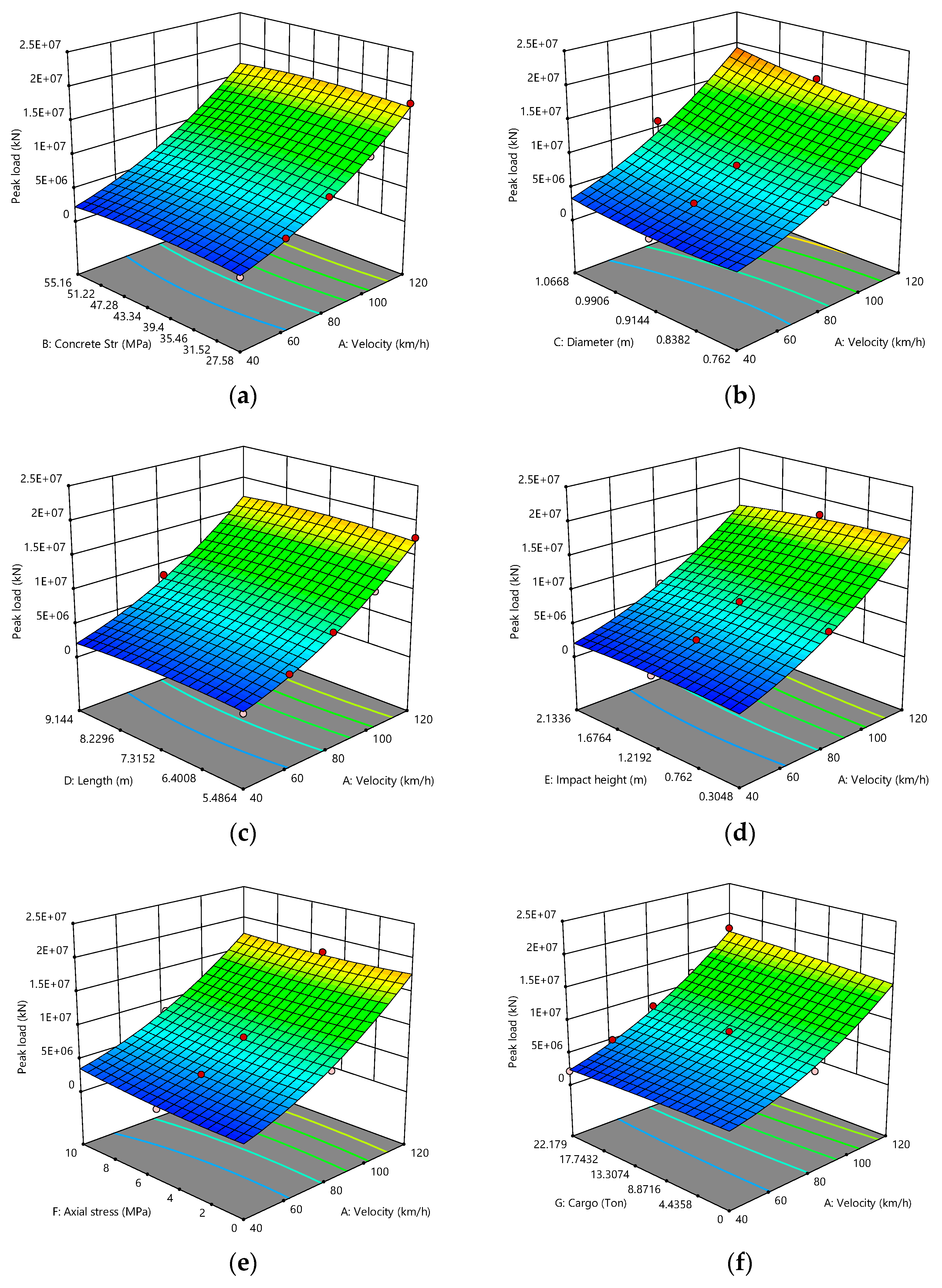
Figure A1. Three-dimensional response surface plot of peak dynamic load of tractor–trailer truck. (Basic parameters: A = 100 km/h; B = 27.58 MPa; C = 0.9144 m; D = 5.4864 m; E = 1.2192 m; F = 5 Mpa; G = 22.179 ton.) (a) A:B; (b) A:C; (c) A:D; (d) A:E; (e) A:F; (f) A:G.
Infrastructures 10 00320 g0a1
Figure A2. Three-dimensional response surface plot of equivalent static load of tractor–trailer truck. (Basic parameters: A = 100 km/h; B = 27.58 MPa; C = 0.9144 m; D = 5.4864 m; E = 1.2192 m; F = 5 MPa; G = 22.179 ton.) (a) A:B; (b) A:C; (c) A:D; (d) A:E; (e) A:F; (f) A:G.
Infrastructures 10 00320 g0a2

Appendix C. European Code

References

  1. Fu, C.C.; Burhouse, J.R.; Chang, G.L. Overheight vehicle collisions with highway bridges. Transport. Res. Rec. 2004, 1865, 80–88. [Google Scholar] [CrossRef]
  2. AASHTO. Load Resistance and Factor Design: Bridge Design Specifications, 9th ed.; American Association of State Highway and Transportation Officials: Washington, DC, USA, 2020. [Google Scholar]
  3. Buth, C.E.; Michael, S.B.; William, F.W.; Gary, T.F. Collision Loads on Bridge Piers: Phase 2, Report of Guidelines for Designing Bridge Piers and Abutments for Vehicle Collisions; Report FHWA/TX-11/9-4973-2; Texas A&M University: College Station, TX, USA, 2011. [Google Scholar]
  4. ASCE7-10; Minimum Design Loads for Buildings and Other Structures. American Society of Civil Engineers: Reston, VA, USA, 2010.
  5. Final Draft prEN 1991-1-1; Eurocode 1: Actions on Structures–Part 1-1: General Actions–Densities, Self-Weight, Imposed Loads for Buildings. Comité Europeo de Normalización: Brussels, Belgium, 2001. Available online: https://gaprojekt.com/wp-content/uploads/2021/11/Eurocode-1-Actions-on-Structures.pdf (accessed on 12 September 2017).
  6. Final Project Team Draft (Stage 34), Draft prEN 1991-1-7; Eurocode 1: Actions on Structures–Part 1-7: General Actions–Accidental Actions. Comité Europeo de Normalización: Brussels, Belgium, 2003. Available online: https://www.phd.eng.br/wp-content/uploads/2015/12/en.1991.1.7.2006.pdf (accessed on 12 September 2017).
  7. Ferrer, B.; Ivorra, S.; Segovia, E.; Irles, R. Tridimensional Modelization of the Impact of a Vehicle against a Metallic Parking Column at a Low Speed. Eng. Struct. 2010, 32, 1986–1992. [Google Scholar] [CrossRef]
  8. Sherif, E.-T.; Edward, S.; Priscilla, F. Vehicle Collision with Bridge Pier; Report BC355_06; University of Michigan: Ann Arbor, MI, USA, 2004. [Google Scholar]
  9. NCAC. 1994 Chevy C2500 Pick-Up. Available online: https://www.ccsa.gmu.edu/capability/ (accessed on 24 February 2016).
  10. NCAC. F800 Single Unit Truck FEM Model for Crash Simulations with LS-DYNA. Available online: https://thyme.ornl.gov/FHWA/F800WebPage/downloads/downloads.html (accessed on 12 September 2017).
  11. Consolazio, G.R.; Cowan, D.R. Numerically Efficient Dynamic Analysis of Barge Collisions with Bridge Pier. J. Struct. Eng. 2005, 131, 1256–1266. [Google Scholar] [CrossRef]
  12. Buth, C.E.; William, F.W.; Michael, S.B.; Dominique Lord, S.R.G.; Akram, Y.A.-O. Analysis of Large Truck Collisions with Bridge Piers: Phase 1, Report of Guidelines for Designing Bridge Piers and Abutments for Vehicle Collisions; Report FHWA/TX-10/9-4973-1; Texas A&M University: College Station, TX, USA, 2010. [Google Scholar]
  13. Liu, G. Behavior of Bridge Piers During Vehicular Impacts. Ph.D. Dissertation, City University of New York, New York, NY, USA, 2012. [Google Scholar]
  14. Fujikake, K.; Bing, L.; Sam, S. Impact Response of Reinforced Concrete Beam and Its Analytical Evaluation. J. Struct. Eng. 2009, 135, 938–950. [Google Scholar] [CrossRef]
  15. Mohammed, T. Reinforced Concrete Structural Members Under Impact Loading. Ph.D. Dissertation, University of Toledo, Toledo, OH, USA, 2011. [Google Scholar]
  16. Gomez, N.L. Performance of Circular Reinforced Concrete Bridge Piers Subjected to Vehicular Collisions. Master’s Thesis, University of Massachusetts—Amherst, Amherst, MA, USA, 2014. [Google Scholar]
  17. Abdelkarim, O.I.; Mohamed, A.E. Performance of Hollow-core FRP–concrete–steel Bridge Columns Subjected to Vehicle Collision. Eng. Struct. 2016, 123, 517–531. [Google Scholar] [CrossRef]
  18. Chen, L.; Sherif, E.-T.; Yan, X. Reduced Models for Simulating Collisions between Trucks and Bridge Piers. J. Bridge Eng. 2016, 21, 04016020. Available online: https://ascelibrary.org/doi/10.1061/%28ASCE%29BE.1943-5592.0000810 (accessed on 12 September 2017). [CrossRef]
  19. Do, T.V.; Thong, M.P.; Hong, H. A Dynamic responses and failure modes of bridge columns under vehicle collision. Eng. Struct. 2018, 156, 243–259. [Google Scholar] [CrossRef]
  20. Alomari, Q.A.; Daniel, G.L. Advanced analysis of intact, fire-damaged, and CFRP retrofitted bridge pier columns under vehicle collisions: Empirical equivalent static force equation and framework. Eng. Struct. 2024, 314, 118250. [Google Scholar] [CrossRef]
  21. Xu, C. Impact Load Model Analysis on the Vehicle-to-Pier Collision. Ph.D. Thesis, University of Maryland, College Park, MD, USA, 2019. [Google Scholar]
  22. NCAC. FEM Models for Semitrailer Trucks. Available online: https://thyme.ornl.gov/fhwa/tractortrailer/download/download.cgi (accessed on 12 September 2017).
  23. Greimann, L.; Wolde-Tinsae, A.M. Design Model for Piles in Jointless Bridges. J. Struct. Eng. 1998, 114, 1354–1371. [Google Scholar] [CrossRef]
  24. Chopra, A.K. Dynamics of Structures: Theory and Applications to Earthquake Engineering, 2nd ed.; Prentice Hall: Upper Saddle River, NJ, USA, 2000. [Google Scholar]
  25. Mander, J.B.; Priestley, M.J.N.; Park, R. Theoretical Stress-Strain Model for Confined Concrete. J. Struct. Eng. 1988, 114, 1804–1826. [Google Scholar] [CrossRef]
  26. Cosenza, E.; Carmine, G.; Giuseppe, M. A simplified method for flexural capacity assessment of circular RC cross-sections. Eng. Struct. 2011, 33, 942–946. [Google Scholar] [CrossRef]
  27. Sierakowski, R.L.; Chaturvedi, S.K. Dynamic Loading and Characterization of Fiber-Reinforced Composite; Wiley: New York, NY, USA, 1997. [Google Scholar]
  28. Box, G.E.; Wilson, K.B. On the Experimental Attainment of Optimum Conditions. J. R. Stat. Soc. 1951, 13, 1–45. [Google Scholar] [CrossRef]
  29. Cook, R.D. Detection of Influential Observation in Linear Regression. Technometrics 1977, 19, 15–18. [Google Scholar] [CrossRef]
Figure 1. Finite element model of reinforcement concrete beam for pier modeling validation.
Infrastructures 10 00320 g001
Figure 2. Impact force and mid-span deflection for S1322 beam with drop height of 2.40 m.
Infrastructures 10 00320 g002
Figure 3. Finite element model. (a) Tractor, day cabin, with 45 ft semitrailer. (b) Pier model. (c) Impact analysis at different truck speeds (40 km/h, 80 km/h, 100 km/h from left to right).
Infrastructures 10 00320 g003aInfrastructures 10 00320 g003b
Figure 4. Reduced-order dynamic model.
Infrastructures 10 00320 g004
Figure 5. Assumption of spring and damping between vehicle and pier. (a) Spring model; (b) damping model.
Infrastructures 10 00320 g005
Figure 6. Resultant impact force with respect to different engine displacements of tractor–trailer truck.
Infrastructures 10 00320 g006
Figure 7. Stress–strain relationship for confined concrete.
Infrastructures 10 00320 g007
Figure 11. Finite element dynamic result and equivalent static result. (a) Initial truck velocity at 40 km/h; (b) initial truck velocity at 60 km/h; (c) initial truck velocity at 80 km/h; (d) initial truck velocity at 100 km/h; (e) initial truck velocity at 120 km/h.
Infrastructures 10 00320 g011aInfrastructures 10 00320 g011b
Figure 12. Comparison of finite element result with analytical result based on simplified impact model for tractor–trailer truck. (a) Initial truck velocity at 40 km/h; (b) initial truck velocity at 60 km/h; (c) initial truck velocity at 80 km/h; (d) initial truck velocity at 100 km/h; (e) initial truck velocity at 120 km/h.
Infrastructures 10 00320 g012aInfrastructures 10 00320 g012bInfrastructures 10 00320 g012c
Figure 8. Stress–strain relationship for steel reinforcement.
Infrastructures 10 00320 g008
Figure 9. Fiber element model for concrete section.
Infrastructures 10 00320 g009
Figure 10. Moment–curvature relationship of concrete section.
Infrastructures 10 00320 g010
Table 1. Comparison of peak dynamic load and equivalent static load (tractor–trailer).
Initial VelocityPeak Dynamic Load (kN)Equivalent Static Load (kN)AASHTO LRFD (kN)
Finite ElementSimplified ModelErrorFinite ElementSimplified ModelError
40 km/h2742.41919.030.02%1919.01919.00.00%2669
60 km/h4924.94427.310.10%2386.32182.08.56%
80 km/h8342.59198.910.27%2858.02675.96.38%
100 km/h11,923.712,670.46.26%3112.23036.12.45%
120 km/h17,634.715,814.410.32%3521.83362.44.53%
Table 2. Factors for regression analysis of tractor–trailer truck.
VariablesNameUnitsMinimumMaximumLevelL[1]L[2]L[3]L[4]L[5]
AVelocitykm/h40.00120.005406080100120
BConcrete StrengthMPa27.5855.16327.5841.3755.16
CDiameterm0.76201.0730.7620.91441.0668
DLengthm5.499.1435.48647.31529.144
EImpact heightm0.30482.1330.30481.21922.1336
FAxial stressMPa0.000010.0030510
GCargoTon0.000022.1793011.0922.179
Table 3. Diagnostics and ANOVA for response surface model of peak dynamic load of tractor–trailer truck.
Standard deviation6.264E+05
Mean value (N)9.660E+06
R 2 0.9949
RMSE0.00535
Table 4. Diagnostics and ANOVA for response surface model of equivalent static load of tractor–trailer truck.
Standard deviation1.548E+05
Mean value (N)2.705E+06
R 2 0.9779
RMSE0.00472
Disclaimer/Publisher’s Note: The statements, opinions and data contained in all publications are solely those of the individual author(s) and contributor(s) and not of MDPI and/or the editor(s). MDPI and/or the editor(s) disclaim responsibility for any injury to people or property resulting from any ideas, methods, instructions or products referred to in the content.