Article

Bayesian Optimized of CNN-M-LSTM for Thermal Comfort Prediction and Load Forecasting in Commercial Buildings

1
Swinburne University of Technology, Hawthorn, VIC 3122, Australia
2
La Trobe University, Bundoora, VIC 3083, Australia
3
New Horizon College of Engineering, Bengaluru 560103, India
4
Curtin University, Singapore Campus, Singapore 117684, Singapore
*
Author to whom correspondence should be addressed.
Designs 2025, 9(3), 69; https://doi.org/10.3390/designs9030069
Submission received: 2 May 2025 / Revised: 22 May 2025 / Accepted: 26 May 2025 / Published: 4 June 2025

Abstract

Heating, ventilation, and air conditioning (HVAC) systems account for 60% of the energy consumption in commercial buildings. Each year, millions of dollars are spent on electricity bills by commercial building operators. To address this energy consumption challenge, a predictive model named Bayesian optimisation Convolution Neural Network Multivariate Long Short-term Memory (BO CNN-M-LSTM) is introduced in this research. The proposed model is designed to perform load forecasting, optimizing energy usage in commercial buildings. The CNN block extracts local features, whereas the M-LSTM captures temporal dependencies. The hyperparameter fine tuning framework applied Bayesian optimization to enhance output prediction by modifying model properties with data characteristics. Moreover, to improve occupant well-being in commercial buildings, the thermal comfort adaptive model developed by de Dear and Brager was applied to ambient temperature in the preprocessing stage. As a result, across all four datasets, the BO CNN-M-LSTM consistently outperformed other models, achieving an 8% improvement in mean percentage absolute error (MAPE), 2% in normalized root mean square error (NRMSE), and 2% in R2 score.This indicates the consistent performance of BO CNN-M-LSTM under varying environmental factors, highlight the model robustness and adaptability. Hence, the BO CNN-M-LSTM model is a highly effective predictive load forecasting tool for commercial building HVAC systems.

1. Introduction

With the significant increase of energy consumption and the integration of loads into commercial buildings, energy saving scheme have become a critical direction for sustainable development. For instance, in 2022, commercial buildings made up 30% of global final energy consumption, of which 35% was in the form of electricity [1]. In a related finding, the U.S. Energy Information Administration’s 2018 Commercial Buildings Energy Consumption Survey (CBECS) [2,3] revealed that electricity constituted 60% of the U.S.’s energy use for commercial buildings, making it a primary energy source. Heating, ventilation, and air conditioning (HVAC) systems were the main users of this electricity, resulting in an annual expenditure of USD 119 billion, or 84% of total energy costs in commercial buildings. These figures highlight the considerable energy consumption and associated costs of HVAC systems, underscoring the pressing need for increased energy efficiency in the building sector. Therefore, the development and implementation of effective control strategies for HVAC systems is essential, as displayed in Figure 1.
The systematic review indicates that local HVAC controllers, such as process control or sequencing control, can be energy-efficient and cost-effective for specific subsystems. However, these controllers may face challenges in balancing energy efficiency, cost-effectiveness, and maintaining indoor thermal comfort. In contrast, supervisory control methods, such as machine learning and deep learning techniques, exhibit the capability to account for all characteristics, interactions among components, and their associated variables. In particular, the demand response (DR) strategies that incentivize shifts in energy consumption patterns [4] have demonstrated significant potential for improving energy management. Given the substantial energy use of HVAC systems, optimizing their electricity consumption is particularly valuable. For instance, adaptive HVAC control systems, powered by Model Predictive Control (MPC) method [5], can dynamically adjust operations in response to real-time conditions, thus reduce electricity consumption during peak demand periods. This capability not only enhances the efficiency of DR programs but also supports power grid stability [6]. In commercial buildings, many studies [7,8,9,10] had applied MPC method to control zone temperatures and building thermal mass. In a 2024 study, Wang et al. [10] highlights the pivotal role of MPC, emphasising that its hinges on the accurate forecasting of key variables, such as energy consumption, temperature, and occupancy patterns. This accuracy is critical because MPC relies on predictive models to make real-time adjustments that minimize energy use while maintaining indoor thermal comfort. Therefore, deterministic models are particularly well-suited for MPC due to their ability to deliver consistent and reproducible results, which are essential for ensuring reliable control decisions in dynamic environments. Their simplicity allows for easier implementation and faster computation, enabling real-time responsiveness, which is crucial for energy management systems. Moreover, by controllable variables and eliminating the complexity of stochastic variations, deterministic models enhance both the scalability and the practical implementation of MPC in energy management and building optimization systems. Hence, in the systematic review, our paper presents a Table 1 which displays an overview of various deterministic models utilized for electricity consumption forecasting of HVAC systems in commercial buildings.
A study by Mohan and Subathra [12] revealed that 80% prior research had concentrated on short-term load forecasting, with 15% addressing price forecasting for medium-term horizons, and only 5% focusing on long-term forecasting [14,15]. Meanwhile, hybrid deep learning models are considered optimal for long-term forecasting [16]. To rigorously evaluate its performance, we conducted a comprehensive comparative analysis against a diverse set of models, including:
  • ANN: A classic feedforward neural network architecture [11].
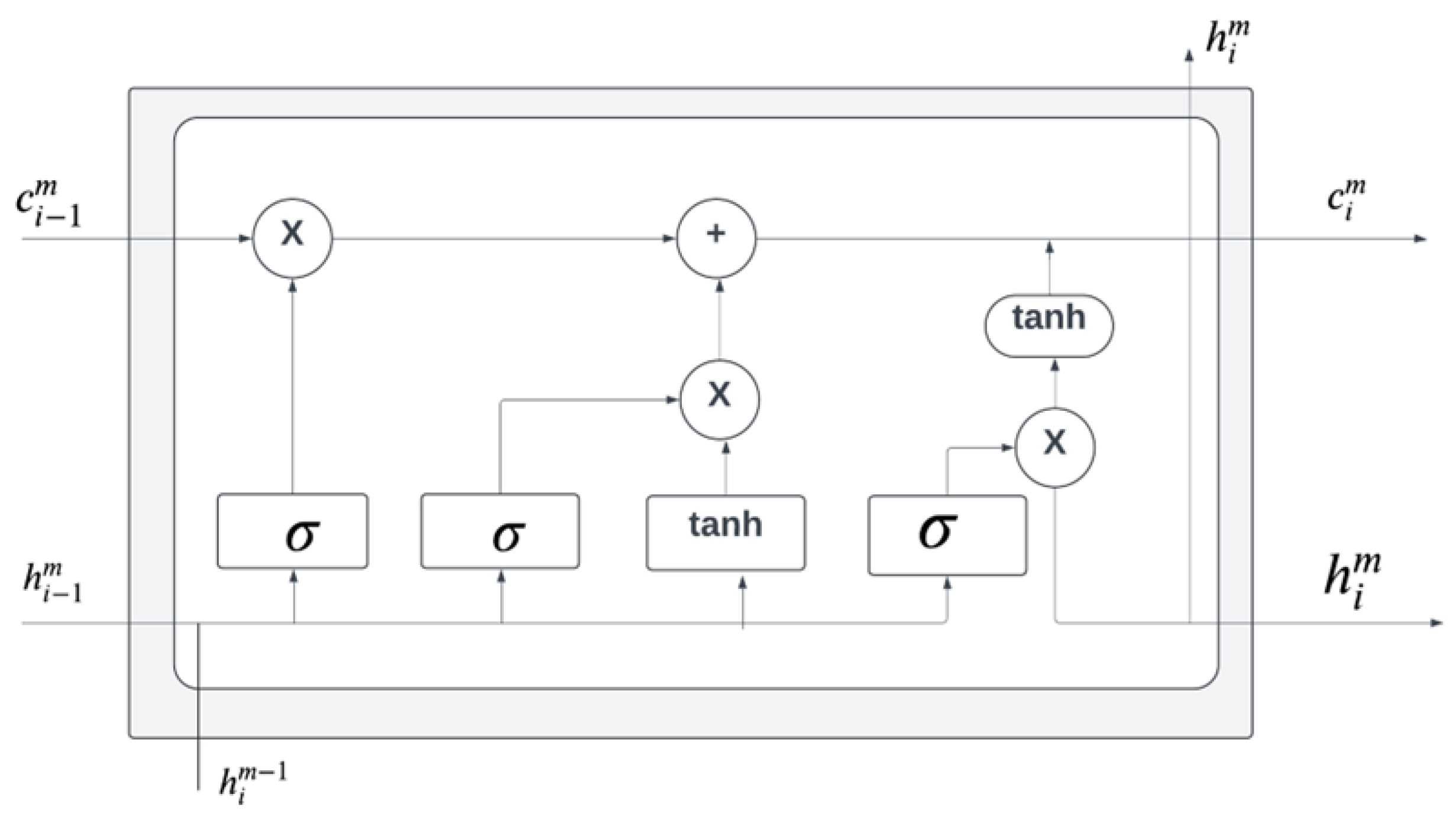
  • LSTM: A type of recurrent neural network capable of learning long-term dependencies [14].
  • CNN: A deep learning architecture particularly effective for processing grid-like data, including time series data, which can be represented as 1D grid [15].
  • Bi-LSTM: An LSTM variant that processes sequences in forward and backward directions [16].
  • CNN-Bi-M-LSTM: A hybrid model combining CNNs with bidirectional multivariate LSTMs [16].
  • CNN-M-LSTM: A hybrid model akin to our proposed architecture but without hyperparameter fine-tuning [15].
  • M-LSTM: An LSTM variant designed to handle multiple input variables simultaneously [15].
In comparison to other architectures, the CNN-M-LSTM model demonstrates a strong capacity to efficiently handle large-scale datasets and deliver reliable medium- to long-term forecasts. The M-LSTM component is computationally lighter than more complex variants, such as Bi-LSTM, while still maintaining robust temporal modeling capabilities. The integration of convolutional layers enhances the model’s ability to extract local features, capture short-term dependencies, and reduce input dimensionality through hierarchical feature abstraction. This makes them particularly effective for identifying patterns such as periodic fluctuations or local anomalies within time series data.Furthermore, electricity consumption in commercial buildings is influenced by several factors, such as weather conditions [17], occupancy rates [18], and building characteristics [19]. Among these, temperature stands out as a key parameter driving HVAC energy usage [20]. For example, the annual power use of HVAC systems can increase by up to 12.7% in hot climates due to rising temperatures, while cold climates may see a reduction of 7.4% [21]. Hence, our proposed study incorporates outdoor temperature as a key input variable to enhance the precision of electricity consumption forecasts for HVAC systems.

2. Research Gap

Recent literature highlights several persistent limitations in existing approaches to forecasting electricity consumption for HVAC systems in commercial buildings. A key issue is the widespread reliance on conventional model architectures, predominantly traditional machine learning algorithms or standalone deep learning models for both short-term and long-term forecasting tasks. While these models can perform well under controlled or narrowly defined conditions, they often lack the generalisability required to accommodate the diverse characteristics of commercial buildings, varied climatic zones, and fluctuating patterns of energy usage. This limited adaptability restricts their practical applicability in real-world environments where variability is the norm. Although hybrid deep learning architectures, such as those combining CNNs with long LSTM have shown promise in some research settings, their adoption in practice remains relatively limited. Many of these models are developed with a focus on either short-term or long-term forecasting, seldom addressing both. This compartmentalised design presents challenges for building operators and facility managers, who typically require integrated forecasting tools capable of supporting a broad spectrum of operational decisions, from real-time system adjustments to long-term energy planning. Another critical gap in the literature is the limited incorporation of thermal comfort considerations within energy forecasting frameworks. Most existing studies rely on the Predicted Mean Vote (PMV) model [22], which, despite its widespread use, requires extensive input data and assumes uniform comfort preferences among occupants. In reality, thermal comfort is highly individual and context-dependent, particularly in dynamic commercial settings. Although emerging machine learning approaches offer the potential for more personalised and scalable assessments of thermal comfort, they are rarely integrated into forecasting models. To address these challenges, this study proposes a BO CNN-LSTM hybrid model specifically designed for commercial HVAC applications. The proposed model is capable of learning and adapting to the unique energy consumption patterns of individual buildings, delivering accurate forecasts across both short and long temporal horizons, while simultaneously integrating personalised thermal comfort metrics. This approach aims to improve forecasting accuracy and enable more human-centric, adaptive, and energy-efficient HVAC control strategies. Ultimately, this work contributes toward the development of intelligent building management systems that effectively balance operational efficiency with occupant well-being.
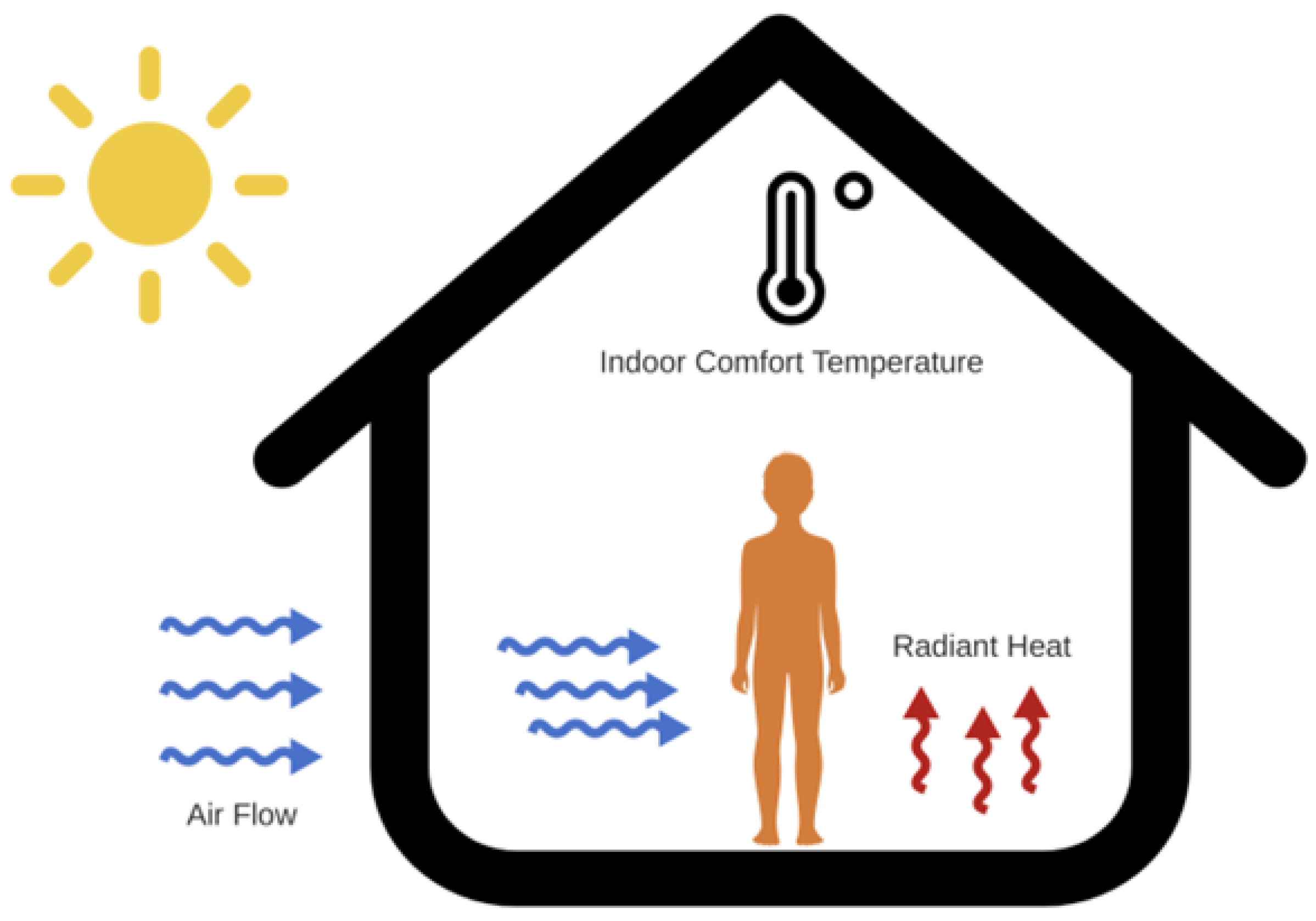
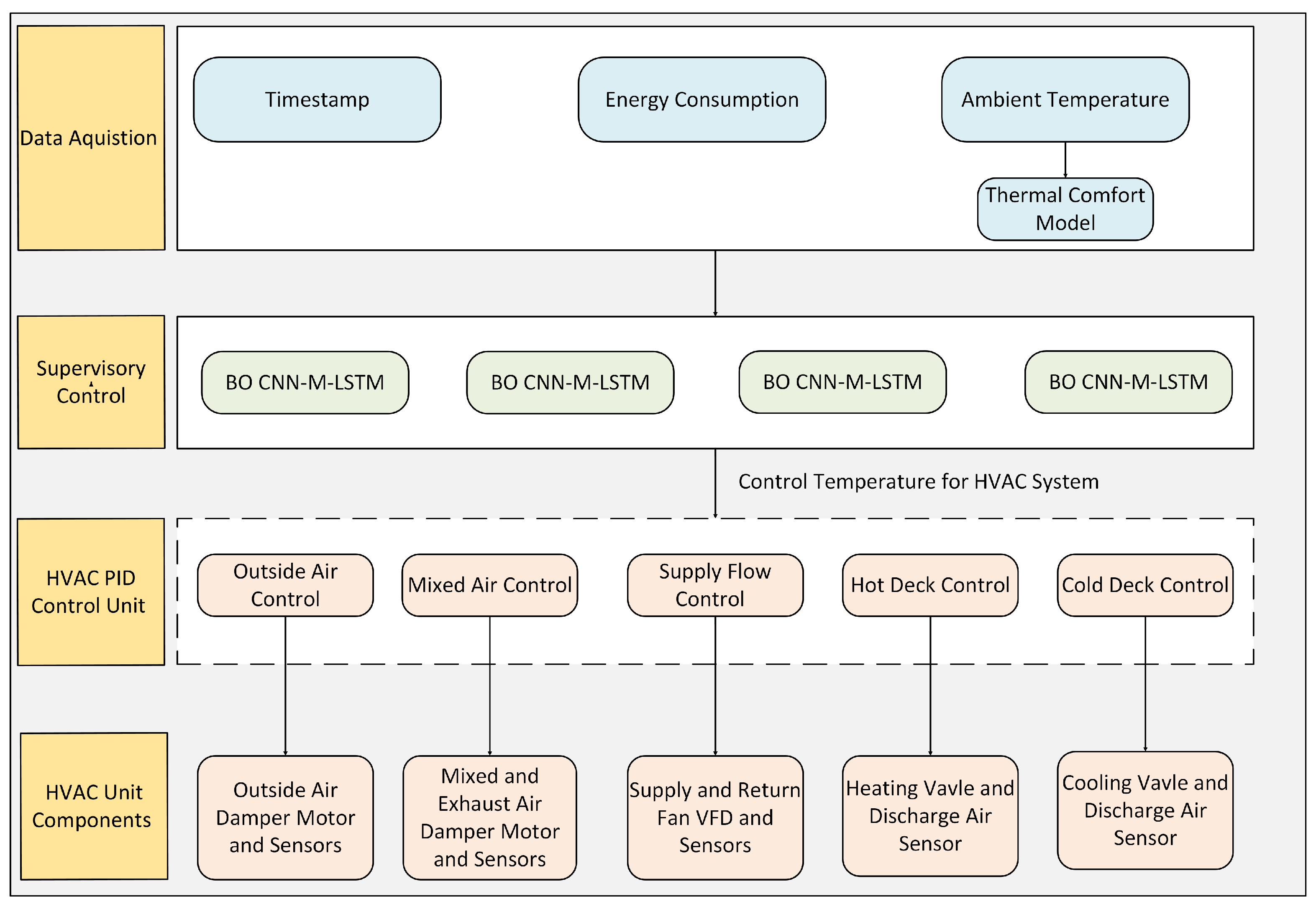
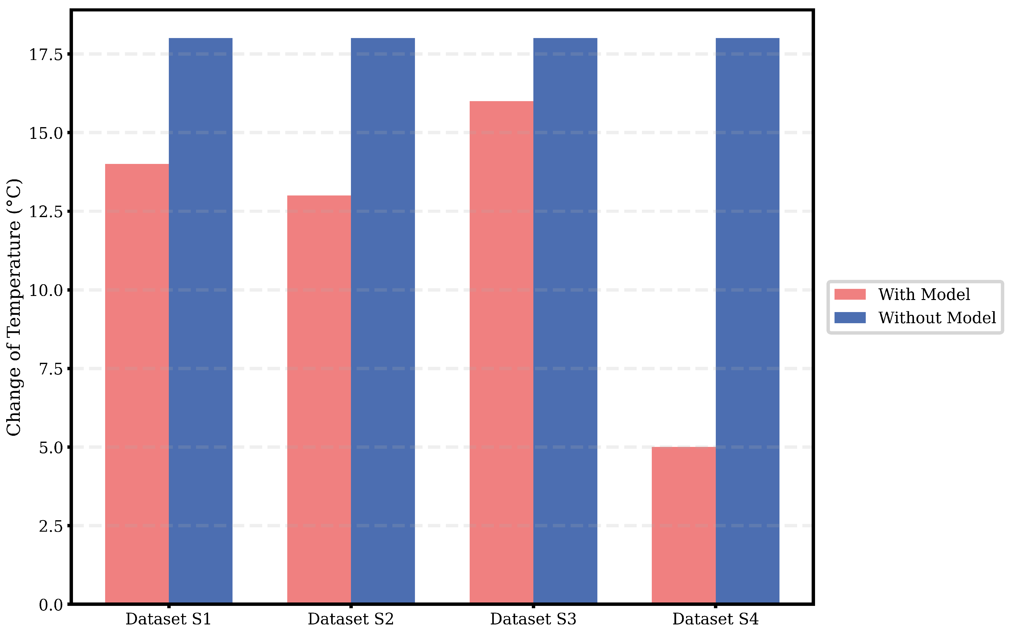
  • The proposed model optimizes indoor temperatures to enhance occupant well-being while reducing energy use and protecting building loads during peak hours. It uses an adaptive thermal comfort framework that adjusts the indoor environment in real-time based on ambient temperature. This data, combined with energy consumption and timestamps, feeds into a CNN-M-LSTM architecture for smarter climate control.
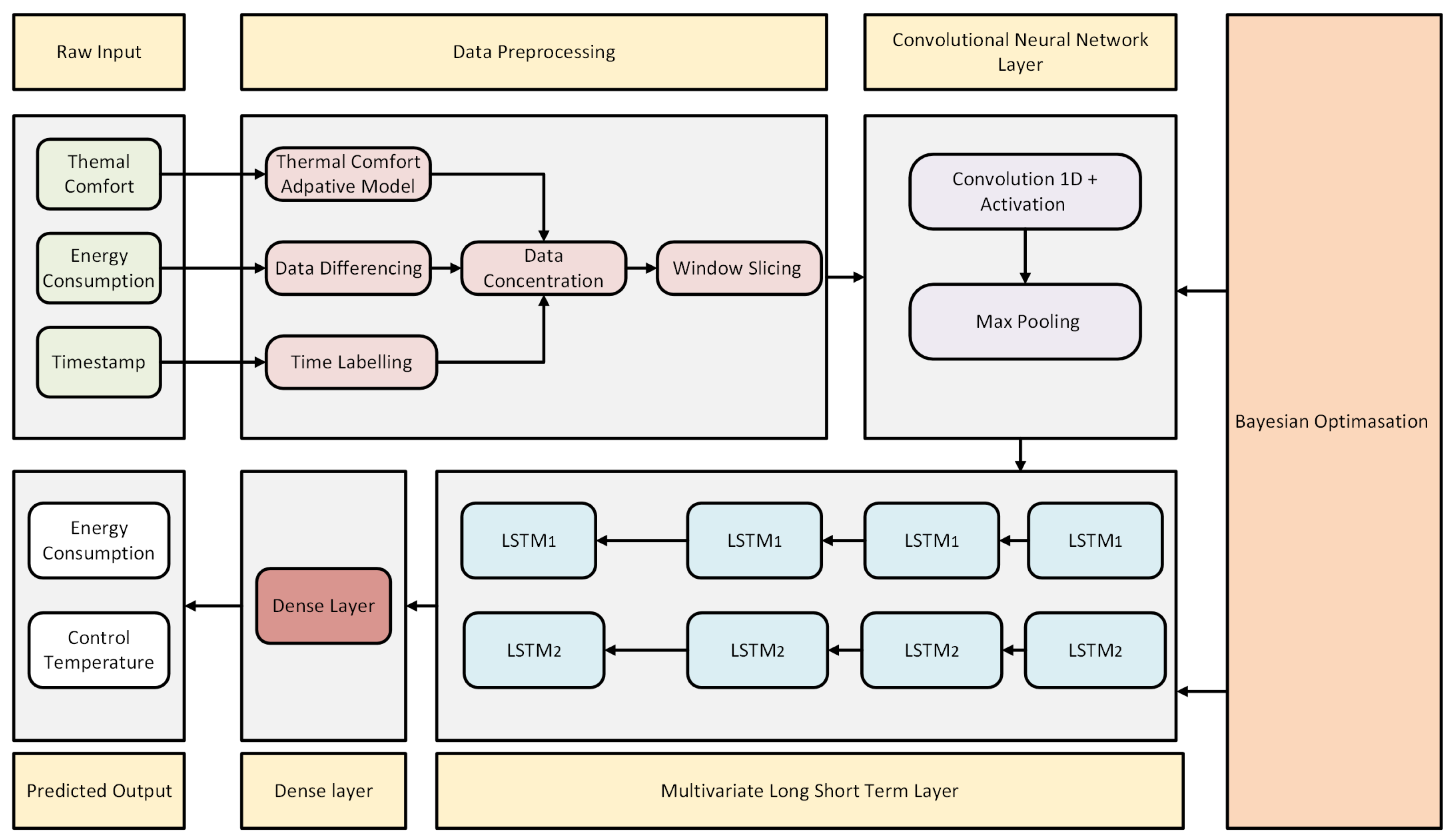
  • The CNN module is tailored to efficiently reduce dimensionality and extract critical spatial features from the input data, isolating patterns related to temperature, energy consumption, and temporal markers. Meanwhile, the M-LSTM network is specifically designed to model long-term temporal dependencies and capture trends across historical sequences. Together, this integrated architecture enables precise forecasting of future HVAC loads and indoor temperatures, leveraging the synergistic extraction of spatial and temporal features for enhanced predictive performance.
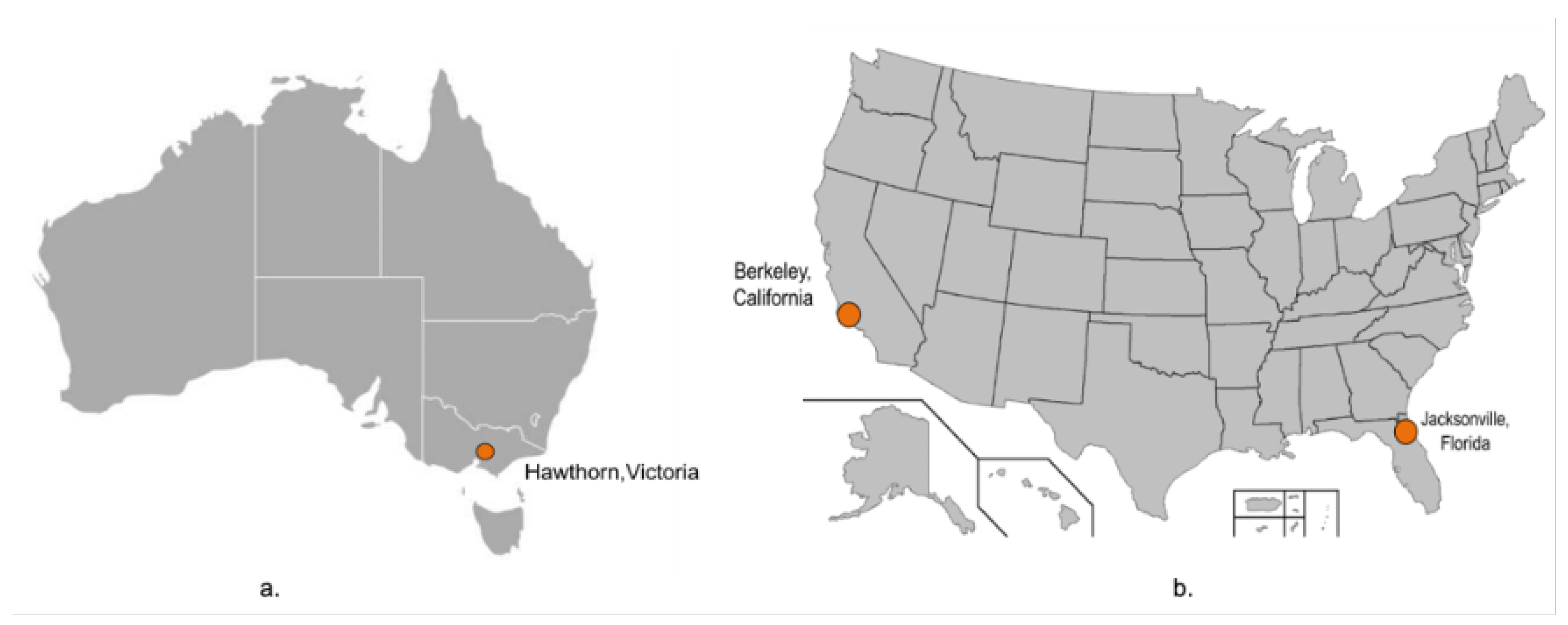
  • The proposed model uses Bayesian theory to fine-tune hyperparameters based on data characteristics. We tested it on commercial buildings in Jacksonville, Florida; Berkeley, California; and Hawthorn, Victoria. Since hotter regions (Florida, California) have higher energy use, we evaluated how well the model improves efficiency. Hawthorn’s unpredictable climate helped test its adaptability to rapid weather shifts and seasonal changes. These real-world conditions ensure the model works across different climates and building types.
This research is organized as follows: a Section 3 also introduces the thermal comfort adaptive model. Section 4 displays the data collection and processing steps, along with the architecture of the proposed and benchmark models. The Section 5 presents and discusses the experimental findings. Lastly, Section 6 summarizes the experimental results and outlines potential improvements for the proposed system.

3. Thermal Comfort Adaptive Model

Conventional heat balance models, such as the PMV and Predicted Percentage of Dissatisfied (PPD), have been widely employed to optimize HVAC operations by estimating thermal comfort levels within built environments [23]. Despite their widespread use, these models are inherently limited by their reliance on static assumptions and population averages, which often fail to reflect the temporal variability of human behavior and the influence of fluctuating ambient conditions. Moreover, the computational complexity associated with PMV-based calculations presents challenges for real-time implementation in adaptive HVAC systems. In response to these limitations, recent research has shifted towards lightweight adaptive models that dynamically incorporate occupants’ behavioral patterns and environmental feedback. These models offer a more scalable and computationally efficient solution for real-time thermal comfort control. Accordingly, linear regression and other data-driven techniques have been increasingly adopted to develop adaptive thermal comfort frameworks, as illustrated in Figure 2.
The two famous methods in thermal comfort adaptive model are Humphrey adaptive model and de Dear and Brager. The adaptive models of de Dear and Brager demonstrate better fitting with the modern architecture, which is naturally ventilated, than those of Humphrey [24]. Liu Yang et al. indicated that the R 2 of Humphrey’s model is 0.44 and that of de Dear and Brager’s model is 0.49 for naturally ventilated buildings [25,26]. Consequently, de Dear and Brager’s adaptive models have become an international standard recorded by ANSI/ASHRAE 55 [27] adaptive thermal comfort standard. However, different regions experience variations in climate. Hence, these adaptive models were adjusted to fit with the regional climate. This research proposes two variations of the de Dear and Brager adaptive model, applied to Datasets S1, S2, S3, and S4, based on the review of Q. Zhao et al. [22].
The adaptive model for Datasets S1 and S2 is expressed as follows:
T in = 17.6 + 0.31 · T out
The adaptive model for Datasets S3 and S4 is expressed as follows:
T in = 17.8 + 0.31 · T out
This study introduces two refined variations of the adaptive model, formulated for datasets S1–S4. These models define precise linear relationships between indoor thermal comfort temperature ( T in ) and ambient temperature ( T out ), ensuring enhanced applicability across diverse climatic conditions. The coefficients in the adaptive thermal comfort model were derived from regression analysis of large-scale field data. The slope 0.31 reflects how indoor comfort temperatures rise with increasing outdoor temperatures, while the intercept 17.8 and 17.6 represents the exponentially weighted running mean outdoor temperature for the day. The 17.8 °C intercept was derived from a large survey conducted in Australian environments, while 17.6 °C is based on U.S. data, as referenced in ASHRAE guidelines.

4. Methodology

This study proposes the BO CNN-M-LSTM model to optimize HVAC control in naturally ventilated commercial buildings, displayed at Figure 3. While these buildings are energy-efficient, their reliance on outdoor conditions makes temperature regulation challenging. The model forecasts energy consumption every 15 min, accounting for ambient temperature variations. By integrating BO, the CNN-M-LSTM model dynamically adjusts parameters to suit different locations, enhancing predictive accuracy. This enables better financial planning by providing energy consumption forecasts and helps commercial customers secure favorable electricity rates. Additionally, the model compares predicted and indoor temperatures, assisting HVAC systems in maintaining thermal comfort while preventing energy overloads, particularly during peak periods.

4.1. Data Collection and Preprocessing

This study utilizes datasets from four locations, each providing energy consumption and ambient temperature data over specific periods, displayed in Figure 4 and Figure 5. Dataset S1 (ATC Building, Swinburne University, Australia) and Dataset S2 (AMDC Building, Swinburne University) contain 15-min interval data from 2017 to 2019.Dataset S3 (Building 59, Lawrence Berkeley National Laboratory, USA) spans 2018–2020, while Dataset S4 (a shopping mall in Jacksonville, FL, USA) covers 2018, both recorded at 15-min intervals, displayed in Figure 6. These datasets support a comprehensive analysis of energy patterns across different climates and building types.
Energy consumption data are collected at the system level from HVAC control panels at a 15-min sampling rate. Ambient temperature in Datasets S1 and S2 is measured using four sensors placed around the building, while Datasets S3 and S4 rely on weather station reports—S3 from the Synoptic Labs station (Lawrence Berkeley National Laboratory) and S4 from Jacksonville’s local weather station. All temperature data are recorded at 15-min intervals.
In Dataset S3, temperature recordings contain both small and large data gaps. Small gaps are filled using linear interpolation to maintain consistency. However, large gaps introduce uncertainty, making interpolation unreliable. To address this, a past-week comparison strategy is employed, leveraging historical trends to reconstruct missing temperature data with greater accuracy. Specifically, a Random Forest regression model is trained on temporal and contextual features, such as time of day; energy consumption and past temperature patterns to predict and fill missing values. This approach ensures reliable temperature continuity while accounting for both temporal variability and complex.
The data processing pipeline includes five key steps: data differencing, time labeling, thermal comfort modeling, concatenation, and window slicing. Data differencing normalizes energy consumption by computing the difference between consecutive points, while time labeling marks peak hours (8 A.M.–8 P.M.) with a value of 1 and non-peak hours with 0. The thermal comfort model applies the de Dear–Brager equation to estimate adaptive comfort temperatures based on ambient conditions. These features are then combined into a single vector through concatenation, followed by window slicing, which segments the dataset into 96-point batches for training. For model development, Datasets S1 and S2 (2017–2018) were used for training, with 2019 data for testing. Dataset S3 (2018–2019) trained the model, while 2020 data served for testing. Meanwhile, Dataset S4 (January–August 2018) was used for training, and September–December 2018 for testing.

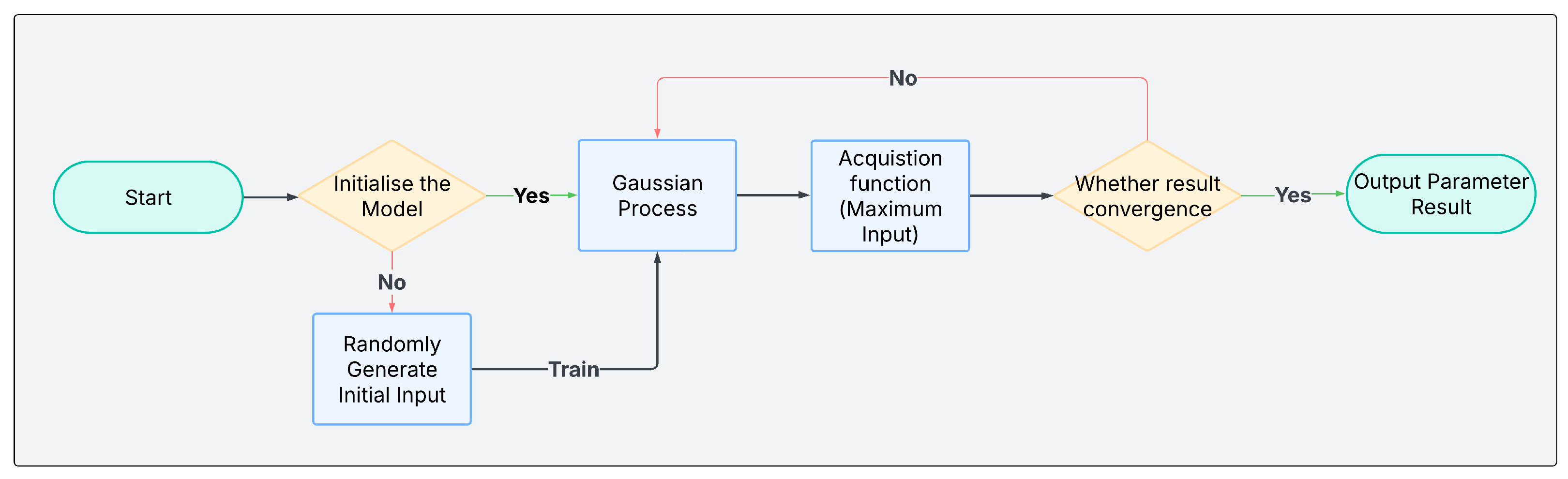
4.2. Bayesian Optimization

Bayesian optimization is applied to tune the hyperparameter and achieve the optimal performance using the specific characteristics of the datasets. Compared with grid search or Cartesian hyperparameter, Bayesian optimization can effectively perform a precision searching for optimal hyperparameter in high dimensionality [28]. It can also be used for solving non-closed form expressions. With a black box function when searching for optimal hyperparameters, Bayesian optimization combines the prior knowledge of unknown function with observed information to update a posterior information of the function distribution, as shown in Figure 7 [29]. The posterior information is updated when the optimal point is located. The core idea of Bayesian optimization can be derived as follows:
x + = arg max x A f ( x )
A Gaussian process (GP) is designed on the basis of the Gaussian stochastic process and Bayesian Learning theory to achieve the posterior information from prior knowledge [30,31]. The most important assumption of the Gaussian process is that similar inputs are likely to yield similar outputs, implying that the underlying function being modeled is smooth. A Gaussian process can be defined as follows [31]:
f ( x ) GP ( m ( x ) , k ( x , x ) )
where m(x): x R indicates the mean function, k ( x i , x j ) : x i · x j R refers to the covariance function, and f(x) denotes the unknown function. x i and x j denote the sample indices of x and y dimensions. When two sample points have strong correlation, the value of the covariance function approaches 1, and zero for weak correlation.
In the Gaussian process, the function f(x) is modeled as a collection of random variables, each following a normal distribution over all real values of f(x) [32]. The mean function is often assumed to be m(x) = 0 for simplicity, whereas the squared exponential function can be applied for the covariance function, as follows [31]:
k ( x i , x j ) = exp 1 2 x i x j 2
The acquisition function is used after the Gaussian process to search for the maximum function f(x) [31,32]. A higher acquisition function value indicates a larger value of the function f(x). The maximization of the acquisition function can be described as follows [32]:
x + = arg max x A u ( x D ) ,
where u ( x D ) indicates the acquisition function and depends on the current data D.
Several types of acquisition function are available, but this research focuses on the expected improvement (EI) function [32]. The EI function balances exploration and exploitation. For exploration, the EI function encourages investigation of uncertainty regions, facilitating the discovery of better solutions in areas with limited prior knowledge. This property is extremely important for the BO CNN-M-LSTM model due to its high-dimensional spaces [32]. For exploitation, the EI function leverages existing knowledge to refine the solutions within known regions. This strategy ensures an efficient process and reduces computation time.
The EI function EI(x) applies the maximization concept to the difference between the sampling point value f ( x + ) and the current optimum value f(x) [32]. However, if the sampling point value is smaller than the current optimum value, then the EI is defined as zero. Equation (7) derives the mathematical properties of the EI function, as follows [32]:
EI ( x ) = E [ max ( 0 , f ( x + ) f ( x ) ) ]
Bayesian optimization is a powerful technique for hyperparameter tuning, excelling in high-dimensional spaces and optimizing complex, non-closed-form functions where traditional methods like grid search often fail. Its black-box optimization capability uses prior knowledge and observed data to iteratively update posterior distributions, enabling efficient and precise tuning. This is especially important for the BO CNN-M-LSTM model, where it reduces computational costs in highly nonlinear and multidimensional settings. To support this, the hyperparameter search space is designed to enhance computational efficiency and scalability without sacrificing performance. CNN filters and LSTM units are selected in powers of two (32, 64, 128), matching hardware efficiencies and enabling scalable complexity. Kernel sizes of 3, 5, and 7 capture features at multiple spatial scales, while batch sizes of 16, 32, and 64 optimize GPU use and memory balance, facilitating faster convergence and scalable training.

4.3. Model Architecture

As shown in Figure 8, the proposed model consists of three inputs: timestamp, energy consumption, and ambient temperature. After the preprocessing stage, the CNN will extract the spatial relationships between energy consumption and ambient temperature of the HVAC system. In addition, the CNN reduces the dimensionality of the input data using pooling layers, which prevents overfitting. The CNN model block includes a 1D causal convolution layer and a max pooling layer.
In the causal convolution layer, the number of filter units is set in the range of 32 to 64 for BO. This range has been selected because the input data consists of 96 points per sequence, allowing the CNN model block to effectively extract features without risking overfitting while maintaining computational efficiency [33]. In addition, the CNN uses a kernel that creates three sliding windows to extract and capture local patterns in the data. Zero padding is added to the left side of the input to maintain the sequence structure [33].
The activation functions selected for the CNN model block include rectifier linear unit (ReLu), exponential liner unit (ELU), and leaky rectifier linear unit (Leaky ReLu). These functions introduce nonlinearity, enabling the model to capture complex patterns [34]. ReLu and Leaky ReLu are designed to mitigate the vanishing gradient problem [34]. Compared with ReLu, Leaky Relu allows for a small gradient for negative inputs [35,36]. On the contrary, ELU permits negative values for inputs, reducing bias shift and potentially accelerating convergence during training.
The characteristic equation of the casual convolution layer is described as follows [37]:
y ( n ) = i = 0 k x ( n i ) h ( i ) if n = k 1 i = 0 k x [ n i + ( s 1 ) ] h ( i ) otherwise
where x(ni) indicates the convolution length n, h(i) denotes kernel with length k, and s represents the shifted position of the kernel for every convolution performed.
The max pooling layer effectively reduces the spatial dimensions of the input feature maps while retaining the most significant information [38]. This condition is achieved by selecting the maximum value within a specified window and discarding other values. The mathematical formula is as follows [38]:
MaxPooling ( X ) i , j , k = max m , n X i · s x + m , j · s y + n , k
where X describes the input tensor; i, j, and k represent the index positions of the output tensor. m and n are used to iterate over the pooling window. s y and s x refer to the strides of the horizontal and vertical dimensions, respectively.
The M-LSTM block consists of two stacked LSTM layers, each independently capturing different levels of dependencies within the data. This structure allows the model to retain information over long periods, enhancing its ability to handle complex, nonlinear patterns between ambient temperature and energy consumption in the HVAC system [39]. The LSTM cell unit is selected by a reduction derived from the CNN model block. In particular, the unit size is halved to optimize the CPU computation and decrease the model runtime.
LSTM cells are a type of recurrent neural network (RNN) architecture, consisting of three logistic gates and one tanh function, illustrated in Figure 9. The logistic sigmoid gates and point-wise multiplication control the flow of information through the LSTM cell. Similarly, gate control decides whether information is suitable for further analysis or discarded [40]. This selective gating allows LSTM cells to manage long-term dependencies effectively and maintain stability [41]. Equation 10 derives the general mathematical formula for the output of an LSTM cell [41]:
( a j k , b j k ) = L a j 1 k , b j 1 k , a j k 1
where L receives three inputs and produces two outputs. b i m represents the output cell state, and a i m denotes the output hidden state. The three inputs are as follows: a j 1 k , the previous cell state; b j 1 k , also the previous cell state; a j k 1 , the input data.
The cell state ( b i m ) and hidden state ( a i m ) can be described as follows [42]:
b i m = f g j k · b i 1 m · u g i
a i m = o g j k · tanh ( b i m )
where the hyperbolic tangent ( t a n h ) activation function ensures that a vector of a new candidate value for the cell state remains in the range of 1 and 1.
The logistic gate comprises forget gate ( f g j k ) , input gate ( i g j k ) , and output gate ( o g j k ) . The forget gate determines which part of the cell state should be removed [41]. The input gate applies the s i g m o i d activation σ to decide which new information should be updated to the cell state. The output gate controls the value of the hidden state using information from the input and output of the previous cell [41]. Equations (13)–(15) are used to derive the mathematical behavior of the forget gate, input gate, and output gate, respectively [42].
f g j k ( a i 1 m , a i m 1 ) = σ w f g , m 1 a i m 1 w f g , m a i 1 m + b f g
i g j k ( a i 1 m , a i m 1 ) = σ w i g , m 1 a i m 1 w i g , m a i 1 m + b i g
o g j k ( a i 1 m , a i m 1 ) = σ w o g , m 1 a i m 1 w o g , m a i 1 m + b o g
where w f g , m 1  ,  w f g , m  ,  w i g , m 1 , w i g , m , w o g , m 1 , w o g , m , b f g , b i g , and b o g are the weights continuously updated during training.
The BO CNN-M-LSTM model uses the Adam optimizer for loss optimization. The Adam optimizer involves two moving averages: the gradient and the square gradient. The combination of these moving averages adjusts the learning rate dynamically for each parameter during training.

4.4. Benchmark Model

In this study, five benchmark models: BO ANN, BO CNN, BO LSTM, BO M-LSTM, BO Bi-LSTM, and BO CNN-Bi-M-LSTM are employed to evaluate the proposed BO CNN-M-LSTM model. Machine learning models were selected due to their superior capability over traditional methods in managing complex, high-dimensional datasets. Moreover, to ensure a fair and rigorous comparison, all models undergo BO for hyperparameter tuning. This consistent optimization strategy is essential, as variations in data characteristics can significantly impact model performance. By standardizing the hyperparameter tuning process, the study eliminate biases related to manual or inconsistent tuning, thereby enabling an equitable assessment of each model’s true architectural effectiveness.

4.4.1. BO ANN

The BO ANN combines hyperparameter tuning with the ANN model. The ANN model is inspired by the human neural network, consisting of hundreds of single units and weights [43]. The units in ANN cell layer 1 range from 16 to 32, and in layer 2 from 8 to 16. According to A. Vaisnav [44], Tanh and Sigmoid activations are optimal for enhancing the accuracy of hidden layers in the model. However, C. Bircanoğlu and N. Arıca illustrated that the ReLu activation is a more generic activation for ANN model hidden layers [45]. Thus, by creating a list of choices for hyperparameter tuning, Bayesian optimization is used to select the best activation based on the specific data characteristics. For the output layer, Softmax activation is applied because it is ideal for multi-class classification.

4.4.2. BO CNN

The BO CNN model is derived from the CNN block of the BO CNN-M-LSTM model, with an additional block integrated into the existing structure. The filter units in Causal Convolution Layer 1 range from 32 to 64, and in Layer 2 from 16 to 32. Furthermore, the activations for both layers include ReLu, ELU, and Leaky ReLu.

4.4.3. BO LSTM

The BO LSTM model adopts the LSTM structure from the BO CNN-M-LSTM model. The LSTM units in Layer 1 range from 8 to 64. This range ensures that the LSTM can optimize the number of units based on accuracy, as the model contains only one layer. The gradual increase in LSTM units provides better control over model capacity, and enhancing performance while preventing overfitting.

4.4.4. BO M-LSTM

The BO M-LSTM model is based on the structure of the BO CNN-M-LSTM model, with the addition of bidirectional integration applied to two LSTM layers. This improvement allows the model to capture dependencies in forward and backward directions, enhancing its ability to learn temporal patterns more effectively. The filter units in Causal Convolution Layer 1 range from 32 to 64, Layer 2 from 16 to 32 and Layer 3 range from 8 to 16. Furthermore, the activations for Casual Layer 1 include ReLu, ELU, and Leaky ReLu.

4.4.5. BO Bi-LSTM

The BO Bi-LSTM model is derived from the optimized structure of the BO CNN-M-LSTM framework, with a key enhancement being the integration of bidirectional processing across two LSTM layers. This bidirectional architecture enables the model to capture temporal dependencies in both forward and backward directions, significantly improving its ability to learn complex sequential patterns [46]. In this configuration, the number of units in the first Bi-LSTM layer is varied within a range of 8 to 64. This range is strategically selected to allow the model to adaptively determine the optimal number of units based on accuracy, given the constraint of a single Bi-LSTM layer. The incremental increase in LSTM units facilitates fine-grained control over model capacity, thereby enhancing performance while mitigating the risk of overfitting [46].

4.4.6. BO CNN-Bi-M-LSTM

The BO CNN-Bi-M-LSTM model is based on the structure of the BO CNN-M-LSTM model, with the addition of bidirectional integration applied to two LSTM layers. This improvement allows the model to capture dependencies in forward and backward directions, enhancing its ability to learn temporal patterns more effectively [46] The filter units in Causal Convolution Layer 1 range from 32 to 64, Layer 2 from 16 to 32 and Layer 3 range from 8 to 16. Furthermore, the activations for Casual Layer 1 include ReLu, ELU, and Leaky ReLu.

4.5. Model and Systematic Evaluation

The assessment of this study is structured in two phases: model evaluation and system-level evaluation. In the model evaluation phase, the predictive accuracy and reliability of the proposed model are assessed using three widely accepted metrics: Normalized Root Mean Square Error (NRMSE), Mean Absolute Percentage Error (MAPE), and the Coefficient of Determination ( R 2 ). NRMSE quantifies the average deviation between predicted and actual values, normalized by the range of the actual data [47], allowing consistent comparison across datasets of varying scales. MAPE measures the average percentage error, offering a scale-independent and interpretable indicator of forecast accuracy [47]. The R 2 score reflects the proportion of variance in the dependent variable explained by the model [47], with values approaching 1 indicating strong predictive performance. Collectively, these metrics provide a comprehensive evaluation of the model’s effectiveness. The system-level evaluation focuses on the comparison of the maximum indoor-outdoor temperature difference ( Δ T ) with and without the proposed model. This comparison is used to estimate potential energy savings. Subsequently, the average HVAC energy consumption and corresponding cost are computed to evaluate system-level benefits. The energy demand is calculated using the following heat transfer-based equation:
Q HVAC = U · A · Δ T · t COP · 1000
where the validation was carried out in a room with a floor area of 250 m2, a heat transfer coefficient (U) of 0.6 W/m2·°C, and an HVAC system operating for 12 h per day with a coefficient of performance (COP) of 3.5. During the validation test without the model, the room temperature was maintained at a constant 22 °C. Furthermore, to assess cost efficiency, the study compared the energy prices with and without the proposed model.

5. Results and Discussion

Table 2 gives the detailed comparative performance of various models concerning MAPE, NRMSE, and R 2 score. The evaluation has been performed on four different datasets in order to test their performance in the prediction concerning different conditions. For each metric, the performance of the model is compared, and the highest value in each metric across the datasets is made bold. This will clearly compare strengths and weaknesses among the models to establish the most accurate and reliable forecasting model.
In Dataset S1, Table 2, Figure 10 and Figure 11 shows the superior performance of the BO CNN-M-LSTM compared with other benchmark models. The NRMSE, MAPE, and R 2 score are 0.0322, 0.1163, and 0.8676, respectively. Compared with the BO M-LSTM model, the MAPE and R 2 score of BO CNN-M-LSTM are enhanced by 10% and 1%, respectively. Furthermore, in comparison with the BO Bi-LSTM model, the NRMSE of BO CNN-M-LSTM is improved by 2%. Figure 12 highlights the strong alignment between actual and predicted energy consumption for the BO CNN-M-LSTM model.
In Dataset S2, Table 2 and Figure 13 highlight the strong performance of the proposed BO CNN-M-LSTM model, particularly in terms of MAPE and R2 score, which reflect high prediction accuracy and strong correlation with actual values. These metrics confirm that BO CNN-M-LSTM outperforms both BO ANN and BO BI-LSTM, demonstrating its effectiveness in capturing both spatial and temporal patterns of energy consumption. However, the NRMSE metric indicates a decline in performance, with BO CNN-M-LSTM exhibiting approximately 12% higher NRMSE than BO ANN. This suggests that, despite strong average performance, the model yields larger absolute errors on certain high-magnitude samples, which substantially increase the squared error. This discrepancy is likely caused by underrepresented patterns or localized fluctuations in the training data that the model struggles to generalize. Furthermore, the complex architecture of CNN-M-LSTM may tend to overfit smooth trends while underfitting abrupt variations, leading to increased error variance. Nevertheless, as shown in Figure 14, BO CNN-M-LSTM’s predictions remain closely aligned with the actual consumption trends, reinforcing its overall robustness. To improve the NRMSE and reduce prediction variance, future work should consider increasing the number of training epochs and attending to temporal segments of the dataset to better capture extreme consumption behaviors.
In Dataset S3, Figure 15 and Figure 16 shows a strong alignment between the BO CNN-M-LSTM model and actual energy consumption. Similarly, Table 2 presents that the BO CNN-M-LSTM model outperforms all baseline models in energy consumption prediction. Compared with BO M-LSTM, the MAPE value of BO CNN-M-LSTM is reduced by 2%. For NRMSE, BO CNN-M-LSTM achieves a value of 0.0166, whereas BO Bi-LSTM stands at 0.0170, illustrating that the energy consumption prediction of BO CNN-M-LSTM is 4% closer to the actual energy consumption than BO Bi-LSTM. The R 2 score of BO CNN-M-LSTM highlights a strong correlation relationship between predicted and actual energy consumption, with an improvement of over 1% compared with BO CNN-Bi-M-LSTM.
In Dataset S4, Figure 17 and Figure 18 illustrates that the BO CNN-M-LSTM model aligns well with the actual energy consumption pattern. However, all models depict a slight decline in predictive accuracy from 30 October 2018, 12:00 P.M. to 30 November 2018, 12:00 P.M. During this time, only the BO CNN-M-LSTM and BO CNN-Bi-M-LSTM models were able to partially predict the pattern of actual energy consumption. Compared with BO CNN-Bi-LSTM, the R 2 score of BO CNN-M-LSTM is higher than 1%, depicting a strong correlation between BO CNN-M-LSTM’s predicted and actual energy consumption. As shown in Table 2, the NRMSE for BO CNN-M-LSTM is 0.0370 and 0.0380 for BO Bi-LSTM. This finding emphasizes the strong performance of BO CNN-M-LSTM over BO CNN-Bi-M-LSTM. In addition, the MAPE value of BO CNN-M-LSTM is reduced by 17% compared with BO M-LSTM. These results clearly show that the BO CNN-M-LSTM model can produce precise predictions, rendering it a highly effective approach for load forecasting.
Figure 19 illustrates the performance of the proposed model across Datasets S1 to S4. For Dataset S1, the temperature achieved with the model is 4 °C lower than without the model. Similarly, for Datasets S2, S3, and S4, the temperature reductions are 5 °C, 2 °C, and 12.5 °C, respectively. These results indicate that the model enables the HVAC system to operate in closer alignment with outdoor conditions, thereby maintaining thermal comfort and promoting occupant health by reducing temperature fluctuations. Moreover, minimizing temperature variation contributes to reduced energy consumption and improved cost efficiency, as further depicted in Table 3. With a 50% cost reduction and reduced sensitivity of indoor temperature to outdoor fluctuations, the BO CNN-M-LSTM model demonstrates a significant contribution to lowering energy consumption and enhancing occupant wellbeing in commercial buildings.

6. Conclusions

This research has introduced a method to control HVAC systems more efficiently by reducing energy consumption and satisfying occupants’ well-being. The main objective of this study is to use the BO CNN-M-LSTM to learn the relationship of energy consumption and ambient temperature recorded every 15 min, and then output the control temperature and predictive energy consumption. The CNN model block is responsible for capturing spatial information, whereas the M-LSTM model learns complex temporal patterns. The addition of hyperparameter tuning helps to adjust the parameters to best fit with the data characteristics, thereby achieving precise predictions. To improve user satisfaction, the proposed model has also integrated an adaptive thermal comfort model during the preprocessing stage to generate a sequence of comfortable indoor temperatures. Moreover, our research focused on multiple locations with different climate conditions: Datasets S1 and S2 are from Hawthorn, Victoria; Dataset S3 is from Berkeley, California; Dataset S4 is from Jacksonville, Florida. This diversity allows the model to be thoroughly tested, demonstrating its robust capabilities. The results demonstrate that the BO CNN-M-LSTM outperforms all benchmark models including BO ANN, BO CNN, BO CNN-Bi-M-LSTM, BO M-LSTM, BO LSTM, and BO Bi-LSTM. The findings show that:
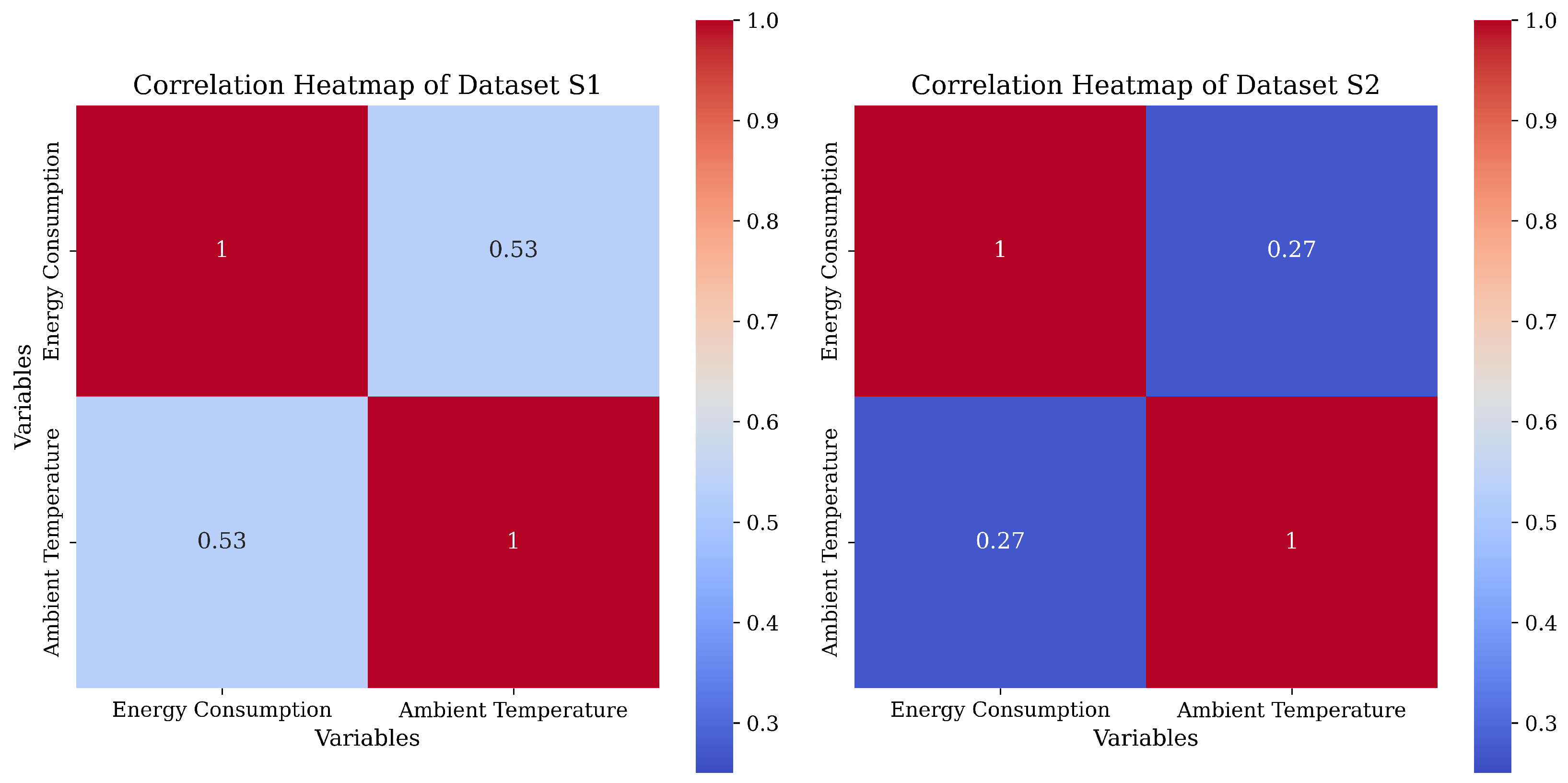
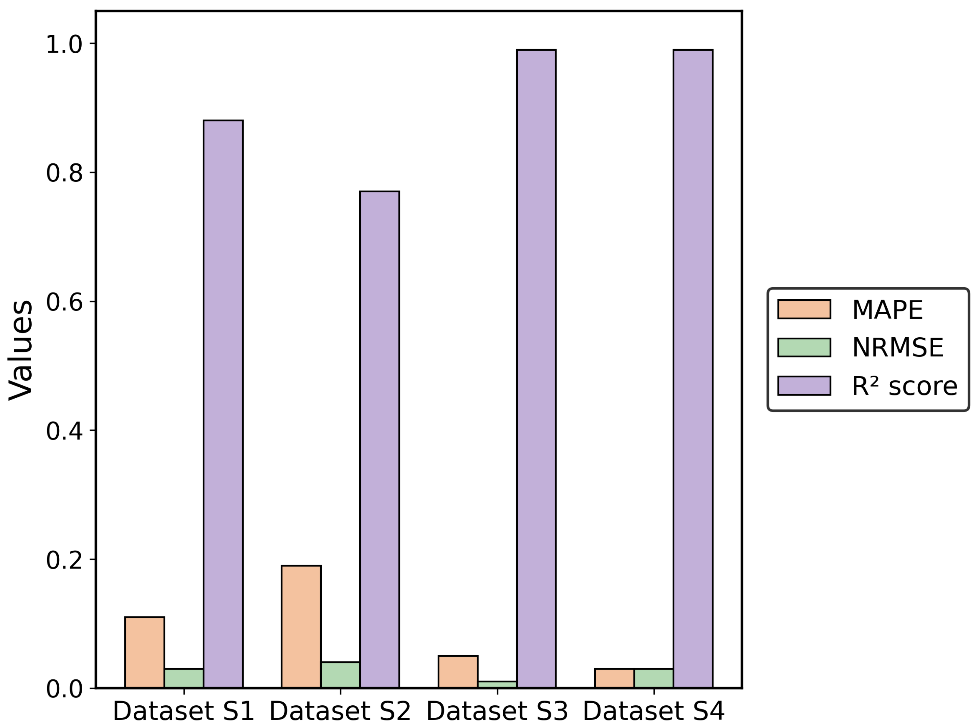
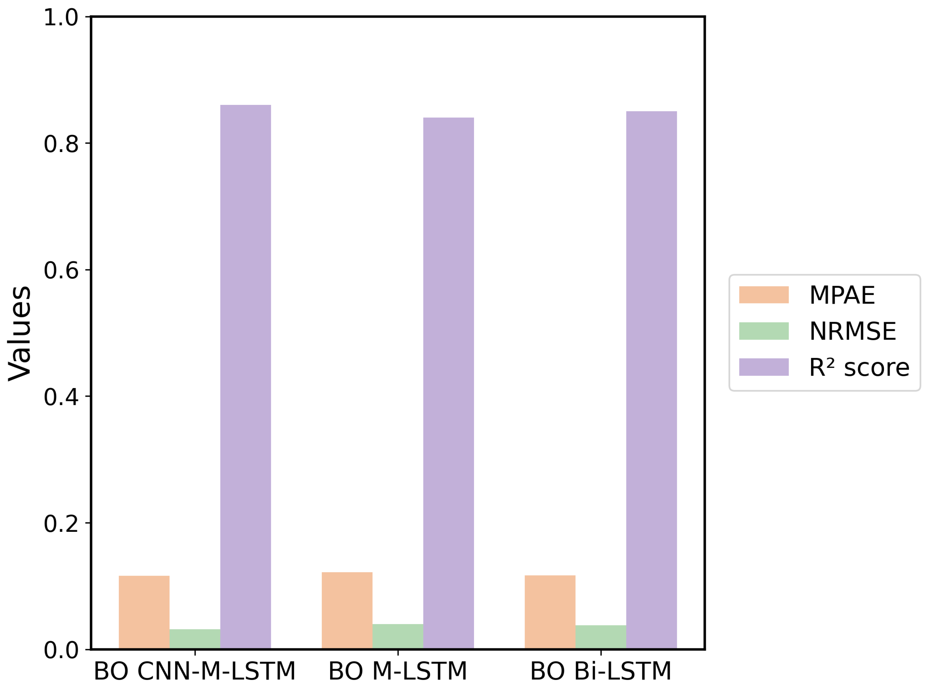
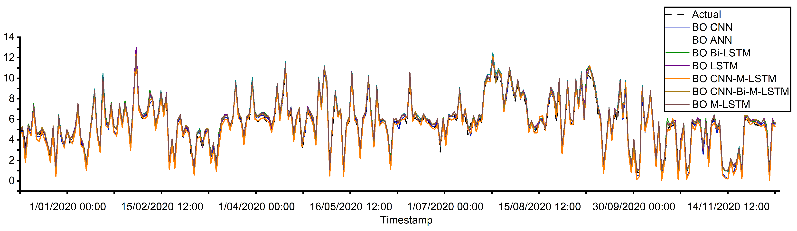
  • In Dataset S1, the MAPE value of BO CNN-M-LSTM is 0.1163, which higher than that of BO ANN by 10%. The NRMSE of BO CNN-M-LSTM and BO Bi-LSTM is 0.0322 and 0.0388, respectively. The R 2 score of BO CNN-M-LSTM is the highest at 0.8676, indicating a strong correlation between the predicted and actual energy consumption.
  • In Dataset S2, the NRMSE value of BO CNN-M-LSTM is 0.0385, which is lower than that of BO ANN by 12%. This metric indicated that the proposed model exhibits a slight increase in error variance. The MAPE of BO CNN-M-LSTM and BO CNN-Bi-M-LSTM is 0.1939 and 0.1946, respectively. Furthermore, the R 2 score of BO CNN-M-LSTM is the highest at 0.7805. This finding highlights that BO CNN-M-LSTM can produce precise energy consumption predictions, but might exhibit error variance. Hence, to improve the NRMSE metric of the proposed model, the future work can increase the training iterations.
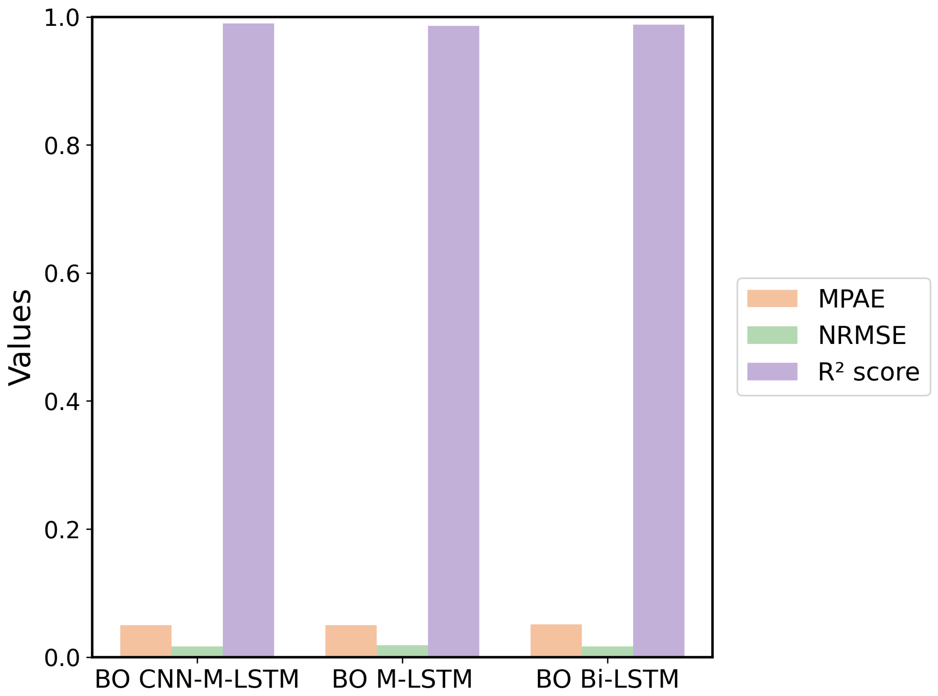
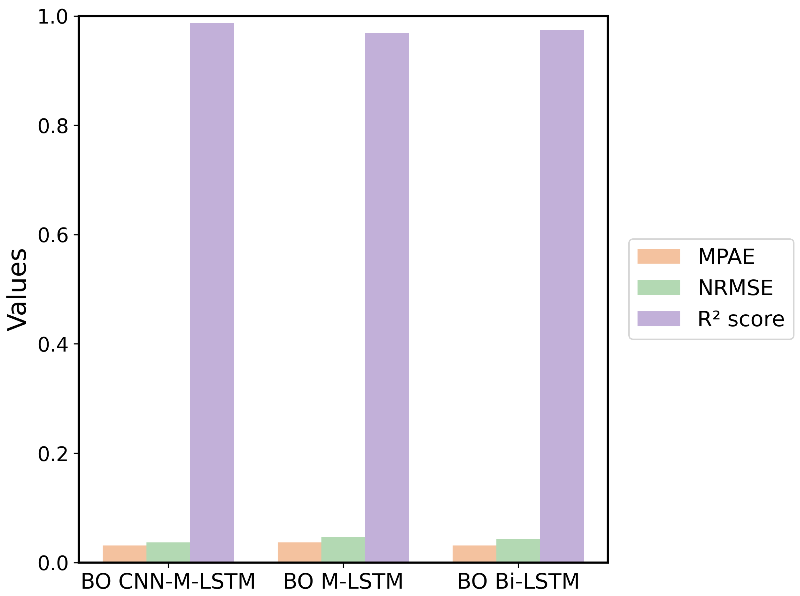
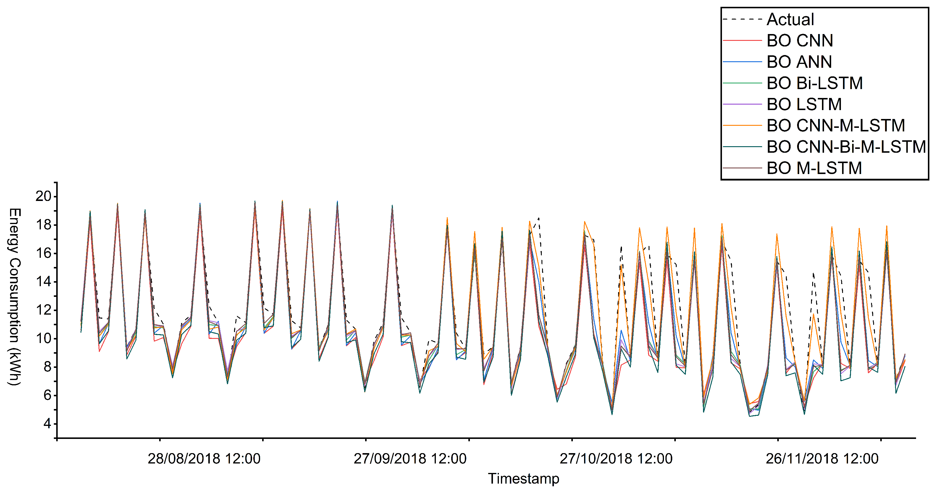
  • In Dataset S3, the MAPE value of BO CNN-M-LSTM is 0.049, which is higher than that of BO M-LSTM by 1%. The NRMSE of BO CNN-M-LSTM is 0.0166, and that of BO Bi-LSTM is 0.0170. The R 2 score of BO CNN-M-LSTM is the highest at 0.9896. This finding shows a strong correlation between the predicted and actual energy consumption.
  • In Dataset S4, the NRMSE value of BO CNN-M-LSTM is 0.0370, which is better than BO M-LSTM by 3%. The MAPE of BO CNN-M-LSTM is 0.0311, and that of BO Bi-LSTM is 0.0313. The R 2 score of BO CNN-M-LSTM is the highest at 0.9872. This result indicates a proportional relationship between the predicted and actual energy consumption.
Overall, the experiment highlights the strong performance of the BO CNN-M-LSTM model, demonstrating its capability to generate accurate predictions across varying climate conditions. Despite some performance degradation observed in Dataset S2, the model remains effective and reliable for forecasting HVAC loads in commercial buildings. Notably, the proposed approach achieves up to a 50% reduction in energy-related costs while mitigating the impact of outdoor temperature fluctuations on indoor environments, thereby enhancing occupant comfort and wellbeing. To further improve the performance and practical applicability of the proposed model, several directions can be considered for future work. One promising approach involves incorporating real-time feedback from building occupants via IoT-enabled sensors. This would allow the system to account for individual thermal preferences, thereby enabling more adaptive and user-centered control strategies. In addition, enriching the input data with supplementary environmental features, such as indoor humidity levels, occupancy trends, and air quality metrics could provide the model with a more comprehensive understanding of building conditions, ultimately enhancing prediction accuracy. Furthermore, applying transfer learning techniques may improve the model’s ability to generalise to unseen buildings or geographic regions, particularly in scenarios where data availability is limited. Finally, deploying the model on edge computing platforms and testing its performance in live, operational HVAC systems would represent a critical step toward validating its robustness, scalability, and real-world utility.

Author Contributions

Conceptualization, C.N.L. and T.N.D.; methodology, C.N.L.; software, C.N.L.; validation, C.N.L., T.N.D. and A.V.; formal analysis, C.N.L.; investigation, C.N.L.; resources, A.S. and J.C.; data curation, S.S.; writing—original draft preparation, C.N.L.; writing—review and editing, A.V.; visualization, C.N.L.; supervision, T.N.D., J.C. and A.V.; project administration, S.S.; funding acquisition, A.S. and J.C. All authors have read and agreed to the published version of the manuscript.

Funding

This research received no external funding.

Institutional Review Board Statement

Not applicable.

Informed Consent Statement

Not applicable.

Data Availability Statement

Data is available from GitHub link: https://github.com/chinghiep01/HVAC-System-Data (accessed on 27 May 2025).

Acknowledgments

Special thanks to our colleagues and collaborators for their valuable insights and constructive feedback throughout the study. We also appreciate the assistance provided by the technical and administrative staff in facilitating data collection and experimental setup. Finally, we extend our heartfelt appreciation to our families and friends for their unwavering support and encouragement during this research endeavor.

Conflicts of Interest

The authors declare no conflicts of interest.

Abbreviations

The following abbreviations are used in this manuscript:
SVMSupervised Vector Machine
ANNArtificial Neural Network
DDPGDeep Deterministic Policy Gradient
CNNConvolutional Neural Network
LSTMLong Short-Term Memory
Bi-LSTMBidirectional Long Short-Term Memory
AE-DDPGAutoencoder-Deep Deterministic Policy Gradient
ED-LSTM with MPEncoder-Decoder LSTM with Multi-Layer Perceptron
ED-LSTM with SMPEncoder-Decoder LSTM with Shared Multi-Layer Perceptron

References

  1. International Energy Agency. Buildings-Energy System; IEA: Paris, France, 11 July 2023; Available online: https://www.iea.org/energy-system/buildings (accessed on 3 February 2025).
  2. U.S. Energy Information Administration. Consumption & Efficiency—U.S. Energy Information Administration (EIA). December 2022. Available online: https://www.eia.gov/consumption/commercial/data/2018/pdf/CBECS%202018%20CE%20Release%202%20Flipbook.pdf (accessed on 3 February 2025).
  3. Tejjy Incorporation. How HVAC System Works: Basic Functionality & Types; Tejjy Inc.: Rockville, MD, USA, 2024; Available online: https://www.tejjy.com/hvac-system-work/ (accessed on 9 December 2024).
  4. Jurjevic, R.; Zakula, T. Demand Response in Buildings: A Comprehensive Overview of Current Trends, Approaches, and Strategies. Buildings 2023, 13, 2663. [Google Scholar] [CrossRef]
  5. Agouzoul, A.; Simeu, E. Predictive Control Method for Comfort and Thermal Energy Enhancement in Buildings. In Proceedings of the 2024 International Conference on Computer-Aided Design (ICCAD), Paris, France, 15–17 May 2024. [Google Scholar] [CrossRef]
  6. Wang, H.; Wang, S.; Tang, R. Development of grid-responsive buildings: Opportunities, challenges, capabilities and applications of HVAC systems in non-residential buildings in providing ancillary services by fast demand responses to smart grids. Appl. Energy 2019, 250, 697–712. [Google Scholar] [CrossRef]
  7. Goodman, D.; Chen, J.; Razban, A.; Li, J. Identification of Key Parameters Affecting Energy Consumption of an Air Handling Unit. In Proceedings of the ASME 2016 International Mechanical Engineering Congress and Exposition (IMECE2016), Phoenix, AZ, USA, 11–17 November 2016. [Google Scholar] [CrossRef]
  8. Bengea, S.C.; Kelman, A.D.; Borrelli, F.; Taylor, R.; Narayanan, S. Implementation of model predictive control for an HVAC system in a mid-size commercial building. HVAC&R Res. 2014, 20, 121–135. [Google Scholar] [CrossRef]
  9. Zheng, P.; Wu, H.; Liu, Y.; Ding, Y.; Yang, L. Thermal Comfort in Temporary Buildings: A Review. Buildings 2022, 221, 109262. [Google Scholar] [CrossRef]
  10. Wang, H.; Mai, D.; Li, Q.; Ding, Z. Evaluating Machine Learning Models for HVAC Demand Response: The Impact of Prediction Accuracy on Model Predictive Control Performance. Buildings 2024, 14, 2212. [Google Scholar] [CrossRef]
  11. Liu, T.; Xu, C.; Guo, Y.; Chen, H. A novel deep reinforcement learning based methodology for short-term HVAC system energy consumption prediction. Int. J. Refrig. 2019, 107, 39–51. [Google Scholar] [CrossRef]
  12. Mohan, D.P.; Subathra, M. A comprehensive review of various machine learning techniques used in load forecasting. Recent Adv. Electr. Electron. Eng. 2022, 16, 197–210. [Google Scholar] [CrossRef]
  13. Liu, J.; Zhai, Z.; Zhang, Y.; Wang, Y.; Ding, Y. Comparison of energy consumption pre-diction models for air conditioning at different time scales for large public buildings. J. Build. Eng. 2024, 96, 110423. [Google Scholar] [CrossRef]
  14. Lara-Benítez, P.; Carranza-García, M.; Riquelme, J.C. An Experimental Review on Deep Learning Architectures for Time Series Forecasting. Int. J. Neural Syst. 2021, 31, 2130001. [Google Scholar] [CrossRef]
  15. Agga, F.A.; Abbou, S.A.; Houm, Y.E.; Labbadi, M. Short-Term Load Forecasting Based on CNN and LSTM Deep Neural Networks. IFAC-PapersOnLine 2022, 55, 777–781. [Google Scholar] [CrossRef]
  16. Bohara, B.; Fernandez, R.; Gollapudi, V.; Li, X. Short-Term Aggregated Residential Load Forecasting using BiLSTM and CNN-BiLSTM. In Proceedings of the 2022 International Conference on Innovation and Intelligence for Informatics, Computing, and Technologies (3ICT), Sakheer, Bahrain, 20–21 November 2022. [Google Scholar] [CrossRef]
  17. Li, H.; Dai, Y.; Liu, X.; Zhang, T.; Zhang, J.; Liu, X. Feature extraction and an interpretable hierarchical model for annual hourly electricity consumption profile of commercial buildings in China. Energy Convers. Manag. 2023, 291, 117244. [Google Scholar] [CrossRef]
  18. Reveshti, A.M.; Khosravirad, E.; Rouzbahani, A.K.; Fariman, S.K.; Najafi, H.; Peivan-dizadeh, A. Energy consumption prediction in an office building by examining occupancy rates and weather parameters using the moving average method and artificial neural network. Heliyon 2024, 10, e25307. [Google Scholar] [CrossRef]
  19. Afroz, Z.; Goldsworthy, M.; White, S.D. Energy flexibility of commercial buildings for demand response applications in Australia. Energy Build. 2023, 300, 113533. [Google Scholar] [CrossRef]
  20. Mayer, P.; Meyer, W.; Nussbaum, R. Performance of Demand Side Management for Building HVAC Systems. In Proceedings of the 2009 IEEE Power and Energy Society General Meeting, Calgary, AB, Canada, 26–30 July 2009; pp. 1–6. [Google Scholar]
  21. Kharseh, M.; Altorkmany, L.; Al-Khawaj, M.; Hassani, F. Warming impact on energy use of HVAC system in buildings of different thermal qualities and in different climates. Energy Convers. Manag. 2014, 81, 106–111. [Google Scholar] [CrossRef]
  22. Zhao, Q.; Lian, Z.; Lai, D. Thermal comfort models and their developments: A review. Energy Built Environ. 2021, 2, 21–33. [Google Scholar] [CrossRef]
  23. de Vet, E.; Head, L. Everyday weather-ways: Negotiating the temporalities of home and work in Melbourne, Australia. Geoforum 2020, 108, 267–274. [Google Scholar] [CrossRef]
  24. de Dear, R.; Brager, G.S. Developing an Adaptive Model of Thermal Comfort and Preference. Escholarship. 2017. Available online: https://escholarship.org/uc/item/4qq2p9c6 (accessed on 12 February 2025).
  25. Yang, L.; Yan, H.; Lam, J.C. Thermal comfort and building energy consumption implica-tions—A review. Appl. Energy 2014, 115, 164–173. [Google Scholar] [CrossRef]
  26. Yao, R.; Zhang, S.; Du, C.; Schweiker, M.; Hodder, S.; Olesen, B.W.; Toftum, J.; d’Ambrosio, F.R.; Gebhardt, H.; Zhou, S.; et al. Evolution and performance analysis of adaptive thermal comfort models—A comprehensive literature review. Build. Environ. 2022, 217, 109020. [Google Scholar] [CrossRef]
  27. ANSI/ASHRAE Standard 55-2020; Thermal Environmental Conditions for Human Occupancy. ASHRAE: Atlanta, GA, USA, 2020.
  28. Alibrahim, H.; Ludwig, S.A. Hyperparameter Optimization: Comparing Genetic Algorithm against Grid Search and Bayesian Optimization. In Proceedings of the 2021 IEEE Congress on Evolutionary Computation (CEC), Kraków, Poland, 28 June–1 July 2021; pp. 1551–1559. [Google Scholar] [CrossRef]
  29. Wu, J.; Chen, X.-Y.; Zhang, H.; Xiong, L.-D.; Lei, H.; Deng, S.-H. Hyperparameter Optimization for Machine Learning Models Based on Bayesian Optimization. J. Electron. Sci. Technol. 2019, 17, 26–40. [Google Scholar]
  30. Cho, H.; Kim, Y.; Lee, E.; Choi, D.; Lee, Y.; Rhee, W. Basic Enhancement Strategies When Using Bayesian Optimization for Hyperpa-rameter Tuning of Deep Neural Networks. IEEE Access 2020, 8, 52588–52608. [Google Scholar] [CrossRef]
  31. Klein, A.; Falkner, S.; Bartels, S.; Hennig, P.; Hutter, F. Fast Bayesian Optimization of Machine Learning Hyperparameters on Large Da-tasets. In Proceedings of the 20th International Conference on Artificial Intelligence and Statistics, Fort Lauderdale, FL, USA, 20–22 April 2017; pp. 528–536. Available online: https://proceedings.mlr.press/v54/klein17a.html (accessed on 12 February 2025).
  32. Zulfiqar, M.; Gamage, K.A.A.; Kamran, M.; Rasheed, M.B. Hyperparameter Optimization of Bayesian Neural Network Using Bayesian Optimization and Intelligent Feature Engineering for Load Forecasting. Sensors 2022, 22, 4446. [Google Scholar] [CrossRef] [PubMed]
  33. Aloysius, N.; Geetha, M. A review on deep convolutional neural networks. In Proceedings of the 2017 International Conference on Communication and Signal Processing (ICCSP), Chennai, India, 6–8 April 2017; pp. 588–592. [Google Scholar] [CrossRef]
  34. Hao, W.; Yizhou, W.; Yaqin, L.; Zhili, S. The Role of Activation Function in CNN. In Proceedings of the 2020 2nd International Con-ference on Information Technology and Computer Application (ITCA), Guangzhou, China, 18–20 December 2020; pp. 429–432. [Google Scholar] [CrossRef]
  35. Tomar, A.; Patidar, H. Analysis of Activation Function in the Convolution Neural Network Model (Best Activation Function Sigmoid or Tanh). Comput. Res. Dev. 2020, 20, 61–65. [Google Scholar]
  36. Mastromichalakis, S. ALReLU: A Different Approach on Leaky ReLU Activation Function to Improve Neural Networks Performance. arXiv 2020, arXiv:2012.07564. [Google Scholar]
  37. Alhussein, M.; Aurangzeb, K.; Haider, S.I. Hybrid CNN-LSTM Model for Short-Term Individual Household Load Forecasting. IEEE Access 2020, 8, 180544–180557. [Google Scholar] [CrossRef]
  38. Guo, X.; Zhao, Q.; Zheng, D.; Ning, Y.; Gao, Y. A Short-Term Load Forecasting Model of Multi-Scale CNN-LSTM Hybrid Neural Network Considering the Real-Time Electricity Price. Energy Rep. 2020, 6 (Suppl. 9), 1046–1053. [Google Scholar] [CrossRef]
  39. Dinh, T.N.; Thirunavukkarasu, G.S.; Seyedmahmoudian, M.; Mekhilef, S.; Stojcevski, A. Ro-bust-mv-M-LSTM-CI: Robust Energy Consumption Forecasting in Commercial Buildings during the COVID-19 Pandemic. Sustainability 2024, 16, 6699. [Google Scholar] [CrossRef]
  40. Garcia, C.I.; Grasso, F.; Luchetta, A.; Piccirilli, M.C.; Paolucci, L.; Talluri, G. A Comparison of Power Quality Disturbance Detection and Classification Methods Using CNN, LSTM and CNN-LSTM. Appl. Sci. 2020, 10, 6755. [Google Scholar] [CrossRef]
  41. Sherstinsky, A. Fundamentals of Recurrent Neural Network (RNN) and Long Short-Term Memory (LSTM) Network. Phys. D Nonlinear Phenom. 2020, 404, 132306. [Google Scholar] [CrossRef]
  42. Nichiforov, C.; Stamatescu, G.; Stamatescu, I.; Făgărăşan, I. Evaluation of Sequence-Learning Models for Large-Commercial-Building Load Forecasting. Information 2019, 10, 189. [Google Scholar] [CrossRef]
  43. Jing, Z.; Cai, M.; Pipattanasomporn, M.; Rahman, S.; Kothandaraman, R.; Malekpour, A.; Paaso, E.A.; Bahramirad, S. Commercial Building Load Forecasts with Artificial Neural Network. In Proceedings of the 2019 IEEE Power & Energy Society Innovative Smart Grid Technologies Conference (ISGT), Washington, DC, USA, 18–21 February 2019; pp. 1–5. [Google Scholar] [CrossRef]
  44. Vaisnav, A.; Ashok, S.; Vinaykumar, S.; Thilagavathy, R. FPGA Implementation and Comparison of Sigmoid and Hyperbolic Tangent Activation Functions in an Artificial Neural Network. In Proceedings of the 2022 International Conference on Electrical, Computer and Energy Technologies (ICECET), Prague, Czech Republic, 20–22 July 2022; pp. 1–4. [Google Scholar] [CrossRef]
  45. Bircanoğlu, C.; Arıca, N. A Comparison of Activation Functions in Artificial Neural Networks. In Proceedings of the 2018 26th Signal Processing and Communications Applications Conference (SIU), Izmir, Turkey, 2–5 May 2018; pp. 1–4. [Google Scholar] [CrossRef]
  46. Cai, C.; Tao, Y.; Zhu, T.; Deng, Z. Short-term load forecasting based on deep learning bidirectional LSTM neural network. Appl. Sci. 2021, 11, 8129. [Google Scholar] [CrossRef]
  47. Piotrowski, P.; Rutyna, I.; Baczyński, D.; Kopyt, M. Evaluation Metrics for Wind Power Forecasts: A Comprehensive Review and Statistical Analysis of Errors. Energies 2022, 15, 9657. [Google Scholar] [CrossRef]
Figure 1. HVAC System in Commercial Buildings.
Designs 09 00069 g001
Figure 2. Thermal Comfort in Commercial Buildings.
Designs 09 00069 g002
Figure 3. Proposed Design of a Predictive Model for HVAC Control System.
Designs 09 00069 g003
Figure 4. Correlation Heatmap of Dataset S1 and S2.
Designs 09 00069 g004
Figure 5. Correlation Heatmap of Dataset S3 and S4.
Designs 09 00069 g005
Figure 6. Location of all the datasets: (a). Dataset S1 and S2 location and (b). Dataset S3 and S4 location.
Designs 09 00069 g006
Figure 7. Bayesian Optimization Process Flow Chart.
Designs 09 00069 g007
Figure 8. BO CNN-M-LSTM architecture.
Designs 09 00069 g008
Figure 9. LSTM cell architecture.
Designs 09 00069 g009
Figure 10. The performance of BO CNN-M-LSTM evaluated across different datasets.
Designs 09 00069 g010
Figure 11. Comparison of BO CNN-M-LSTM with the top 3 models across datasets S1.
Designs 09 00069 g011
Figure 12. Prediction for energy consumption of all models for Dataset S1.
Designs 09 00069 g012
Figure 13. Comparison of BO CNN-M-LSTM with the top 3 models across datasets S2.
Designs 09 00069 g013
Figure 14. Prediction for enrgy consumption of all models for Dataset S2.
Designs 09 00069 g014
Figure 15. Comparison of BO CNN-M-LSTM with the top 3 models across datasets S3.
Designs 09 00069 g015
Figure 16. Prediction for energy consumption of all models for Dataset S3.
Designs 09 00069 g016
Figure 17. Comparison of BO CNN-M-LSTM with the top 3 models across datasets S4.
Designs 09 00069 g017
Figure 18. Prediction for energy consumption of all models for Dataset S4.
Designs 09 00069 g018
Figure 19. Maximum change of outdoor and indoor temperature with and without proposed model.
Designs 09 00069 g019
Table 1. Overview of various models for electricity consumption forecasting of HVAC systems in commercial buildings.
IDForecasting ModelYearForecasting HorizonRMSEMAE R 2 Score
1SVM [11]202410 min ahead35,189 W25,653 W0.930
2ANN [11]202410 min ahead24,704 W18,081 W0.966
3XGBoost [11]202410 min ahead16,149 W11,354 W0.978
4LightGBM [11]202410 min ahead24,218 W15,827 W0.967
5DDPG [12]20195 min ahead19.092%3.858%0.992
6AE-DDPG [12]20195 min ahead15.321%3.470%0.992
7ED-LSTM with MP  [13]201783 days ahead15.400%
8ED-LSTM with SMP  [13]201783 days ahead 11.200%
Table 2. Model Performance Metrics for Different Datasets.
DatasetModelMetricsMetric Values
MPAENRMSE R 2 Score
Dataset S1BO CNN-M-LSTM 0.11630.03220.8676
BO CNN 0.12590.03980.8551
BO ANN 0.11770.03650.8625
BO M-LSTM 0.12480.04080.8478
BO LSTM 0.13240.04290.8315
BO CNN-Bi-M-LSTM 0.12440.04040.8505
BO Bi-LSTM 0.11760.03880.8625
Dataset S2BO CNN-M-LSTM 0.19390.03850.7805
BO CNN 0.27440.04270.7297
BO ANN 0.19640.03390.7788
BO M-LSTM 0.20520.04200.7376
BO LSTM 0.22560.04190.7388
BO CNN-Bi-M-LSTM 0.19460.03940.7692
BO Bi-LSTM 0.19640.03860.7788
Dataset S3BO CNN-M-LSTM 0.04990.01660.9896
BO CNN 0.10020.04490.9221
BO ANN 0.05100.02320.9880
BO M-LSTM 0.05000.01890.9861
BO LSTM 0.05700.02450.9768
BO CNN-Bi-M-LSTM 0.05790.02240.9806
BO Bi-LSTM 0.05110.01700.9880
Dataset S4BO CNN-M-LSTM 0.03110.03700.9872
BO CNN 0.06730.05360.9590
BO ANN 0.03130.03990.9739
BO M-LSTM 0.03710.04710.9684
BO LSTM 0.03900.04940.9652
BO CNN-Bi-M-LSTM 0.03990.03800.9794
BO Bi-LSTM 0.03130.04280.9739
Table 3. Average Energy Consumption and Operating Cost per hour.
Average Energy Consumption (kWH)Average Operating Cost ($)
With Model6.241.63
Without Model11.312.93
Disclaimer/Publisher’s Note: The statements, opinions and data contained in all publications are solely those of the individual author(s) and contributor(s) and not of MDPI and/or the editor(s). MDPI and/or the editor(s) disclaim responsibility for any injury to people or property resulting from any ideas, methods, instructions or products referred to in the content.

