Dual-Level Fault-Tolerant FPGA-Based Flexible Manufacturing System

Abstract

This paper proposes a fault-tolerant flexible manufacturing system (FMS) that features a dual-level fault tolerance mechanism at both the workcell and system levels to enhance reliability. The workcell controller was implemented on a Field Programmable Gate Array (FPGA). Reconfigurable duplication was used as the first level of fault tolerance at the workcell level. It was shown how to detect and recover from FPGA faults such as Single Event Upsets (SEUs), hard faults, and Single Event Functional Interrupts (SEFIs). The prototype of the workcell controller was successfully implemented using two Zybo Z7-20 AMD boards and an Arduino DUE. Petri Nets were used to prove that controller reliability increased by 346% after 1440 operational hours. The second level of fault tolerance was at the FMS level; the Supervisor (SUP) took over the responsibilities of any malfunctioning workcell controller. Riverbed software was used to prove that the system successfully met the end-to-end delay requirements. Finally, Matlab showed that there is a further increase in performability.

1. Introduction

FMSs were introduced in the 1960s by Williamson, who is regarded as the pioneer of FMSs, which played a pivotal role in revolutionizing production through the introduction of numerically controlled (NC) machine tools and the use of computers to control manufacturing processes. However, in the 1970s, the first fully developed FMS was implemented, which included Computer Numerical Control (CNC) machines, material handling systems, and computers for centralized control [1].

Since the 1980s, there has been a widespread adoption and continuous evolution of the FMSs, especially with the incorporation of robotics and advanced sensors. FMSs consist of integrated computer-controlled complexes of automated material handling devices and workcells to process a variety of product types simultaneously, each responsible for performing specific operations on a product. Products are transported among the workcells by using a flexible conveying system, which can be self-propelled shuttles or automated guided vehicles.

Even if FMSs have become essential for automating modern factories, more recent manufacturing paradigms have been proposed. To overcome the limited adjustment possibilities of a FMS and to deal with mass-customization problems and volatile markets, reference [2] has proposed the concept of a RMS (Reconfigurable Manufacturing System). RMSs are designed at the outset for rapid changes in structures, as well as in hardware and software components, to quickly adjust production capacity and functionality within a part family in response to sudden changes in the market or regulatory requirements [3]. As exhibited in [4], the aim is to provide the right level of flexibility when needed.

In the last decade, coupled with the introduction of the Industry 4.0 paradigm, new concepts such as smart manufacturing systems or cyber-physical production systems have emerged. The development of new methodologies and some technological advances (e.g., digital twins, machine learning, cyber-physical systems, collaborative robots) has allowed the design of more flexible, resilient, and sustainable manufacturing systems [5,6].

In flexible manufacturing, the ability to adjust and control FMSs relies heavily on communication between the various workcells, the shuttles transporting products, and the SUP. Networked Control Systems (NCSs) play a crucial role in this process. NCSs are control systems in which data flow from sensors to controllers and then to actuators over a network. This network communication must ensure a high level of reliability, as any loss or excessive delay in information (depending on the application) can potentially lead to system failure. The communication protocols used may be wired, wireless, or a combination of both [7,8].

FPGAs offer significant advantages in industrial applications, such as supporting parallel processing, allowing the design and implementation of custom hardware configurations, and enabling tailored solutions for specific applications. In addition, FPGAs offer higher performance for applications requiring high-speed data processing because the tasks are implemented directly in the hardware. FPGAs are fully reconfigurable, so they are adaptable to new functionalities or modifications, even after deployment (e.g., the adjustment of industrial designs to developing industrial Ethernet protocols, IP improvements, and novel hardware features). Since tasks are processed in hardware without relying on software execution, FPGAs have low latency [9]. Moreover, they are power-efficient for highly parallel and custom applications since only the necessary logic is activated. FPGAs allow I/O expansion; accordingly, FPGA-based systems can be reconfigured according to the needs of the plant during runtime (upscaling or downscaling) [10]. FPGAs offer protection against hardware obsolescence via prolonged FPGA life cycles [11,12]. They handle fault-tolerant mechanisms much better than microcontrollers due to their reconfigurable hardware capabilities, allowing the implementation of custom redundancy techniques. Therefore, this research will focus on FPGA-based controllers.

In flexible manufacturing systems, various components such as machinery, controllers, and communication networks are tightly interconnected and susceptible to occasional failures due to their complexity, wear, or unexpected disruptions. These failures can interrupt the entire production process, leading to delays and substantial financial losses. Therefore, a fault-tolerant FMS is essential to ensure that the system remains operational and maintains continuity.

In this paper, a fault-tolerant FMS is proposed, incorporating a two-level fault tolerance mechanism to enhance the reliability of a FMS. This mechanism operates at both the workcell and FMS levels, addressing faults such as SEUs, hard faults, and SEFIs in FPGAs [13]. At the workcell level, the FPGA-based controller is protected using a reconfigurable duplication technique [14], along with a watchdog signal and SEFI registers for monitoring. These mechanisms facilitate the detection of the aforementioned faults and enable appropriate recovery actions. The system’s reliability is assessed using Petri Nets through the SHARPE 2025 tool [15]. The implementation of a prototype was carried out successfully using two Zybo Z7-20 AMD boards and an Arduino DUE board. At the FMS level, a system was designed to maintain production during workcell faults. The proposed solution involves a SUP taking over the tasks of any workcell that experiences a fault while the remaining workcells in the FMS continue to operate at a reduced speed. The system’s efficiency was successfully tested using Riverbed 18.1 software [16], and its performance was verified by calculating the system’s performability using Matlab 2025. The novelty in this paper stems from the blend of several concepts in one design: a two-level fault tolerance technique for FMSs, the use of FPGAs for workcell controllers, and how to mitigate the effect of transient failures affecting them, as well as the use of Ethernet in fault-tolerant FMSs. The proposed system is particularly appropriate for industries that need real-time control, high-speed parallel processing, and fault tolerance, such as the following application fields: the semiconductor and electronics industry, the automotive industry, and medical device manufacturing. To the best of the authors’ knowledge, this combination has never been attempted before. More specifically, the contributions of this paper can be summarized as follows:

• A new fault-tolerant FMS, including a two-level fault tolerance mechanism, is introduced, functioning at both the workcell and FMS levels to increase the reliability of the FMS. To the best of the authors’ knowledge, this is the first time a two-level fault-tolerant FMS has been proposed.
• FPGA-based controller protection is achieved through the implementation of fault detection and recovery mechanisms using the reconfigurable duplication technique, a watchdog signal, and SEFI register monitoring. A Petri Nets reliability assessment was conducted using the SHARPE tool to ensure robust fault detection and recovery processes. The proposed system was then successfully implemented using two Zybo Z7-20 AMD boards and an Arduino DUE board.
• A supervisory mechanism is proposed for maintaining production during workcell controller faults, where a SUP takes over the tasks of the faulty workcell controller while other workcells operate at a reduced speed. The system’s network behavior was successfully analyzed using Riverbed software. Furthermore, system performability was validated by conducting an analysis using Matlab, supporting system developers in balancing high reliability versus productivity rate.

This research is organized as follows: Section 2 provides an overview of previous research on fault-tolerant FMS. Section 3 outlines the methodology proposed for this study, focusing on the development of the proposed fault-tolerant FMS. Section 4 presents the case study conducted to validate the proposed system. The final section concludes this research with a summary of the findings and key conclusions.

2. Related Work

FMSs have emerged as critical components of industrial automation as modern manufacturing technology has advanced. However, such a production system is highly dependent on the fault-free operation of all its component parts. When a fault exists, it is vital to identify the reasons as soon as possible and execute the necessary maintenance action. Various factors in this environment can produce random or intermittent faults. Such errors may have a range of effects, from a brief production downtime to the irreparable loss of anticipated volumes. Reliability represents a crucial factor in the overall performance of FMS. Previous studies on FMSs have mainly concentrated on aspects including FMS construction and layout design [17,18,19] and production scheduling [20,21], with fewer investigations focused on reliability [22].

Industry 4.0 technologies simplify fault diagnosis and analysis by monitoring the production conditions and recording quality inspection results [23]. When sensors with monitoring capabilities are integrated into the process control system, engineers gain instantaneous access to the workcells in the FMS. As a result, the production system will be provided with direct real-time visibility into the performance of the workcell, such as sensor efficiency and its working effectiveness [24,25]. An intelligent detection system based on the Matrix Profile algorithm [26] and reinforcement learning is proposed for detecting faults in robots [27]. This method can detect several faults, including robot joints and link faults.

Recently, digital twins became vital in the context of FMSs due to their ability to fill the gap between physical and digital systems by applying real-time analysis, prediction, and optimization. In [28], a digital twin is proposed to mimic the behavior of real-world FMSs, including machine learning algorithms, data acquisition, and simulation models. It allows the real-time dynamic optimization and adaptive control of production processes, simplifying informed decision-making and modifications to improve process efficiency, reduce defects, and adjust resource utilization. In addition, the capability of a digital twin to monitor sensor data to know their health status and predict workcell failures protects the system from unexpected downtime and ensures that workcells are working at optimal efficiency. This results in reducing the energy consumption associated with predictive maintenance. Reference [29] suggested an architecture for digital twins’ implementation under ISO 23247 [30] for a FMS. It is based on the combination of digital twins with Augmented Reality (AR) and gesture tracking, resulting in the enhancement of monitoring and simulating processes via the use of 3D resources. In addition, it reduced the time needed to detect and determine the errors, preventing production delays.

Conversely, some researchers propose applying fault-tolerant techniques to enhance FMS reliability and extend their lifetime. The main building blocks of a FMS are sensors, controllers, and actuators [31]; accordingly, various fault-tolerant techniques are applied to each component. The consequences of sensor faults have a significant impact on FMS reliability. A small discrepancy in sensors’ outputs can result in feeding the controller with incorrect information, which may disrupt system stability. Several studies utilized the adaptive backstepping framework to develop active fault-tolerant control systems that cope with sensor faults through different classes of nonlinear systems [32,33,34]. In addition, the research also includes the usage of sensor redundancy and sensor fusion techniques for fault detection. For instance, ref. [35] implemented a multi-sensor fusion approach to enhance erroneous sensor measurement detection by computing the Kullback–Leibler Divergence (KLD) among the a priori and a posteriori distribution of the Kalman Filter (KF), which is used as an estimator. To keep the functionality of the controller in case it becomes faulty, different fault-tolerant techniques have been presented as follows: reconfigurable control systems [36,37] and error detection and recovery mechanisms, including watchdog timers [38], to safeguard against transient and permanent faults. Actuators directly control the movement and processing in FMSs. A fault-tolerant actuator design often involves redundancy, where multiple actuators work in tandem to maintain functionality during individual failures. Techniques such as fault-masking and reconfiguration have been explored in recent studies [39,40,41] to enhance actuator reliability. Fault detection methods, including model-based approaches [42,43,44] and neural network-based fault diagnostics [45,46,47], have also been developed to rapidly identify and correct actuator issues.

Table 1. Comparison of previous studies on FMSs.

Reference	Technique
[17,18,19]	FMS construction and layout design
[20,21]	FMS production scheduling
[22]	Multistate FM cell’s reliability analysis
[27]	Fault localization based on reinforcement learning and robot dynamics
[28,29]	Use of digital twin control in FMSs
[31,32,33]	Sensor fault detection using an adaptive backstepping framework
[34]	Erroneous sensor measurement detection using a multi-sensor fusion approach
[35,36]	Fault-tolerant controller using reconfigurable control systems
[37]	Fault-tolerant controller using watchdog timers
[38,39,40]	Actuator fault detection using fault-masking and reconfiguration
[41,42,43]	Actuator fault detection using model-based approaches
[44,45,46]	Actuator faults diagnostics using neural network

summarizes the techniques mentioned above.

In summary, research on fault tolerance emphasizes several approaches that address each basic component via customized techniques. These efforts aim to achieve a robust and resilient manufacturing system that can sustain operations, even in the presence of faults. Next, fault tolerance is added to a typical and simple FMS. Two levels of fault tolerance will be added; the first level is within the workcell, while the second level considers the entire FMS.

3. Proposed Methodology

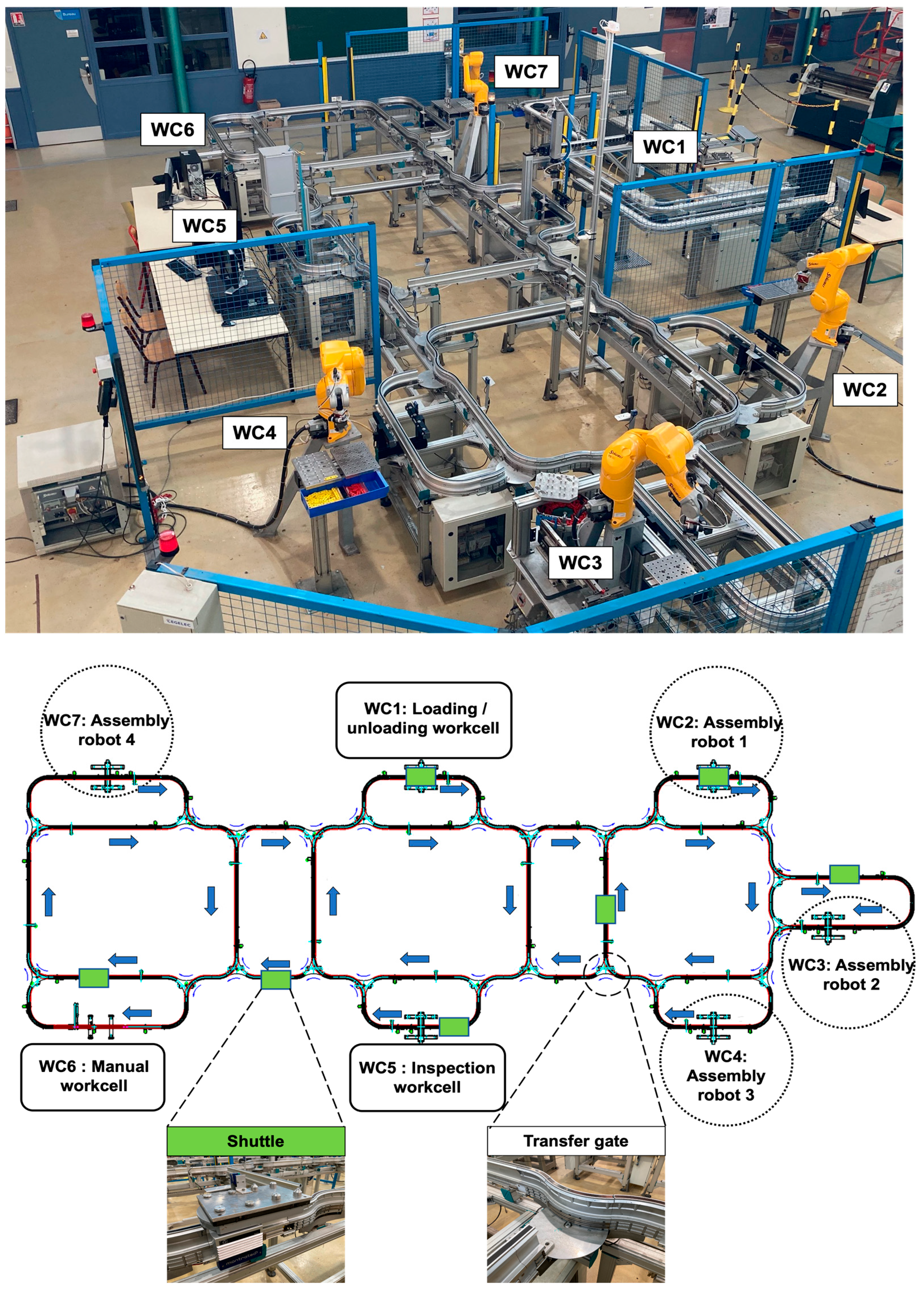
Before describing the proposed methodology, some assumptions are introduced, and an example of a FMS is given to clarify the different concepts used afterward.

3.1. Assumptions Relative to FMS Design

The FMS, considered in the present paper, is assumed to be composed of n processing CNC workcells. An example of such a FMS used at the Valenciennes S-mart pole [48] is depicted in Figure 1.

It is composed of seven workcells denoted WCi (i.e., a loading/unloading workcell, four robotized assembly workcells, an inspection workcell, and a manual workcell). The workcells are placed around a flexible transportation system based on Montratec technology [49]. This system is a monorail transport system using self-propelled shuttles to transport materials on tracks. As exhibited in Figure 1, transfer gates are used to connect physically the different tracks.

The shuttles can be programmed to follow a certain path based on the selected product. This enables rapid transitions for manufacturing different types of products. The whole FMS is monitored by a central control computer or SUP. All workcells, shuttles, and tracks are connected together wirelessly to the network using wireless switches except for the SUP, which is connected wired to the network through an Ethernet switch.

Each workcell follows the In-Loop Networked Control System (NCS) architecture [50]. It consists of sensors (S0, S1, …, Sx), a controller (K), and actuators (A0, A1, …, Ay). At the sensor nodes, the collected data are packaged and transmitted across the network to the controller K. The controller generates the appropriate control word based on the collected information from the sensors. This control word is then encapsulated and sent to the actuators via the network, which is the communication medium responsible for transferring the data among all the nodes. The actuators decapsulate the packets, and the control action is executed in the physical system.

The controller K is usually based on microcontrollers (MCUs). Some research proposed the utilization of FPGAs instead of MCUs for several reasons. In [51], FPGAs are described as programmable MCUs, where designers can combine several design components (processors with dedicated peripherals and customized computing hardware accelerators) on a single FPGA device platform. This results in simplifying design complexity and reducing the overall system cost. In comparison, reference [52] suggests the use of a System-on-Chip (SoC) FPGA device platform to allow the ability to offload the main processor by moving some of the processing tasks, such as control and communication tasks, inside the FPGA, as demonstrated in Figure 2.

Since FPGAs are reprogrammable, they can allow the adaptation of industrial designs to evolving industrial Ethernet protocols, IP improvements, and new hardware features within one FPGA on a common development platform. Moreover, the system can be enhanced according to the needs of the plant during runtime (upscaling or downscaling), as FPGAs allow I/O expansion at a lower cost and power compared to MCUs, Digital Signal Processing (DSP) blocks and Graphics Processing Units (GPUs) because they have limitations of performance in terms of throughputs and achievable bandwidth [9,10]. The use of FPGAs will increase a workcell’s life cycle and provide protection against hardware obsolescence through long FPGA life cycles and device migration to new FPGA families as opposed to MCUs, DSPs, and GPUs, which have a very limited lifetime [11]. Accordingly, in this research, the controller K will be implemented on a FPGA. In the system proposed next, it will be assumed that the application is simple, requiring mainly control actions; therefore, a Microblaze softcore processor (MicroBlaze; Xilinx, Inc.: San Jose, CA, USA) will be used.

3.2. Fault-Tolerant FMS Design

Given the harsh conditions of industrial environments, electromagnetic interference is very frequent, and the risk of faults arises in several ways, including sensor malfunctions, control systems failures, equipment damage, and actuator errors. Sensors can provide inaccurate readings or may fail entirely, while the controllers responsible for managing the manufacturing process can experience transient or permanent failures, thus affecting the overall operation. Moreover, the prolonged exposure of workcells to high levels of electromagnetic intrusions can damage the sensitive electronic components in the machinery. Accordingly, the design of a highly reliable FMS is proposed. The focus of this research will be on controller and/or SUP failures. Two levels of fault tolerance are introduced in the FMS: the workcell level and the system level.

At the workcell level, the fault model focuses on the faults that take place in the SRAM-based FPGA controller K, which include SEUs, SEFIs, and hard faults. SEUs in FPGAs are a significant concern, especially in harsh environments [53]. SEUs occur when a charged particle hits the FPGA, causing a bit flip in the configuration memory or user data. This can result in potential malfunctions or incorrect circuit behavior. Moreover, it can corrupt the data stored in registers or memory blocks in the FPGA, affecting calculations and data processing. SEUs can be mitigated by employing redundant modules and dynamically reconfiguring the affected areas of the FPGA by Dynamic Function eXchange (DFX) to enhance fault tolerance [54,55]. DFX refers to a capability that enables the dynamic reconfiguration of some functional modules within the FPGA while other modules still run normally [56]. It allows the FPGA to adapt to evolving requirements or operational conditions without the need to reconfigure the whole FPGA; as a result, the FPGA’s flexibility and efficiency are improved.

Unlike SEUs, which only affect individual bits, SEFIs induce a significant functional disruption, causing failure of the entire functionality of the FPGA because they occur in critical circuits involving Power-On-Reset (POR) circuitry, configuration port controllers (Joint Test Action Group (JTAG)), select-map communications ports, Internal Configuration Access Port (ICAP) controllers, reset nets and clock resources, as well as their associated control registers [13]. The control registers are responsible for executing all commands required for programming, reading, and checking the status of a FPGA device. They include general control registers, Cyclic Redundancy Check (CRC) registers for readback, Frame Address Registers, and watchdog circuitry. Accordingly, they disrupt the ability to perform readback from the FPGA, cause configuration bits to be written to an inaccurate frame address or cause a reset of the entire FPGA. SEFI detection is challenging since the affected blocks are not directly controlled by the user; as a result, the detection process is performed by external observation of abnormal behavior from the device. The only possible operation to recover from SEFIs is to switch off the FPGA and reconfigure the entire FPGA from the golden configuration memory [57].

Hard faults cause permanent failures within the FPGA fabric because they affect the silicon itself. They include Time-Dependent Dielectric Breakdown (TDDB), the hot-carrier effect, and electromigration [58]. TDDB is the phenomenon that occurs when the FPGA is subjected to high electric fields, which results in the breakdown of the insulating dielectric material in the FPGA over time. This may lead to the eventual failure of the affected Configurable Logic Blocks (CLBs) of the FPGA, causing operational errors or complete device malfunction, while the hot-carrier effect occurs when charge carriers (electrons or holes) gain high kinetic energy, which is also due to high electric fields within the semiconductor device, which leads to transistor aging, threshold voltage shifts, and increased leakage currents that degrade the FPGA’s performance and reliability. Electromigration takes place when metal atoms in conductive paths migrate as a result of high current densities, causing material degradation and eventual open or short circuits. Consequently, this may lead to FPGA interconnect failures.

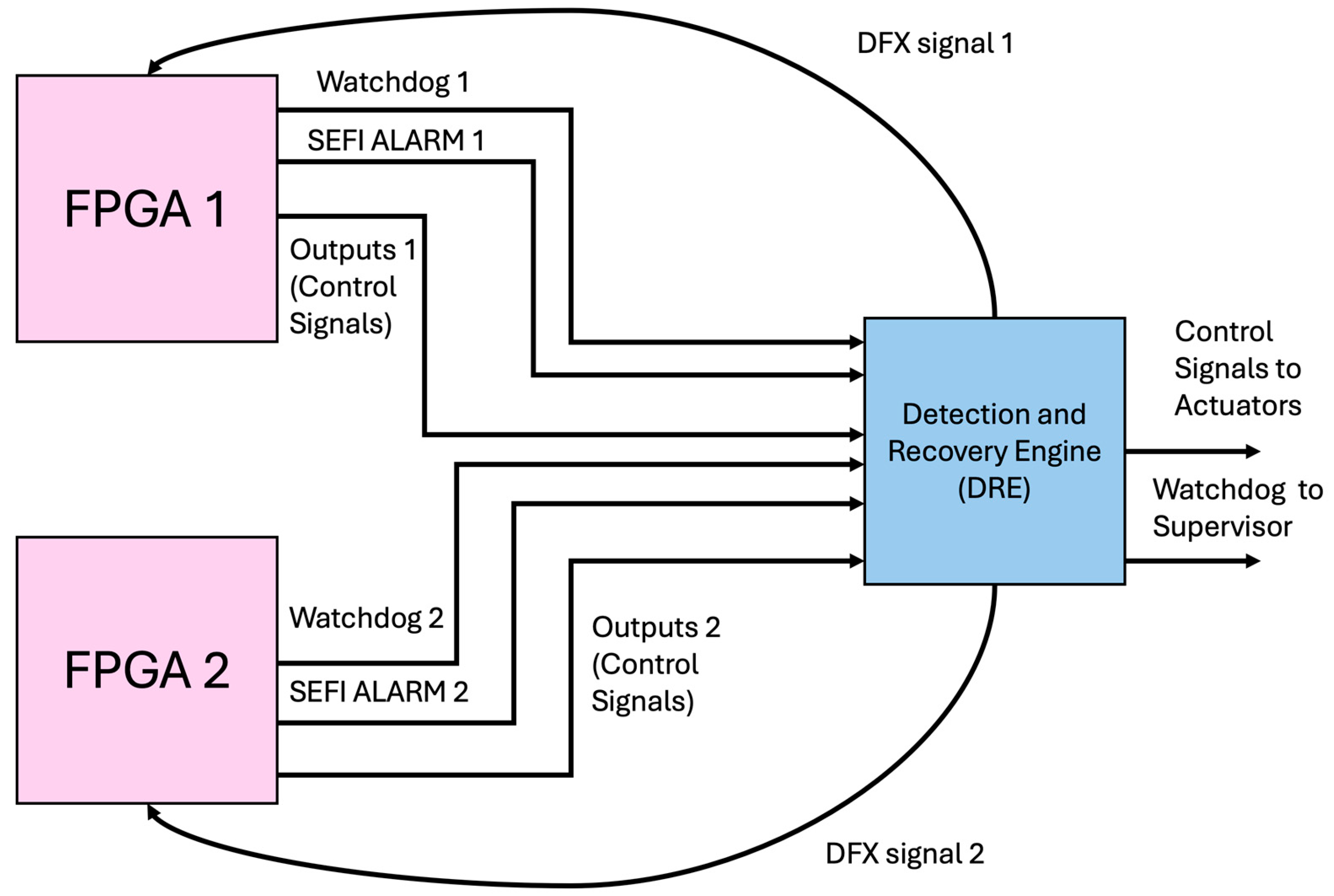
Addressing these reliability concerns is very critical in the FPGA design, requiring careful consideration and mitigation techniques to ensure the durability and reliability of the FPGA-based controllers. In this research, the redundancy approach, which will be applied to the FPGA-based controller in the workcell, is Duplication With Comparison (DWC) [14,59]. The proposed fault-tolerant design is composed of two identical FPGA-based controllers (FPGA1 and FPGA2) and a Detection and Recovery Engine (DRE) block, as shown in Figure 3. DFX signal 1 and DFX signal 2 represent the signals through which the recovery instructions are sent to FPGA1 and FPGA2.

The DRE block is responsible for SEU, SEFI, and hard fault detection. Then, if any fault is detected, it sends the appropriate recovery instructions to the faulty FPGA and delivers the control signals and the watchdog signal of the working controller to the actuators and the SUP, respectively. Each FPGA-based controller generates a watchdog signal and sends it to the DRE block along with the control signals (including the control action that should be sent to the actuators) and the SEFI alarm signal (indicating whether a SEFI event has occurred or not). For SEFI fault detection, the SEFI alarm signal is monitored by the DRE. If a SEFI exists, the DRE block orders the faulty FPGA to perform full reconfiguration of the FPGA. For SEUs and hard faults detection, the DRE block monitors the watchdog signals coming from the FPGA-based controllers and compares their control signals to check if they have identical values or not. If the control signals are not identical, this means that there is a SEU or a hard fault in one of the controllers. The faulty controller is identified by checking both watchdog signals. In this case, the DRE block orders the faulty controller to perform DFX and transmit the control signals from the active controller to the actuators. After completion of the DFX action, if the controller is still identified by the DRE as a faulty block, this means that a hard fault exists, and the system will continue working with the active controller only. If the active controller fails, the whole workcell will fail. However, if the faulty controller resumes operation, the system will function normally until the occurrence of another fault, upon which the same process will be repeated.

To test the robustness of the proposed architecture, the reliability of the fault-tolerant FPGA-based controller architecture is calculated using Stochastic Petri Nets (SPNs), and then it is compared to the reliability of the FPGA-based controller without applying any fault tolerance.

SPNs are widely used in the modeling and analysis of complex systems. SPNs permit the mathematical analysis of system functionality along with system reliability. They are composed of Place/Transition nets in which the place (p) represents the state of the system (denoted as p₁, p₂, …, p_n) while the transitions (t) refer to the changes that happen in the system (denoted as t₁, t₂, …, t_n) where these changes (firing events) occur after a random time. The distribution used for the interarrival time of the failures is usually the exponential distribution [14]. The exponential distribution is memoryless and is well-suited to describe the failure/firing events. Its hazard rate (or failure rate) is constant.

When a transition fires, a change in the state of the associated elements takes place. The tokens are the dots inside places that represent a specific configuration of the net. Once the network experiences a transition, the tokens move across the model from one place to another [60]. Markings (m) denoted as (m₁, m₂, …, m_m) represent the number of tokens in each place, while the firing rate (λ) is the rate of the exponential distribution associated with each transition. The SPN includes the following key components (P, T, F, K, W, M, and λ) [61], which are described with the required conditions as follows:

(1)

P = {p₁, p₂, …, p_n} is a limited set of places;

(2)

T = {t₁, t₂, …, t_n} is a limited set of transitions;

(3)

P ∪ T ≠ ∅ (means that the net is not empty);

(4)

P ∩ T ≠ ∅ (means that both are dual);

(5)

F ⊆ ((P × T) ∪ (T × P)) (means that the flow relationship is only between the elements of sets P and T);

(6)

dom (F) = {x|∃y: (x, y) ∈ F} (represents the set of the first element of the order couple contained in F);

(7)

cod (F) = {x|∃y: (y, x) ∈ F} (represents the set of the second element of the order couple contained in F);

(8)

dom (F) ∪ cod (F) = P ∪ T (means that there are no isolated elements);

(9)

N is a natural number, while N⁺ is a positive natural number;

(10)

K: P → N⁺ ∪ {∞} (represents the capacity function of the place);

(11)

W: F → N⁺ (represents the weight function of the directed arc);

(12)

M: P → N (represents the initial marking which should satisfy ∀_p ∈ P: M(p) ≤ K(p));

(13)

λ = {λ₁, λ₂, …, λ_n} (represents the set of transition firing rates).

Each transition follows an exponential distribution function with parameter λ_i [62]:

$$\forall t\in T:Ft=1-e^{-\lambda ix}$$

(1)

where λ_i is the average firing rate (λ_i > 0) and x is a variable (x ≥ 0). Moreover, the probability that two transitions will fire simultaneously is zero, and the reachable state graph of the SPN is isomorphic to a homogeneous Markov chain (MC), allowing it to be solved using Markov stochastic processes.

A Petri Nets model N can be represented as an incidence matrix [N] → ℤ, which is an integer matrix composed of |T| × |P| and indexed by T and P [63,64]. It describes the Petri Nets in mathematical form as follows:

$${\left[N\right]}_{\left|T\right|\times \left|P\right|}(t,p)=\left\{\begin{array}{c}W(t,p),(t,p)\in F\wedge (p,t)\notin F\\ -W(p,t),(t,p)\notin F\wedge (p,t)\in F\\ 0,\text{ otherwise}\end{array}\right.$$

(2)

The incidence matrix can be divided into the input matrix and output matrix:

Input matrix:

$${\left[N\right]}_{\left|T\right|\times \left|P\right|}^{+}(t,p)=\left\{{\left[N\right]}_{\left|T\right|\times \left|P\right|}\right(t,p\left)\right|\forall p,t\in N\}$$

(3)

Output matrix:

$${\left[N\right]}_{\left|T\right|\times \left|P\right|}^{-}(t,p)=\left\{{\left[N\right]}_{\left|T\right|\times \left|P\right|}\right(p,t\left)\right|\forall p,t\in \mathrm{N}\}$$

(4)

where $\left[N\right]$ = ${\left[N\right]}^{+}$ − ${\left[N\right]}^{-}$. Each negative element in $\left[N\right]$ or non-zero element in ${\left[N\right]}^{-}$ denotes one arc directed from place to transition.

The reliability of the system R(t) is the probability that the system remains in the operational state over time, which means that it can be calculated from the SPN as the probability that place F (representing the failure state) is empty at time t, where empty place indicates that it has no tokens. Let the number of places of the SPN be X. Let $P_i$(t) be the probability of being in place i at time t. Using the Chapman–Kolmogorov equations [14], the transient probability of being in any of the i places can be evaluated. P is the matrix, including the probabilities of each place i while T is the Transition Rate Matrix.

$${\displaystyle \frac{dP}{dt}}=P\times T$$

(5)

where

$${\displaystyle \frac{dP}{dt}}={\displaystyle \frac{d{P}_1}{dt}}\dots \dots \dots ..{\displaystyle \frac{d{P}_x}{dt}}$$

$$\mathrm{P}=[P_1\dots \dots ..P_X]$$

$$T_{ij}=\left\{\begin{array}{c}{\lambda }_{ij},\text{ if there is a transition from place }i\text{ to }j\\ -{\sum }_{k\ne i}{T}_{ik},\text{ if }i=j\text{ (diagonal elements)}\\ 0,\text{ otherwise (no direct transition)}\end{array}\right.$$

where ${\lambda }_{ij}$ is the rate of transition from place i to j

Let $P_1$(0) = 1, and all other places have an initial probability of zero. By substituting T and P in Equation (5), $P_i$(t) for each place i can be computed, and system reliability R(t) at time t can be obtained using Equation (6).

$$R\left(t\right)=1-P_F\left(t\right)$$

(6)

where $P_F\left(t\right)$ is the probability of being in the place in which the whole system fails.

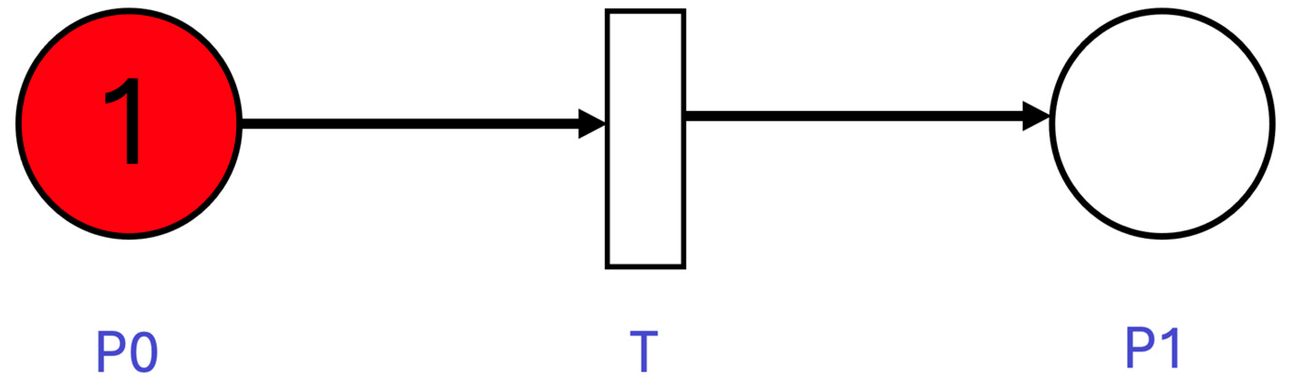
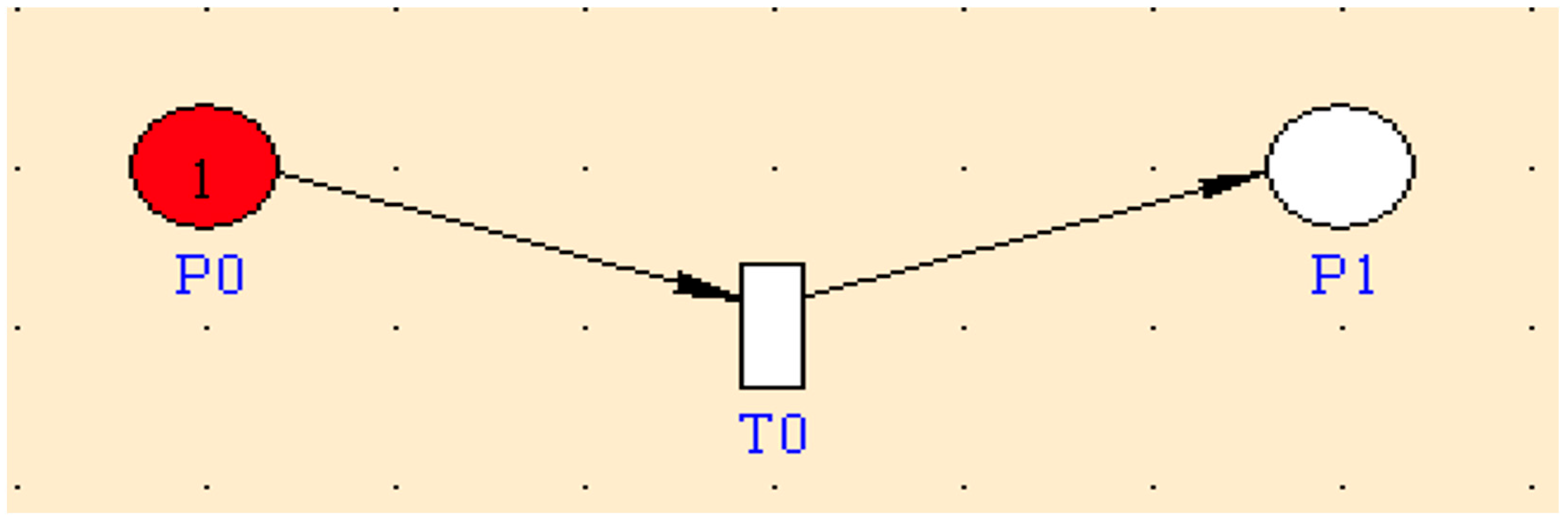
The reliability of the FPGA-based controller without applying the fault-tolerant technique is calculated using the SPN displayed in Figure 4.

Place P0 represents the fault-free state of the controller in which it works appropriately, and it contains 1 token, which shows that the system is initially in this place. If the controller is hit by a SEU, hard fault, or SEFI, with a rate of (SEU + HARD + SEFI), the token will move to place P1, which represents the failure of the controller through transition T0. The SEU is the SEU failure rate of the FPGA-based controller, which is calculated based on the SEU failure rate per bit and the size of the bit file of the controller. While HARD is the hard fault rate of the FPGA-based controller and SEFI is the SEFI rate of the controller. The reliability of the system is calculated as the probability that place P1 (representing the failure state) is empty at time t. The incidence matrix of the model is shown in the following equation:

$$\begin{array}{r}\mathrm{P}0\mathrm{P}1\\ {\left[N\right]}_{\left|T\right|\times \left|P\right|}=\mathrm{T}\left[\begin{array}{cc}-1& 1\end{array}\right]\end{array}$$

(7)

The reliability of the FPGA-based controller without applying the fault-tolerant technique $R_S$(t) is calculated as follows:

$$R_S\left(t\right)=1-P_{\mathrm{P}1}\left(t\right)$$

(8)

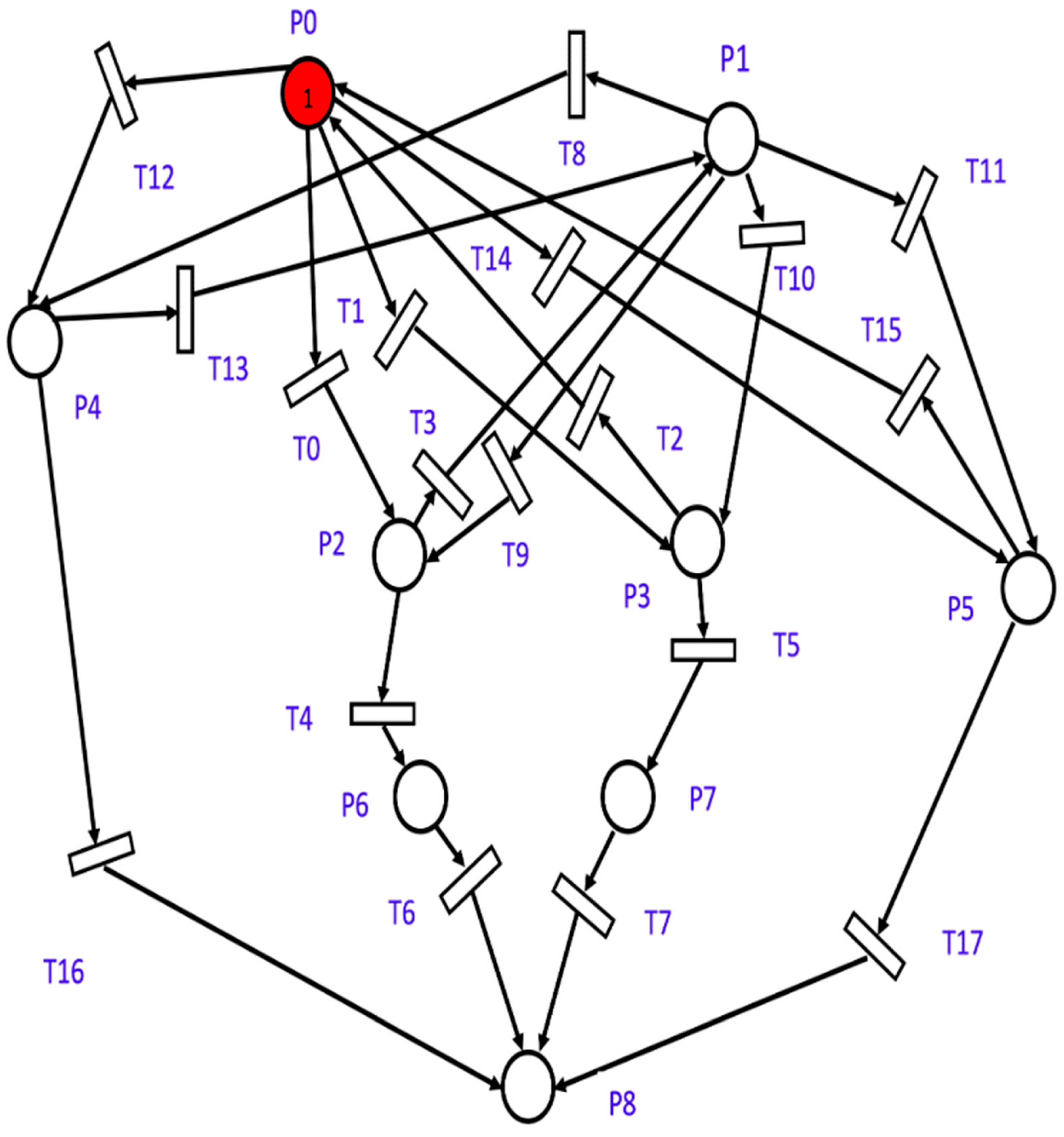
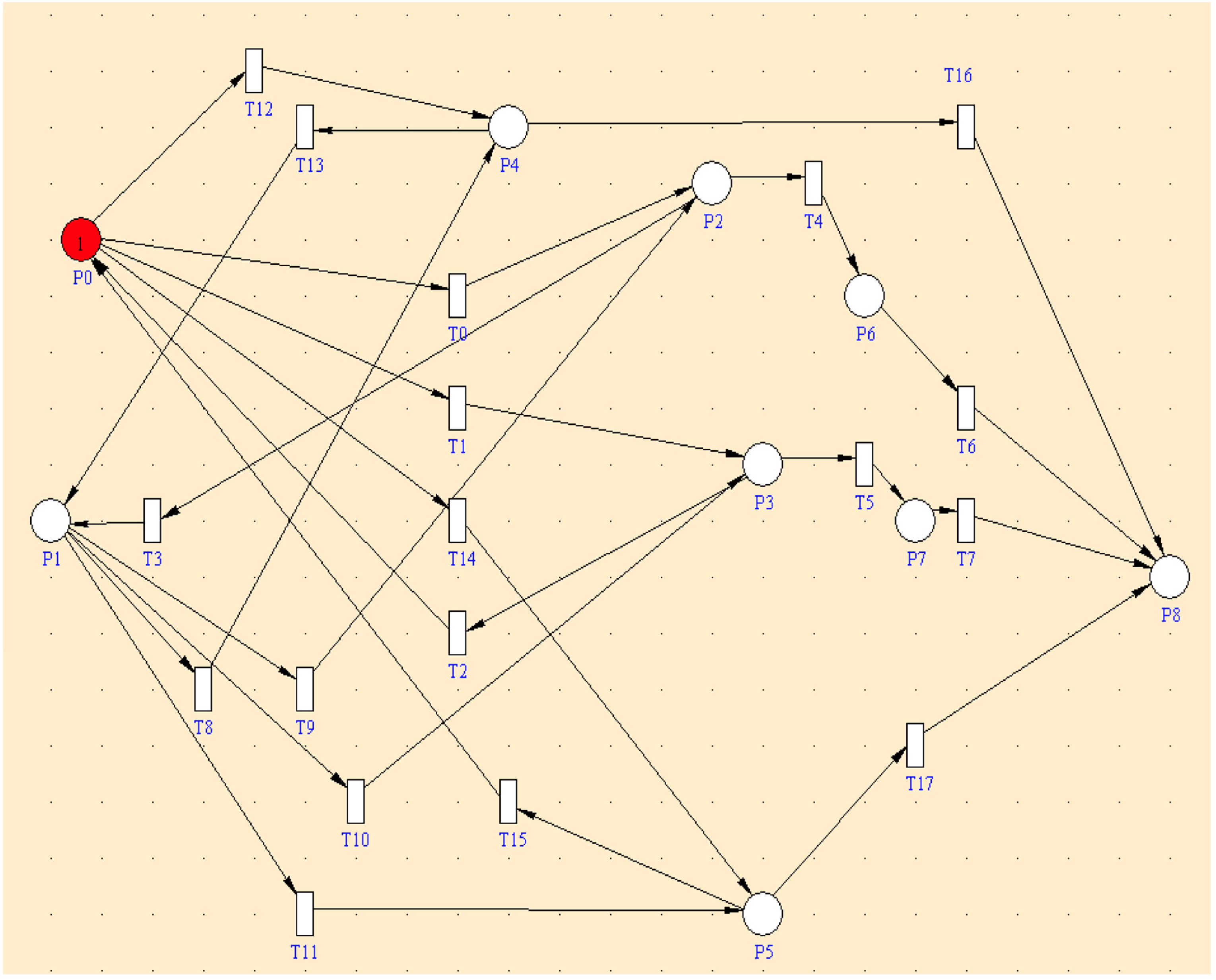
The proposed fault-tolerant FPGA-based controller can be described using nine places (states) and eighteen transitions in the SPN, which are described in

Table 2. Places of fault-tolerant FPGA-based controller SPNs.

Place	Description
P0	M1 and M2 are in a fault-free state. DRE transmits the control signals from the M1 controller to the actuators.
P1	M1 and M2 are in a fault-free state. DRE transmits the control signals from the M2 controller to the actuators.
P2	SEU or hard fault detected in M1. DRE orders M1 to perform DFX. The control signals are transmitted from M2 to the actuators.
P3	SEU or hard fault detected in M2. DRE orders M2 to perform DFX. The control signals are transmitted from M1 to the actuators.
P4	SEFI detected in M1. DRE orders M1 to perform full reconfiguration. The control signals are transmitted from M2 to the actuators.
P5	SEFI detected in M2. DRE orders M2 to perform full reconfiguration. The control signals are transmitted from M1 to the actuators.
P6	Hard fault detected in M1. System will proceed to function with M2 only.
P7	Hard fault detected in M2. System will proceed to function with M1 only.
P8	The whole system fails.

and

Table 3. Transitions of fault-tolerant FPGA-based controller SPNs.

Transition	Rate
T0	SEU_M1 + HARD_M1
T1	SEU_M2 + HARD_M2
T2	Z * U
T3	Z * U
T4	(1 − Z) * U
T5	(1 − Z) * U
T6	SEU_M2 + HARD_M2 + SEFI_M2
T7	SEU_M1 + HARD_M1 + SEFI_M1
T8	SEFI_M1
T9	SEU_M1 + HARD_M1
T10	SEU_M2 + HARD_M2
T11	SEFI_M2
T12	SEFI_M1
T13	USEFI_M1
T14	SEFI_M2
T15	USEFI_M2
T16	SEU_M1 + HARD_M1 + SEFI_M1 + SEU_M2+ HARD_M2 + SEFI_M2
T17	SEU_M1 + HARD_M1 + SEFI_M1 + SEU_M2+ HARD_M2 + SEFI_M2

. Assume that M1 and M2 are the two identical FPGA-based controllers, and the failure rates of the SEU, hard faults, and SEFI of M1 are SEU_M1, HARD_M1, and SEFI_M1, respectively. For M2, the failure rates for the SEU, hard faults, and SEFI are represented by SEU_M2, HARD_M2, and SEFI_M2. The model is based on the occurrence of a single fault at any given time.

The incidence matrix of the model is presented in the following equation:

$$\begin{array}{ccc}{\left[N\right]}_{\left|T\right|\times \left|P\right|}=& & \begin{array}{ccccccccc}\mathrm{P}0& \mathrm{P}1& \mathrm{P}2& \mathrm{P}3& \mathrm{P}4& \mathrm{P}5& \mathrm{P}6& \mathrm{P}7& \mathrm{P}8\end{array}\\ & \begin{array}{c}\mathrm{T}0\\ \mathrm{T}1\\ \mathrm{T}2\\ \mathrm{T}3\\ \mathrm{T}4\\ \mathrm{T}5\\ \mathrm{T}6\\ \mathrm{T}7\\ \mathrm{T}8\\ \mathrm{T}9\\ \mathrm{T}10\\ \mathrm{T}11\\ \mathrm{T}12\\ \mathrm{T}13\\ \mathrm{T}14\\ \mathrm{T}15\\ \mathrm{T}16\\ \mathrm{T}17\end{array}& \begin{array}{c}\left[\begin{array}{ccccccccc}-1& 0& 1& 0& 0& 0& 0& 0& 0\\ -1& 0& 0& 1& 0& 0& 0& 0& 0\\ 1& 0& 0& -1& 0& 0& 0& 0& 0\\ 0& 1& -1& 0& 0& 0& 0& 0& 0\\ 0& 0& -1& 0& 0& 0& 1& 0& 0\\ 0& 0& 0& -1& 0& 0& 0& 1& 0\\ 0& 0& 0& 0& 0& 0& -1& 0& 1\\ 0& 0& 0& 0& 0& 0& 0& -1& 1\\ 0& -1& 0& 0& 1& 0& 0& 0& 0\\ 0& -1& 1& 0& 0& 0& 0& 0& 0\\ 0& -1& 0& 1& 0& 0& 0& 0& 0\\ 0& -1& 0& 0& 0& 1& 0& 0& 0\\ -1& 0& 0& 0& 1& 0& 0& 0& 0\\ 0& 1& 0& 0& -1& 0& 0& 0& 0\\ -1& 0& 0& 0& 0& 1& 0& 0& 0\\ 1& 0& 0& 0& 0& -1& 0& 0& 0\\ 0& 0& 0& 0& -1& 0& 0& 0& 1\\ 0& 0& 0& 0& 0& -1& 0& 0& 1\end{array}\right]\end{array}\end{array}$$

(9)

Initially, the system resides in place P0, marked by one token, as shown in Figure 5. When a transition occurs in the network, the token transfers from one place to another within the model. If M1 becomes faulty due to a SEU or a hard fault, the system moves to place P2 through transition T0 with the rate of SEU_M1 + HARD_M1. In this place, the DRE block orders M1 to perform DFX and transmits the control signals from M2 to the actuators. Following the completion of the DFX, if the controller becomes online, the system will transfer to place P1 through transition T3 with a rate of Z * U, where Z is the conditional probability that the fault is a SEU. The relative frequency of a SEU versus hard failures is a crucial factor in the calculation of Z. Furthermore, assume that the time taken to reconfigure the controller (BIT file over the network) is exponentially distributed with an expected value of 1/U. Consequently, the repair rate is given by U. In the case that the DRE still identifies the controller as a faulty block, it signifies the existence of a hard fault, and the system will proceed to function with M2. This means that the system will move to place P6 through transition T4 with the rate of (1 − Z) * U. If M2 becomes defective, the whole system will fail, and this indicates that the system will move to place P8 via transition T6 at a rate of SEU_M2 + HARD_M2 + SEFI_M2.

If a SEFI is detected in M1, the DRE block instructs the faulty FPGA M1 to initiate a full reconfiguration process, and the system will continue working with M2; accordingly, the system will move from place P0 to place P4 through transition T12 with a rate of SEFI_M1. If M1 becomes online, the system will move to place P1 through T13 via rate USEFI_M1, which is the repair rate of M1 due to the SEFI fault. If any other fault exists, the entire system will fail, which means that the system will move to place P8 through transition T16 with a rate of SEU_M1 + HARD_M1 + SEFI_M1 + SEU_M2 + HARD_M2 + SEFI_M2.

Similarly, if the system is in place P0 and M2 becomes faulty due to a SEU or hard fault, the system transitions to place P3 through transition T1 at the rate of SEU_M2 + HARD_M2. In this state, the DRE orders M2 to perform DFX while M1 transmits control signals. If M2 becomes online after DFX, the system transitions to place P0 through transition T2 at the rate of Z * U. If M2 remains faulty, indicating a hard fault, the system moves to place P7 through transition T5 at the rate of (1 − Z) * U.

In the event that M1 becomes defective, the entire system will fail, leading to a transition to place P8 via transition T7 at a rate of SEU_M1 + HARD_M1 + SEFI_M1. If SEFI is detected in M2, the DRE commands a full reconfiguration, and the system moves to place P5 through transition T14 at the rate of SEFI_M2. If M2 becomes online, the system transitions to place P0 via T15 at the repair rate USEFI_M2. When any other fault leading to system failure occurs, the transfer to place P8 through transition T17 at the rate of SEU_M1 + HARD_M1 + SEFI_M1 + SEU_M2 + HARD_M2 + SEFI_M2 takes place. When the system is in P1 and M2 is hit by a SEU or a hard fault, the system transitions to place P3 through transition T10 at the rate of SEU_M2 + HARD_M2. Conversely, if M1 is struck by a SEU or a hard fault, the system transitions to place P2 through transition T9 at the rate of SEU_M1 + HARD_M1.

Upon detection of a SEFI in M1, the system transitions to place P4 through transition T8 at the rate of SEFI_M1. On the other hand, if a SEFI is detected in M2, the system moves to place P5 through transition T11 at the rate of SEFI_M2. Then, the model proceeds as previously described.

The reliability of the proposed fault-tolerant FPGA-based controller is calculated as the probability that place P8 (representing the failure state) is empty at time t. The SPN of the proposed fault-tolerant FPGA-based controller is composed of 9 places. Let $P_i$(t) be the probability of being in place i (where i ∈ {P0, P1, P2, P3, P4, P5, P6, P7, P8}) at time t. Using the Chapman–Kolmogorov equations [14] and assuming $P_{\mathrm{P}0}$ (0) = 1 while $P_{\mathrm{P}1}$ (0) = $P_{\mathrm{P}2}$ (0) = $P_{\mathrm{P}3}$ (0) = $P_{\mathrm{P}4}$ (0) = $P_{\mathrm{P}5}$ (0) = $P_{\mathrm{P}6}$ (0) = $P_{\mathrm{P}7}$ (0) = $P_{\mathrm{P}8}$ (0) = 0, the transient probability of residing in any of the i places can be evaluated as follows:

$${\displaystyle \frac{d{P}_{ps}}{dt}}=P_{ps}\times T_{Ps}$$

(10)

where

$${\displaystyle \frac{d{P}_{ps}}{dt}}={\displaystyle \frac{d{P}_{\mathrm{P}0}}{dt}}\dots \dots \dots ..{\displaystyle \frac{d{P}_{\mathrm{P}8}}{dt}}$$

$$P_{ps}=[P_{\mathrm{P}0}{P}_{\mathrm{P}1}{P}_{\mathrm{P}2}{P}_{\mathrm{P}3}{P}_{\mathrm{P}4}{P}_{\mathrm{P}5}{P}_{\mathrm{P}6}{P}_{\mathrm{P}7}{P}_{\mathrm{P}8}]$$

$$T_{Ps}=\left[\begin{array}{cccccccc}(-\mathrm{T}0-\mathrm{T}1-\mathrm{T}12-\mathrm{T}14)& 0& \mathrm{T}0& \mathrm{T}1& \dots & 0& 0& 0\\ 0& (-\mathrm{T}9-\mathrm{T}10-\mathrm{T}8-\mathrm{T}11)& \mathrm{T}9& \mathrm{T}10& \dots & 0& 0& 0\\ 0& \mathrm{T}3& (-\mathrm{T}3-\mathrm{T}4)& 0& \dots & \mathrm{T}4& 0& 0\\ \mathrm{T}2& 0& 0& (-\mathrm{T}2-\mathrm{T}5)& \dots & 0& \mathrm{T}5& 0\\ 0& \mathrm{T}13& 0& 0& \dots & 0& 0& \mathrm{T}16\\ \mathrm{T}15& 0& 0& 0& \dots & 0& 0& \mathrm{T}17\\ 0& 0& 0& 0& \dots & -\mathrm{T}6& 0& \mathrm{T}6\\ 0& 0& 0& 0& \dots & 0& -\mathrm{T}7& \mathrm{T}7\\ 0& 0& 0& 0& \dots & 0& 0& 0\end{array}\right]$$

The reliability of the proposed fault-tolerant FPGA-based controller technique $R_{PS}$(t) is calculated as follows:

$$R_{PS}\left(t\right)=1-P_{\mathrm{P}8}\left(t\right)$$

(11)

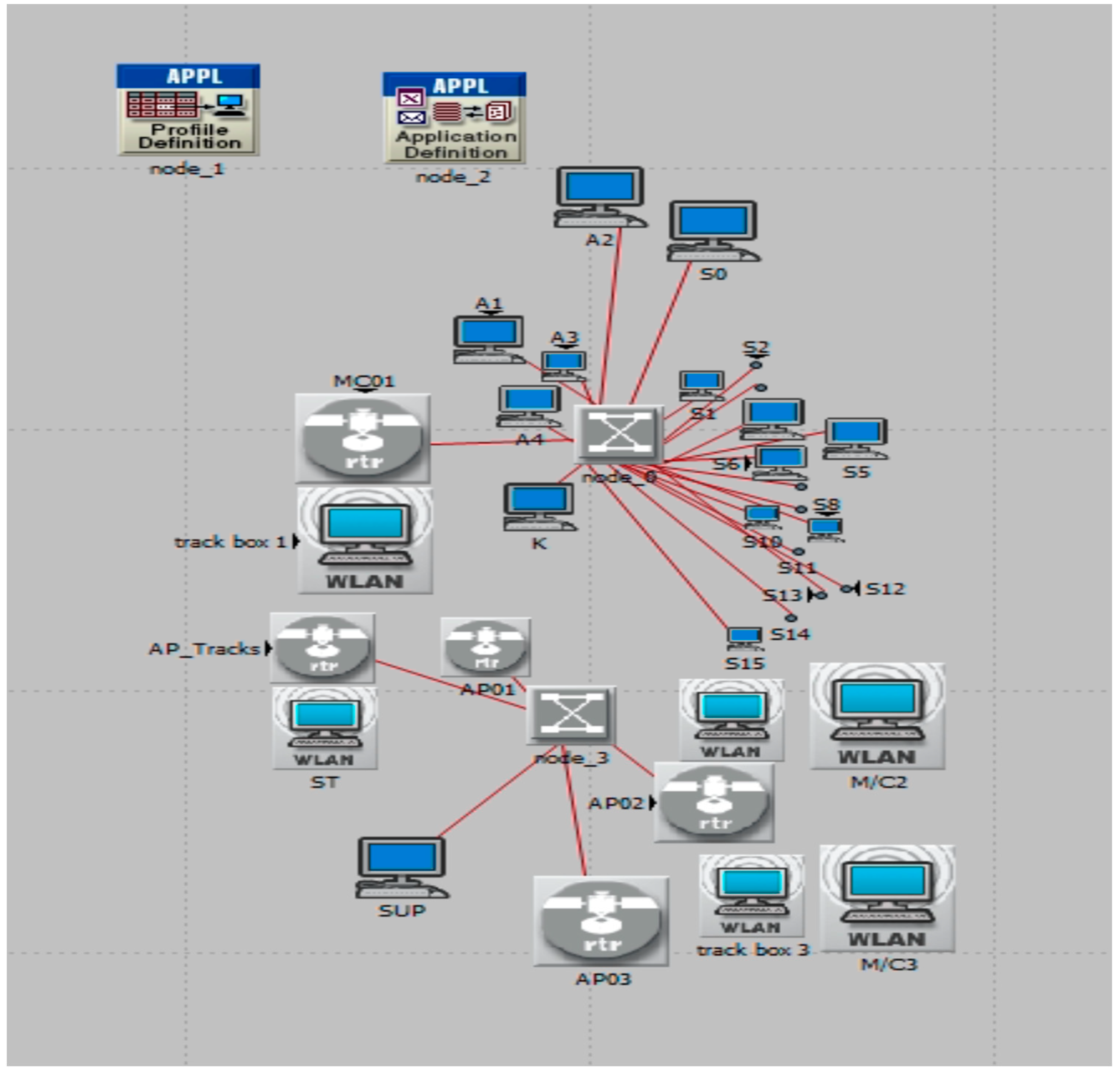
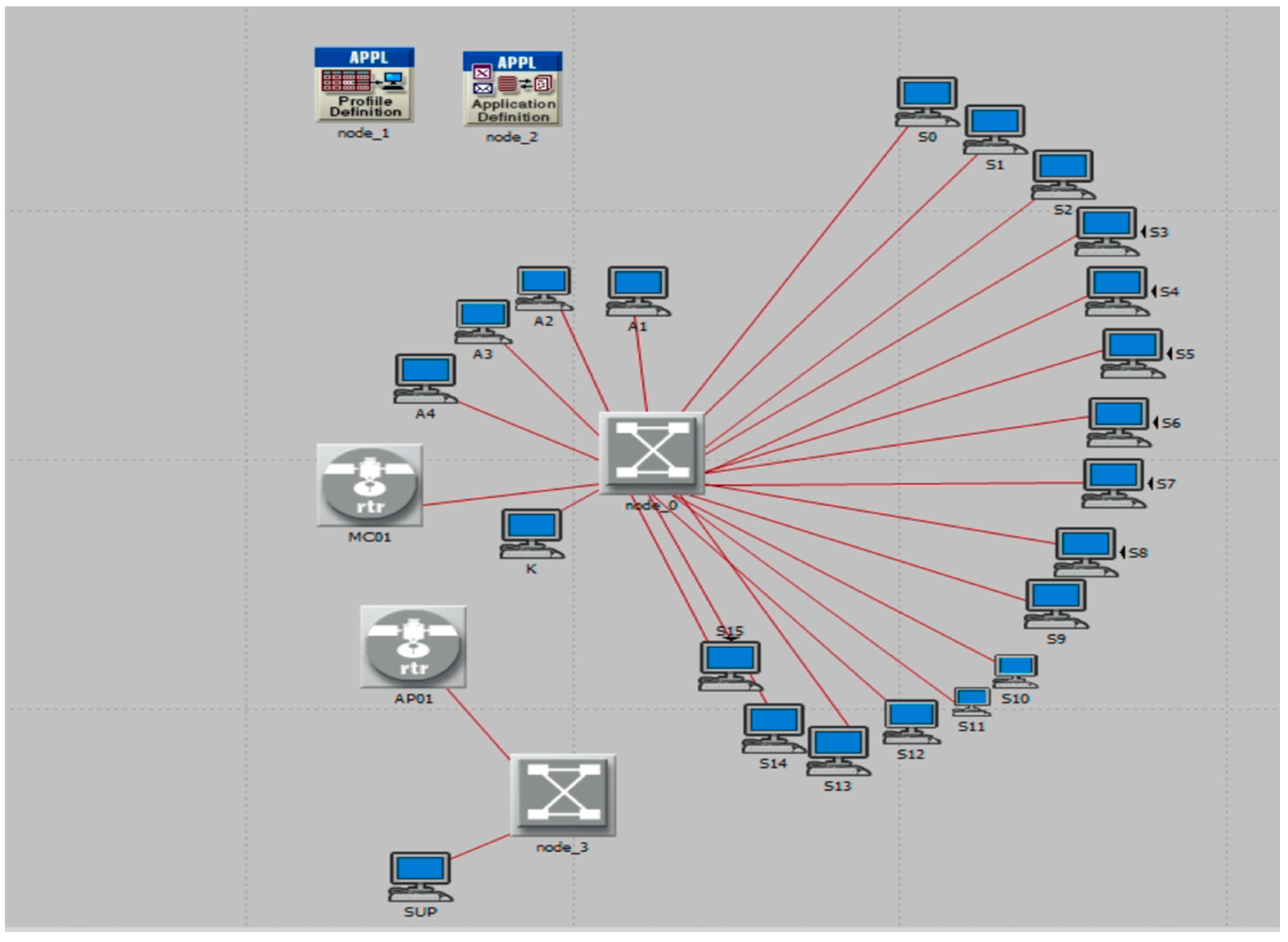
The role of fault tolerance at the system level becomes obvious when the fault-tolerant FPGA-based controller fails. Under normal conditions, the SUP continuously receives a watchdog signal from the workcell’s controller. However, when the controller becomes faulty, the SUP replaces it. Consequently, all the sensor and actuator signals that were initially sent to the faulty controller are rerouted directly to the SUP. The evaluation of network performance is based on end-to-end delays. The system is modeled and simulated using the Riverbed Network Modeler [16] in both fault-free and fault-tolerant scenarios. Studying normal conditions is crucial to ensure that the system operates correctly in the absence of faults.

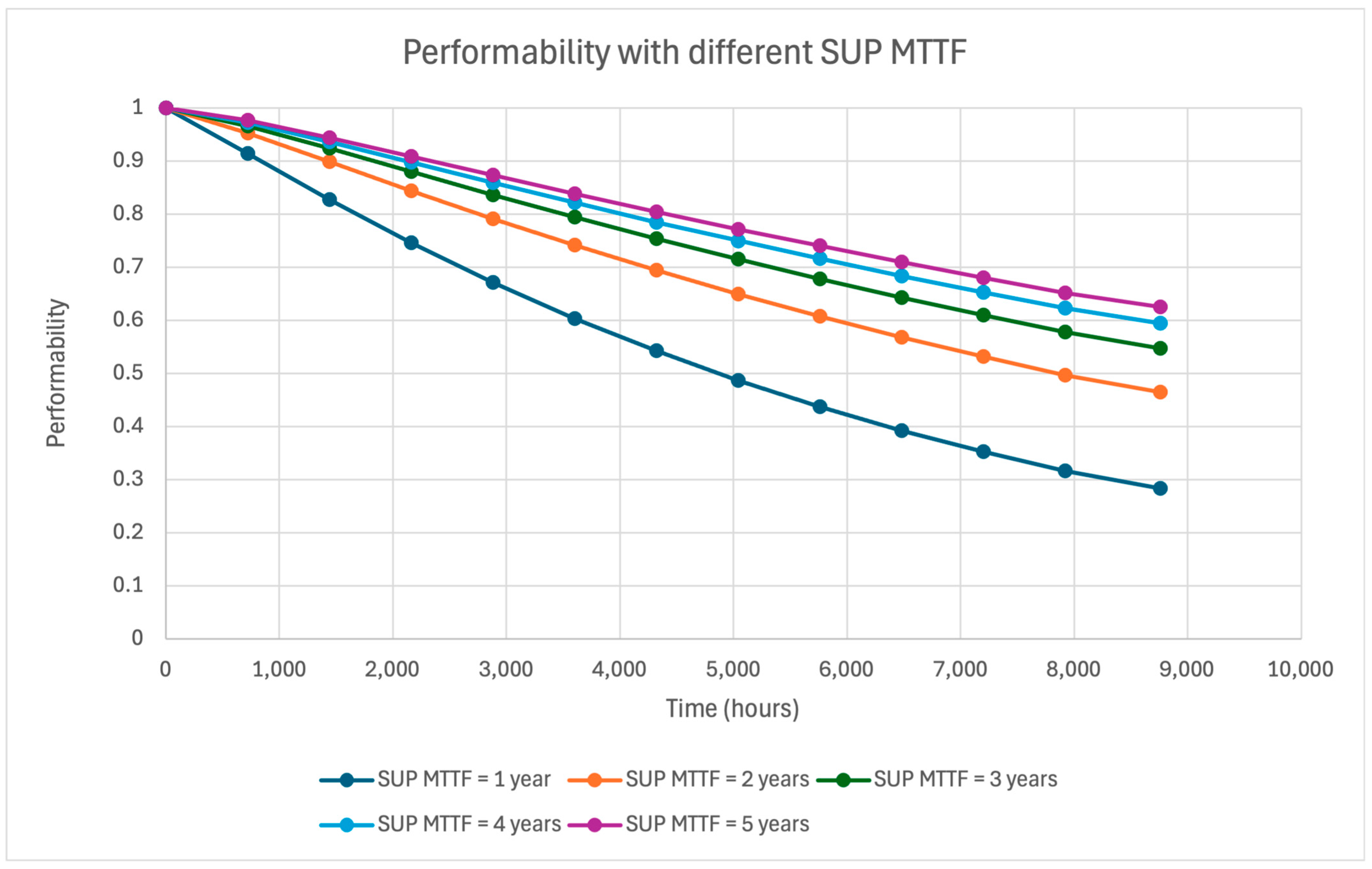
If the system is tested and shows increased delays due to network congestion, the solution is to reduce the workcell’s speed, bringing the network delay back within acceptable limits. To ensure that the system meets performance expectations despite reduced speeds resulting from a workcell failure, a performability analysis is conducted. Given that the analysis is time-dependent, the transient probabilities of the system being in each state over time will be considered, and the Transient Performability (TP) will be subsequently calculated.

TP is a metric used to assess a system’s performance during a temporary period of operation or transition, particularly when it is exposed to varying conditions or failures. It examines the system’s capability to maintain its operational performance or functionality during non-steady-state conditions, such as failure existence. The TP(t) is obtained as follows [65]:

$$TP\left(t\right)=\sum _{i\in \psi }{P}_i{Rew}_i$$

(12)

where ψ is the set of states of the system model, $P_i$(t) is the probability of residing in state i at time t, and Rew_i is the reward/penalty of each state i. The metric used as the penalty is the operational speed of the workcells in state i. The calculation of TP begins with identifying the system’s operational and failure states and then determining the probability of the system being in each state at a given time t. Subsequently, a penalty will be associated with each state to reflect the system’s performance in that state. The penalty (operational speed of the workcells) is determined based on the simulations conducted for each state using Riverbed Network Modeler (Riverbed Network Modeler; Riverbed Technology, Inc.: San Francisco, CA, USA) [16]. Then, the performability is determined by summing the products of each state’s penalty and the probability that the system will be in that state at a given time. TP can be derived from the system’s reliability in operational states, as reliability functions provide the probability of the system being in an operational state. Therefore, $P_i$(t), which is the probability of the system being in state i at time t, can be calculated based on the product of the reliability of the workcells in state i at that time t. In the following section, a case study is presented to rigorously evaluate and validate the proposed methodology. This analysis aims to assess the methodology’s applicability and effectiveness in a real-world context.

4. Case Study

In this case study, the design and implementation of a fault-tolerant FMS are investigated to test the ability of the system to enhance operational efficiency and ensure resilience in production through multiple levels of fault tolerance. As previously stated, fault tolerance in a FMS is implemented at two levels: the workcell level and the system level. Note that this case study represents “a proof of concept” approach to the solution of the problem.

4.1. Fault Tolerance at Workcell Level

At the workcell level, the proposed fault-tolerant FPGA-based controller architecture consists of two identical FPGA-based controllers integrated with a DRE module. The prototype is implemented using two Zybo Z7-20 AMD boards [66], representing the two duplicate FPGA-based controllers, while the Arduino DUE development board serves as the DRE module, as shown in Figure 6.

The FPGA-based controller of the workcell is represented by a 32-bit MicroBlaze softcore, which is sufficient for the specific requirements of the system under study (control tasks only). Each FPGA-based controller communicates serially with the DRE module, represented by an Arduino DUE, using the Universal Asynchronous Receiver-Transmitter (UART). Therefore, the Advanced eXtensible Interface (AXI) UART Lite interface is added to the MicroBlaze. Through this connection, the watchdog and SEFI alarm signals are sent to the DRE, and the DFX signal is sent back to the FPGA-based controller. Control signals are delivered to the DRE using general purpose Input/Output (GPIO) pins, as shown in the MicroBlaze block diagram in Figure 7.

The design is synthesized and implemented on the Zybo (Z7-20) AMD board using Xilinx’s Vivado design suite. The resource utilization includes 1726 Slice LUTs, 1467 Slice Registers, 32 BRAMs, and 3 DSPs, while the power consumption is 0.241 W. The Controller Bitstream size is 3951 KB.

Three experiments were conducted to demonstrate the system’s behavior in case of the occurrence of a SEFI, SEU, or hard fault. This is done by using the PuTTY terminal, which displays the UART communication between the two FPGAs and the DRE. When the UART communication is initiated, each FPGA sends the following statement “Starting UART watchdog = Alive” to the DRE to indicate that the UART interface has been successfully started and the watchdog mechanism is operational. Then, each FPGA sends the outputs (control signals) and SEFI alarm signals to the DRE. Based on these signals, the DRE detects whether a SEFI, SEU, or hard fault exists, and the system takes the appropriate action for each case. If the watchdog signal is not received, the FPGA is considered to be non-operational.

The first experiment investigates the system’s behavior in case a SEFI occurs. The SEFI alarm signal is represented by 1 bit: logic ‘0’ represents that no SEFI exists, and logic ‘1’ represents that SEFI exists. If a SEFI is detected, the DRE block instructs the faulty FPGA to undergo a full reconfiguration for the whole board.

The second experiment examines the system’s behavior in the presence of a SEU. The watchdog signal is represented as a string: “Alive” indicates that no SEU is present, while “Dead” signifies that aa SEU exists. Additionally, the DRE module compares the control signals from both FPGA-based controllers. If aa SEU is detected, the DRE block instructs the faulty controller to execute DFX (MicroBlaze processor) and transmits the control signals from the active controller to the actuators.

The third experiment evaluates the system’s behavior in the presence of a hard fault. If the DRE identifies the controller as faulty after the DFX action has been completed in response to a SEU, this confirms the existence of a hard fault. Consequently, the system will operate exclusively with the active controller.

Several scenarios are being explored, each with varying system parameters, to examine the impact on system reliability under different conditions and system parameters. Using SPNs, the first scenario investigates the difference in reliability over time between the fault-tolerant FPGA-based controller and the corresponding simplex FPGA-based controller without any fault tolerance.

Table 4. Key parameter values in SPNs.

Parameter	Value
SEU	0.027/day
SEU_M1	0.027/day
SEU_M2	0.027/day
HARD	0.000135/day
HARD_M1	0.000135/day
HARD_M2	0.000135/day
U	125,947.52/day
SEFI	4.5 × 10−4 upset/device/day
SEFI_M1	4.5 × 10−4 upset/device/day
SEFI_M2	4.5 × 10−4 upset/device/day
USEFI_M1	61,714.285/day
USEFI_M2	61,714.285/day

includes all the parameters required for the SPNs. Note that the parameters related to a SEU are computed based on a SEU failure rate per bit = 1 × 10⁻⁸/day [67], and the SEFI failure rate is adopted directly from the data reported in [68].

The Stochastic Petri Net models for both the standard FPGA-based controller (without fault tolerance) and the proposed fault-tolerant FPGA-based controller are implemented in SHARPE [15], as shown in Figure 8 and Figure 9, respectively.

Table 5. Scenario 1, proposed system vs. simplex system reliability.

Time (Hours)	Simplex System (%)	Proposed System (%)
0	100	100
720	43.711892	95.08161
1440	19.107295	85.21352
2160	8.35216	74.34146
2880	3.6508871	64.01595
3600	1.5958718	54.7667
4320	0.6975858	46.69943
5040	0.3049279	39.75347
5760	0.1332898	33.81143
6480	0.0582635	28.74482
7200	0.0254681	24.43188
7920	0.0111326	20.76363
8760	0.0048663	17.64507

demonstrates the reliability difference between the two models. As expected, the proposed fault-tolerant FPGA-based controller consistently outperforms the standard system in terms of reliability over time.

The second scenario focused on studying the effect of the Z parameter, which reflects the conditional probability that a fault was transient and the system successfully restored the repaired controller to normal operation, on the reliability of the proposed fault-tolerant FPGA-based controller. While this parameter impacts the reliability of the proposed system, it has no effect on the simplex system due to its lack of fault tolerance. A higher Z value corresponds to a greater likelihood of recovering from a transient failure.

Table 6. Scenario 2, proposed system reliability for different values of Z.

Time (Hours)	Z = 0.8	Z = 0.90	Z = 0.95	Z = 0.97	Z = 0.99	Z = 0.999
0	100	100	100	100	100	100
720	90.69437	95.08161	97.4702	98.4646	99.482	99.948
1440	75.69319	85.21352	92.1615	95.1835	98.355	99.8337
2160	56.65516	74.34146	85.9668	91.2636	96.977	99.6925
2880	42.45355	64.01595	79.6876	87.183	95.502	99.5395
3600	31.32976	54.7667	73.6507	83.145	94	99.3816
4320	22.9176	46.69943	67.9771	79.2331	92.499	99.2217
5040	16.67729	39.75347	62.6996	75.4787	91.013	99.0611
5760	12.0987	33.81143	57.8138	71.8905	89.547	98.9003
6480	8.760865	28.74482	53.301	68.4679	88.102	98.7395
7200	6.336813	24.43188	49.137	65.2059	86.68	98.5789
7920	4.580391	20.76363	45.2969	62.0984	85.281	98.4186
8760	3.309465	17.64507	41.7562	59.1386	83.903	98.2585

shows the reliability of the proposed system for different Z values over time calculated using Matlab.

Table 6 shows the reliability of the proposed system for different values of Z, employing the same failure and repair rates as in scenario 1. The results indicate that Z plays a critical role in the system’s reliability over time. As Z increases, the system’s capacity to recover from transient failures improves through the implementation of DFX, leading to a considerable enhancement in both system reliability and the potential mission duration. It is important to highlight that the Z parameter is influenced not only by the ratio of transient to permanent failures but also by the likelihood of successful reconfiguration and reintegration of the repaired controller. As a result, the proposed system is well-suited for harsh industrial or factory-floor environments, where transient failures are more frequent than permanent ones.

4.2. Fault Tolerance at System Level

The fault-tolerant FMS under study comprises three CNC processing workcells, a shuttle for material transport, and a network of connected tracks. It corresponds to the right part of the FMS depicted in Figure 1 with three robotized assembly workcells (denoted WC2, WC3, and WC4). The central SUP controls the entire system via a wired connection, while the shuttle, CNC workcells, and tracks communicate wirelessly. Figure 10 shows the simulated model of the cell using Riverbed [16].

Each workcell utilizes the In-Loop Networked Control System (NCS) framework, which is composed of 16 sensors (S0, S1, …, S15), a controller (K), and four actuators (A0, A1, A2, and A3) linked in a star topology using an Ethernet switch, as shown in Figure 11. The workcell operates at a rotational speed of 1 revolution per second. Consequently, the sampling period is 694 µs, utilizing a 1440-pulse electric encoder for a full rotation of 360 mechanical degrees. Figure 11 shows the simulated model of the FMS using Riverbed [16].

The scenarios simulated are the fault-free scenario and the one with a failure of one of the workcell controllers.

4.2.1. Fault-Free Scenario

The first scenario represents a system operating under normal conditions, where all nodes are functioning as expected. During this phase, all workcells in the FMS are fully active, and watchdog packets are continuously exchanged between each workcell and the SUP. Moreover, each workcell operates at a rotational speed of 1 revolution per second (full speed), which means that the sampling period (packet delivery deadline) equals 694 µs. Using Riverbed Modeler [16], the model is verified. The simulations show that the system satisfies the control deadline requirements, with total end-to-end delays remaining within a single sampling period and no packet loss occurring.

4.2.2. Failure of One Workcell Controller

The second scenario involved the controller failure in one workcell. In this case, the SUP takes over, and all sensor and actuator signals originally connected to the faulty controller are redirected to it. The system is tested but the simulation shows obvious violation in the total end-to-end delays as a result of network congestion. The proposed solution is to decrease the workcell’s speed by half to a rotational speed of 0.5 revolutions per second, which means that the sampling period (packet delivery deadline) equals 1440 µs, thereby reducing network congestion and bringing the delays within acceptable limits. This outcome was confirmed when the system was re-simulated at the new speed.

4.2.3. Statistical Analysis

The following statistical analysis was conducted to verify that the system was not violating any constraints. Let the packet delay D be a random variable with mean ξ and variance σ². n Riverbed simulations are run, each with a different seed. Let ψ_i be the result of each simulation i (for i = 1 to n). Let the mean of ψ be β and let its variance be s². β itself can be considered as a normally distributed random variable with mean ξ (the mean of D) and variance σ²/n. If n > 30, the sample’s standard deviation is used to replace σ [59]. The probability that β is within a specific distance of ξ is called the confidence level. More than thirty Riverbed simulations were conducted, and a 95% confidence analysis was performed on these simulation results.

The statistical analysis showed that the worst-case end-to-end delay for the fault-free situation (where all machine controllers are operational) from sensors to controllers is [3.168, 3.175] µs. In contrast, the worst-case end-to-end delay from the controller to any actuator is [3.159, 3.161] µs. This shows that in the fault-free situation, the total delay requirement of one sampling period (694 µs) is preserved.

In the event of a controller failure, the traffic from the sensors of the cell with a faulty controller is forwarded to a neighboring controller of an adjacent working workcell. In this case, the measured delay from a given sensor in that faulty cell to the controller in charge is [0.307, 0.321] ms. The measured delay from that controller to an actuator of the faulty cell is [0.249, 0.275] ms. These results are based on an operational speed that is half the one used in a fault-free situation. Accordingly, the required total time constraint is double the one needed for fault-free operation. The new sampling period is (1.388 ms). The shown results preserve the required time frame.

All mentioned confidence intervals are based on a 95% analysis with more than 33 different seeds.

4.2.4. System Performability

To guarantee that the system maintains performance standards despite the lower speeds caused by a workcell failure, a performability analysis is carried out. The TP(t) of the system is as follows:

$$TP\left(t\right)={P_1{Rew}_1+P}_2{Rew}_2+P_3{Rew}_2+P_4{Rew}_2$$

(13)

The probabilities are defined as follows: $P_1$ is the probability of being in the state “0000”, which represents a scenario where the SUP and all workcell controllers are funct Confirmioning successfully. $P_2$ is the probability of being in the state “0001”, indicating that the controller of workcell 3 (K3) is faulty. Similarly, $P_3$ represents the probability of being in the state “0010”, where the controller of workcell 2 (K2) is faulty, and $P_4$ is the probability of being in the state “0100”, signifying that the controller of workcell 1 (K1) is faulty.

$$P_1\left(t\right)=R_{SUP}\left(t\right)\ast R_{K1}\left(t\right)\ast R_{K2}\left(t\right)\ast R_{K3}\left(t\right)$$

(14)

$$R_{SUP}\left(t\right)=e^{-\lambda t}$$

(15)

$$P_2\left(t\right)=R_{SUP}\left(t\right)\ast R_{K1}\left(t\right)\ast R_{K2}\left(t\right)\ast (1-R_{K3}\left(t\right))$$

(16)

$$P_3\left(t\right)=R_{SUP}\left(t\right)\ast R_{K1}\left(t\right)\ast (1-R_{K2}\left(t\right))\ast R_{K3}\left(t\right)$$

(17)

$$P_4\left(t\right)=R_{SUP}\left(t\right)\ast (1-R_{K1}\left(t\right))\ast R_{K2}\left(t\right)\ast R_{K3}\left(t\right)$$

(18)

Note that the SUP is much more reliable compared to the controller of any workcell in the FMS. Therefore, if the SUP becomes faulty, the whole system will fail. Accordingly, these states represent the operational states of the system. $R_{K1}\left(t\right)=R_{K2}\left(t\right)=R_{K3}\left(t\right),$ which is the reliability of the proposed fault-tolerant FPGA-based controller using Z = 0.9. ${Rew}_1$ equals 1 revolution per second while ${Rew}_2$ equals 0.5 revolutions per second.

Table 7. SUP MTTF.

When SUP Fails	Failure Rate	Value
1 year	${\lambda }_1$	0.00274 failure/day
2 years	${\lambda }_2$	0.00137 failure/day
3 years	${\lambda }_3$	0.000913 failure/day
4 years	${\lambda }_4$	0.000685 failure/day
5 years	${\lambda }_5$	0.000548 failure/day

includes the values of different Mean Times to Failure (MTTF) of the SUP.

The following figures show the reliability of the system without applying fault tolerance at the system level compared to the reliability of the proposed system with fault tolerance applied at the system level and the performability of the proposed system, all calculated based on varying failure rates of the SUP using Matlab.

5. Discussion

The reliability and the performability of the system with different SUP MTTF values are calculated to recognize the consequence of controller failure on the FMS speed of operation, assisting system designers in the determination of the suitable trade-off between improved reliability and diminished performability. Several observations can be made regarding the results reported in Figure 12 and Figure 13.

• The first obvious observation is that fault tolerance significantly increases FMS reliability. While this increase is expected, an estimation of the amount of this increase will be very useful for system designers to balance the system’s original cost versus operational cost. For example, for a SUP MTTF of 3 years and after 4320 h of operation (Figure 12C), fault tolerance causes FMS reliability to increase by 24.32% ((83.48–67.15)/67.15)
• Another important observation has to do with FMS performability for different values of SUP MTTF. Performability in this work measures the average FMS speed over time, taking into account the failures of workcell controllers as well as SUP failures. Remember that the FMS can still operate at half speed if one of the workcell controllers fails. Calculating the average FMS speed over time will help management estimate profit losses since a lower speed will inevitably lower FMS productivity. This profit loss can be compared to the initial cost of the SUP; a higher MTTF SUP is expected to cost more than a lower MTTF SUP. Figure 13 shows the performability versus time for different SUP MTTFs. For example, at a time of 5760 h of operation, FMS performability is 0.4372 for a SUP MTTF of 1 year, whereas it is 0.7398 if the SUP MTTF is 5 years. This is a 69.21% increase.

Note that the observations made above are particular to the use case presented in this paper and the specific parameters used in the calculations. However, for a similar system, the same approach is still valid, and this use case can be used as a tool for management to make appropriate decisions regarding a system’s design.

6. Conclusions

FMSs are production systems that are designed to allow high adaptability through producing a variety of products with minimal downtime. In this paper, a FMS is developed with workcell controllers implemented on SRAM-based FPGAs. This FMS has two levels of fault tolerance. First, at the workcell level, reconfigurable duplication is used to protect the workcell controller from SEUs, hard faults, and SEFIs. Furthermore, the system is integrated with a watchdog and a SEFI register monitor signal to implement the second level of fault tolerance where the FMS supervisory node (SUP) replaces one of the workcells’ controllers in case it fails; in this case, the FMS must operate at half speed to abide by the system’s deadlines. The Riverbed network simulator was used to prove that, whether in a fault-free situation or when a failed workcell controller is replaced by the SUP, the FMS still operates correctly with no packet loss and no over-delayed packets.

To assess system reliability, Petri Nets and the SHARPE tool are used to calculate the FPGA-based controller’s reliability (the first level of fault tolerance). This reliability is compared with and without the application of the fault-tolerant technique, revealing a significant improvement in reliability, with a 346% increase observed after 1440 operational hours. Regarding both levels of fault tolerance, the FMS’ reliability is then calculated, and it was observed that the controller’s reliability shows great enhancement, with a 24.32% increase after 4320 h of operation for a SUP MTTF of 3 years.

To validate the fault-tolerant controller architecture, a prototype of the system has been developed using two Zybo Z7-20 AMD boards and one Arduino DUE board. The prototype was successfully tested. The system’s performability was assessed using Matlab to relate controller failures to the operating speed.

Finally, it is important to remember that the use case presented in this research is only a proof-of-concept example to illustrate the main contribution of this paper, namely the fault tolerance aspect of FPGA-based workcell controllers, since FPGAs are currently often used in factory automation. This concept can then be applied to more complex controllers to take advantage of the FPGA’s flexibility, reconfigurability, scalability, and ability to protect the FPGA-based applications against hardware obsolescence via extended FPGA life cycles. At the system level, the FMS can be scaled in multiples of three workcells.

Future work will focus on incorporating other faults in the fault model to improve its accuracy and better reflect potential failure scenarios within the system, implementing a more robust fault-tolerant framework using machine learning models to predict faults before they occur, and combining Stochastic Petri Nets and reinforcement learning to support adaptive decision-making and intelligent fault recovery based on real-time system feedback.