Artificial-Intelligence-Based Prediction of Crack and Shrinkage Intensity Factor in Clay Soils During Desiccation

Abstract

Desiccation-induced cracking in clay soils significantly affects the structural performance and durability of geotechnical systems. This study presents a data-driven approach to predict the Crack and Shrinkage Intensity Factor (CSIF), a comprehensive index quantifying both crack formation and shrinkage behavior in drying soils. A database of 100 controlled desiccation tests was developed using five clay mixtures with varying plasticity indices, which were subjected to a range of drying rates, soil thicknesses and initial conditions. Four predictive models—Multiple Linear Regression (MLR), Classification and Regression Random Forest (CRRF), Artificial Neural Network (ANN) and Genetic Programming (GP)—were evaluated. The ANN model using Bayesian Regularization demonstrated superior performance (R = 0.99, MAE = 5.44), followed by CRRF and symbolic GP equations. Sensitivity analysis identified drying rate and soil thickness as the most influential parameters, while initial moisture content and ambient conditions were found to be redundant when the drying rate was included. This study not only advances the predictive modeling of desiccation cracking but also introduces interpretable equations for practical engineering uses. The developed models offer valuable tools for crack risk assessment in clay liners, soil covers and expansive soil foundations.

1. Introduction

Desiccation cracking in soil is multi-physic in nature and is a highly non-linear phenomenon which involves hydraulic, mechanical and thermal processes. Numerical models developed in the past have been able to capture specific elements of the desiccation cracking process, such as the number of cracks and the depth of cracks (e.g., [1,2,3,4], but were not able to model the complete process under given soil properties and boundary conditions. One limitation of numerical models is that they are often limited by the size of the computational domain that can be modeled. This is because the number of grid elements required to accurately model the domain increases exponentially with the domain size. As a result, numerical models of desiccation cracking are often limited to small-scale laboratory experiments or to simplified geometries. Another limitation of numerical models is that they require accurate input parameters, such as material properties and boundary conditions, which can be difficult to measure experimentally. Inaccurate input parameters can lead to inaccurate predictions, and it can be challenging to identify the sources of error in the model.

Analytical models, on the other hand, often make simplifying assumptions to handle complicated equations and to make them solvable in a closed form. For example, some analytical models assume that the soil is homogeneous and isotropic, and that the cracks are straight and parallel [5,6,7,8,9]. While these assumptions may be reasonable in some cases, they can lead to inaccuracies in the predictions. Another limitation of analytical models is that they often assume linear behavior, which is not often accurate for materials undergoing desiccation cracking [10]. This can limit their usefulness in predicting the behavior of real-world materials.

The above-mentioned limitations of numerical and analytical models can be overcome by artificial intelligence (AI) and machine learning (ML) tools. AI algorithms, such as Artificial Neural Networks (ANNs), random forest (RD) and deep learning, can learn from data and make predictions without explicitly modeling the underlying physical and chemical processes. This allows for more accurate and efficient predictions of desiccation cracking. This can lead to new insights and a deeper understanding of the underlying processes that drive desiccation cracking.

AI has already been successfully applied in various geotechnical fields [11], such as slope stability [12,13], tunneling [14,15], rock mechanics [16,17], foundations [18], etc. For example, Luo et al. [13] applied particle swarm optimization combined with cellular automata (PSO-CA) for slope stability prediction, while Jamhiri et al. [19] used probabilistic machine learning methods to predict desiccation cracking under uncertainty. Sharma et al. [17] employed machine learning models to predict rock fragmentation in coal seams. These studies demonstrate the growing utility of AI in handling geotechnical datasets characterized by complexity and non-linearity. Building upon these advances, the current study aims to refine the prediction of Crack and Shrinkage Intensity Factor (CSIF) and offers both improved accuracy and deeper insight into influential parameters.

Choudhury and Costa [20] used ANN to predict desiccation cracks in thin, long clay layers. The output of the model was the number of cracks, which was predicted with a high accuracy (R) of 99% and a mean absolute error (MAE) of 0.11. However, the dataset used in this study was relatively small—16 samples. Baghbani et al. [21] used a classification and regression tree (CART) model to examine a 31-set database of desiccation cracking. The results indicated that CART performed satisfactorily. In both studies ([20,21]), four inputs were considered: initial moisture content, specimen thickness, specimen length and specimen width, and the output was the number of cracks. However, not all influential parameters were considered in these studies. For example, drying rate and dry density were not among the inputs. The output used—number of cracks—is not a true representation of the severity of cracking and cannot be used for comparison as it does not describe the morphology of cracks. Another limitation is the size of the database, which affects prediction intervals.

This study contributes to the field by developing and comparing four mathematical models—MLR, CRRF, ANN and GP—for accurately predicting the Crack and Shrinkage Intensity Factor (CSIF) during clay soil desiccation. By generating a comprehensive experimental database of 100 drying tests across a range of soil types and environmental conditions, this research identifies the most influential parameters governing desiccation behavior. This study not only demonstrates the superior performance of AI-based models, particularly ANN with Bayesian Regularization, but also introduces a symbolic GP-based equation for practical use. Importantly, this is the first known study to successfully apply AI to predict the CSIF with such high accuracy, offering a scalable and interpretable framework for future field and laboratory applications in geotechnical engineering.

2. Methodology

A large number of soil drying tests were conducted to generate a sizeable database for the model. The scope of this study was limited to parallel cracks in clay, which are usually observed in long soil layers. Hence, the soil samples for drying were prepared in thin, long molds similar to the work of Nahlawi and Kodikara [22] and Costa et al. [23]. This type of crack can be considered one-dimensional (1D).

2.1. Materials

Two types of clay, kaolin and bentonite, were used to prepare a range of soil mixtures with different plasticity characteristics. According to

Table 1. Physical characteristics of the test mixtures.

Mixture No.	Kaolin (%)	Bentonite (%)	LL (%)	PL (%)	PI (%)
1	100	0	74	34	40
2	75	25	105	34	71
3	50	50	135	35	100
4	25	75	165	35	130
5	0	100	205	36	169

, the different weight percentages of these two types of clays were mixed. The Atterberg limit tests, including LL and PL, were performed on the 5 mixtures described in Table 1.

2.2. Shrinkage and Cracking Test

The Australian Standard of linear shrinkage [24] was followed for the shrinkage and crack testing of mixtures. According to Table 1 and

Table 2. Experimental test plan for 1D desiccation cracking: soil properties and environmental conditions.

Mixtures	LL (%)	PI (%)	Thickness (mm)	Initial Moisture Content (%)	Dry Density (kg/m3)	Drying Rate (g/min.)	Relative Humidity (%)	Ambient Temperature (°)
1	74	40	5	Both LL and 1.5 LL	Depends on the mixtures	Both D and 0.75 D	Both 17 and 19
2	105	71	10
3	135	100	15					Both 38 and 50
4	165	130	20
5	205	169	25

, different dry mixtures were prepared based on different percentages of kaolinite and bentonite. The LL and PI were used as input parameters to quantify the mixture type.

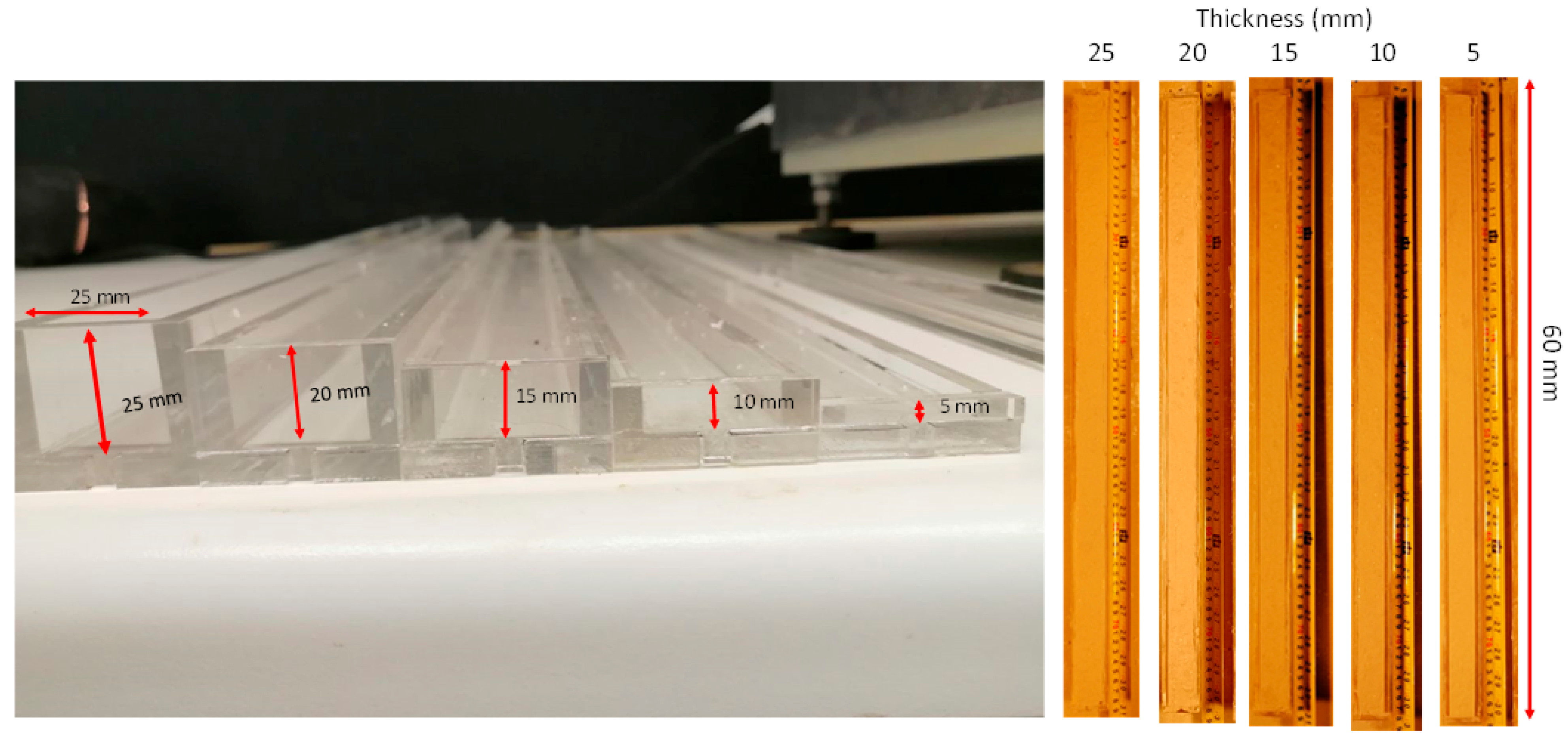
The cracking test plan included five different soil layer thicknesses, 5, 10, 15, 20 and 25 mm, based on previous laboratory tests on desiccation cracking [25]. For achieving the desired thickness, rectangular acrylic molds with widths and lengths of 25 and 600 mm, respectively, and target heights were prepared (Figure 1).

Soil mixtures were prepared at LL and 1.5 LL moisture contents and were cured for 24 h at room temperature to attain moisture equilibrium. During filling, air bubbles were removed from the sample by tapping for 30 s.

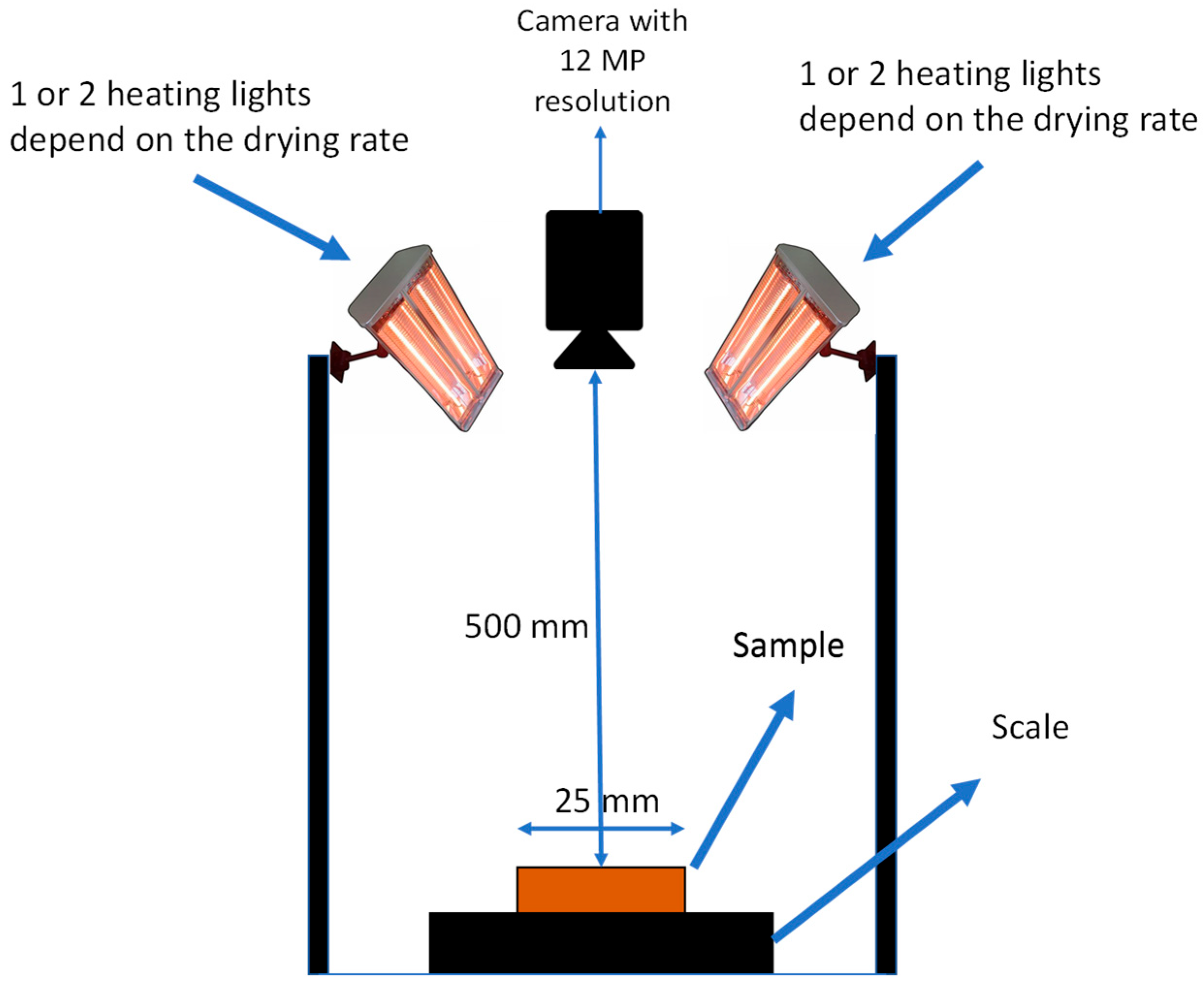
Two different drying rates were used, controlled by four lights over the length of the sample: for a higher drying rate (D), all four lights were on, and for a lower drying rate (0.75 D), two lights were on. Figure 2 shows the schematic drawing of the setup used for the drying tests.

All drying tests were conducted in a closed indoor laboratory environment to maintain consistency across experiments. While ambient temperature and relative humidity were allowed to vary slightly to reflect realistic conditions, their range was narrow—between 39.8 °C and 50.0 °C for temperature, and 15.9% to 17.9% for relative humidity—as listed in Table 2. No airflow or wind sources were present during the tests. These conditions ensured minimal environmental noise and a high consistency in the drying process, providing a reliable basis for model training and validation.

All tests were conducted for a duration of 270 min, and the drying rate was measured accordingly by using Equation (1) for each test. The drying rate ($D$) was assumed to be uniform during the drying period, as given by Equation (1).

$$D={\displaystyle \frac{m_f-m_i}{t}}$$

(1)

where $m_f$ is the final sample mass, $m_i$ is the initial sample mass and t is the total test time. The surrounding ambient temperature and humidity were also recorded during the drying process.

2.3. Shrinkage and Crack Quantification

In order to quantify shrinkage and cracks, images were taken every 30 min with a 12-megapixel camera. The final Crack and Shrinkage Intensity Factor (CSIF) was calculated using the final image taken after 270 min at the end of the test. The image analysis software ImageJ (Version 1.51) [26] was used to analyze the images and to calculate CSIF according to Equation (2).

CSIF = (Area of cracks and shrinkage)/(Initial sample area before drying)

(2)

2.4. Modeling Methods

2.4.1. Multiple Linear Regression (MLR)

Multiple Linear Regression (MLR) is a fundamental statistical technique used to model the relationship between a dependent variable and multiple independent variables through a linear equation. It estimates regression coefficients by minimizing the sum of the squared differences between observed and predicted values, allowing for the straightforward interpretation of each input’s contribution to the output. While MLR is computationally efficient and easy to implement, it inherently assumes linearity, independence and homoscedasticity among variables. These assumptions may limit its predictive performance when modeling highly non-linear processes such as soil desiccation cracking. Despite this, MLR serves as a useful baseline model for comparison with the more advanced machine learning techniques explored in this study.

2.4.2. Classification and Regression Random Forest (CRRF)

Breiman [27] combined decision trees with bootstrap aggregation or bagging to reduce classification and regression errors. Classification and Regression Random Forest (CRRF) is an ensemble learning method that combines multiple decision trees to improve predictive performance and reduce overfitting. Developed by Breiman [27], the random forest algorithm constructs numerous decision trees using bootstrap samples of the training data and random subsets of input variables at each split. For regression tasks, such as predicting the Crack and Shrinkage Intensity Factor (CSIF), the model aggregates the outputs of individual trees by averaging their predictions. This method is particularly robust when handling non-linear relationships, noisy data and complex interactions between variables. CRRF also provides insights into variable importance by evaluating the contribution of each input to the overall reduction in prediction error. Due to its simplicity, high accuracy and resistance to overfitting, CRRF is widely adopted in geotechnical engineering applications and serves as a reliable benchmark for evaluating model performance in this study.

2.4.3. Artificial Neural Network (ANN)

The ANN is a mathematical model composed of artificial neurons capable of finding complex, non-linear relationships between inputs and outputs. The ANN first identifies the relationship between inputs and outputs based on the weights that are the connecting power between two neurons [28]. Second, the network seeks to optimize the obtained weights, which is called the paradigm. This study used a feedforward paradigm [29], one of the strongest and most widely used paradigms. The feedforward paradigm has different algorithms. Bayesian Regularization (BR) [30] and Levenberg–Marquardt (LM) [31] algorithms with a strong ability in testing non-linear relationships were used in this study.

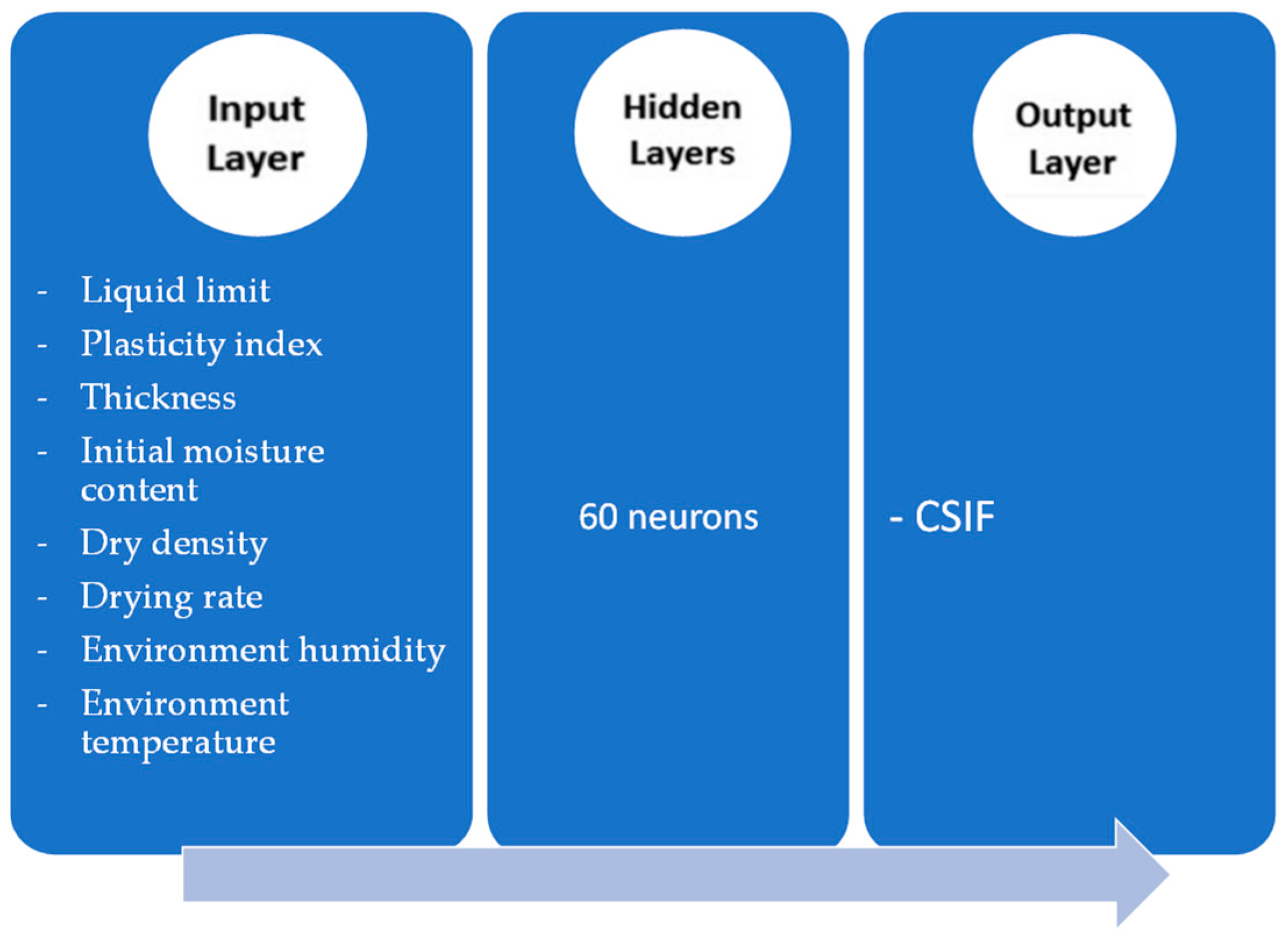
Input layers, hidden layers and output layers make up the ANN architecture. A total of five architecture types were considered, including one, two, three, four and five hidden layers, for each algorithm, LM and BR. The number of 60 neurons was selected after several trials. Each neuron was re-trained five times in every network. Figure 3 shows the ANN schematic architecture used in this study.

2.4.4. Genetic Programming (GP)

Genetic Programming (GP) is an evolutionary algorithm-based method that automatically evolves mathematical models or symbolic expressions to solve complex regression or classification problems. Inspired by the principles of natural selection and genetics, GP iteratively refines a population of candidate solutions—represented as computer programs or symbolic equations—through operations such as selection, crossover and mutation. In this study, GP was employed to derive explicit mathematical expressions for predicting the Crack and Shrinkage Intensity Factor (CSIF) using normalized input variables. Unlike traditional black-box models, GP offers interpretable and deployable formulas that can be directly used in practical engineering design without requiring specialized software. While GP may require significant computational effort and careful tuning to avoid overfitting, its ability to discover non-linear relationships and generate human-readable equations makes it a powerful tool for knowledge discovery and predictive modeling in geotechnical applications.

2.5. Data Processing

Drying tests resulted in 100 datasets with 8 effective inputs: dry density, initial water content, soil thickness, drying rate, LL, PI, ambient humidity and temperature; and one output parameter: the CSIF. The following steps were taken to prepare the database:

2.5.1. Normalization

In the existing database, each variable had its own unit. Data normalization reduces network error and increases the network training speed. Below is the normalization linear function which was used in this study.

$$X_{norm}={\displaystyle \frac{X-X_{min}}{X_{max}-X_{min}}}$$

(3)

where X_max, X_min, X and X_norm are the maximum, minimum, actual and normalized values, respectively.

2.5.2. Testing and Training Databases

For all three mathematical models, the dataset was randomly divided into two subsets: 80% for training and 20% for testing. To ensure the consistency and reliability of the model performance, the statistical characteristics of both subsets, along with the minimum, maximum, mean and standard deviation, were examined. As shown in

Table 3. Statistical information of training database.

Variable	Observations	Minimum	Maximum	Mean	Std. Deviation
CSIF	80	4.133	57.898	25.610	11.929
The drying rate (g/min)	80	0.142	0.252	0.207	0.031
Humidity (%RH)	80	15.900	17.900	16.850	1.005
Temperature (c)	80	39.800	50.000	44.645	5.126
Initial moisture (%)	80	71.097	312.500	175.452	71.677
LL	80	74.000	205.000	135.650	46.829
PI	80	40.000	169.000	100.709	46.114
Dry density	80	265.000	862.667	502.019	169.160
The thickness (mm)	80	5.000	25.000	14.625	7.016

and

Table 4. Statistical information of testing database.

Variable	Observations	Minimum	Maximum	Mean	Std. Deviation
CSIF	20	10.394	50.591	26.174	11.997
The drying rate (g/min)	20	0.148	0.250	0.213	0.034
Humidity (%RH)	20	15.900	17.900	17.100	1.005
Temperature (c)	20	39.800	50.000	45.920	5.127
Initial moisture (%)	20	74.439	249.300	158.787	48.480
LL	20	74.000	205.000	141.400	42.503
PI	20	40.000	169.000	106.371	41.854
Dry density	20	342.933	832.000	516.370	142.730
The thickness (mm)	20	5.000	25.000	16.500	7.452

, the training and testing datasets exhibited similar statistical distributions, indicating that the data segmentation was balanced and suitable for accurate model evaluation.

For a more comprehensive assessment, k-fold cross-validation (e.g., 5-fold or 10-fold) could be implemented, especially in future studies involving larger and more diverse datasets. This would allow each data point to be used for both training and validation, thereby minimizing variance and better capturing the model’s generalization capability. Although computational constraints limited its implementation in the current work—especially given the extensive hyperparameter tuning and re-training required for the ANN and GP models—we recognize its importance and recommend cross-validation as a key component in future extensions of this research.

3. Results

The experimental results obtained from the soil cracking tests and the results from the mathematical models are presented in the following sections.

3.1. Experimental Results from Cracking Tests

Based on the test plan in Table 2, 100 desiccation cracking tests were conducted under different test conditions. Figure 4 illustrates the CSIF data obtained from the cracking tests. The change in CSIF with dry density and layer thickness followed the patterns identified by previous researchers [22,23].

3.2. Effect of Input Variables

An important factor in network accuracy is the selection of input parameters. Five groups of MLR, CRRF and ANN models were evaluated for their impact on network accuracy (each ANN group contained ten ANNs, five networks with LM algorithms and five networks with BR algorithms).

Table 5. Different groups of ANN modeling with their input variables.

Group No.	Input Variables
	Dry Density	Thickness	Drying Rate	Initial Water Content	Liquid Limit (LL)	Plasticity Index (PI)	Ambient Temperature	Ambient Humidity
1	√	√	√	√	√	√	√	√
2	√	√	√	√	√	√	×	×
3	√	√	√	×	√	√	×	×
4	√	√	×	√	√	√	×	×
5	√	√	×	×	√	√	×	×

shows the five input groups that were run with mathematical models.

3.3. Mathematical Modeling Results

The correlation coefficient (R) and mean absolute error (MAE) between the predicted and measured values were used to assess the model’s performance. R and MAE are defined in Equations (4) and (5).

$$R={\displaystyle \frac{{\sum }_N(X_m-\overline{X_m})(X_p-\overline{X_p})}{\sqrt{{\sum }_N{(X_m-\overline{X_m})}^2}{\sum }_N{(X_p-\overline{X_p})}^2}}$$

(4)

$$MAE={\displaystyle \frac{{\sum }_N\left|\left(X_m-X_p\right)\right|}{N}}$$

(5)

where X_m, X_p, $\overline{X_m}$ and $\overline{X_p}$ are the actual value, predicted value, the average of actual value and the average of predicted value, respectively, and N is the number of datasets. The ideal model is the one that has an R of 1 and an MAE equal to 0.

3.3.1. Multiple Linear Regression (MLR)

The Pearson correlation matrix of parameters is shown in

Table 6. Correlation matrix of parameters.

	Drying Rate	Ambient Humidity	Ambient Temperature	Initial Moisture	LL	PI	Dry Density	Thickness	CSIF
Drying rate	1	0.904	0.904	0.214	0.195	0.195	−0.231	0.290	0.335
Humidity	0.904	1	1.000	0.046	0.025	0.025	−0.050	−0.021	0.408
Temperature	0.904	1.000	1	0.046	0.025	0.025	−0.050	−0.021	0.408
Initial moisture	0.214	0.046	0.046	1	0.870	0.870	−0.947	0.010	0.692
LL	0.195	0.025	0.025	0.870	1	1.000	−0.888	−0.007	0.750
PI	0.195	0.025	0.025	0.870	1.000	1	−0.888	−0.007	0.750
Dry density	−0.231	−0.050	−0.050	−0.947	−0.888	−0.888	1	−0.015	−0.689
Thickness	0.290	−0.021	−0.021	0.010	−0.007	−0.007	−0.015	1	−0.452
CSIF	0.335	0.408	0.408	0.692	0.750	0.750	−0.689	−0.452	1

. There is a strong correlation between ambient temperature and humidity and the drying rate, which is expected. The other inputs do not show any significant correlation, which indicates that multicollinearity does not affect them. More importantly, the correlation between inputs and the CSIF is less than 75%, which indicates that MLR cannot adequately predict CSIF. This affirms the non-linear nature of the desiccation cracking problem and the need for more sophisticated models to capture the cracking process accurately.

Figure 5 shows the actual and predicted values of CSIF for the training and testing databases for input groups 3 and 4. Based on the results of the MLR method, several points failed to meet 80% accuracy across all groups of databases.

Based on the R and MAE values shown in

Table 7. Results of MLR models for different databases and groups.

Group Number	Number of Inputs	Inputs	Training Database		Testing Database
			R	MAE	R	MAE
1	8	Dry density, thickness, drying rate, initial water content, liquid limit, plasticity index, ambient temperature, ambient humidity	0.853	10.412	0.847	10.447
2	6	Dry density, thickness, drying rate, initial water content, liquid limit, plasticity index	0.851	11.532	0.843	11.799
3	5	Dry density, thickness, drying rate, liquid limit, plasticity index	0.844	11.341	0.838	11.499
4	5	Dry density, thickness, initial water content, liquid limit, plasticity index	0.759	12.274	0.750	12.045
5	4	Dry density, thickness, liquid limit, plasticity index	0.734	15.376	0.721	15.674

, input group 1 achieves the best MLR performance. Groups 1, 2 and 3 show small differences in R, while groups 4 and 5 show much lower R. The selection of input parameters in group 3 can be considered the optimum combination according to Table 7.

3.3.2. Classification and Regression Random Forest (CRRF)

Table 8. The specifications of the best CRRF.

Tree Parameters					Forest Parameters
Min. Node Size	Min. Son Size	Max Depth	Mtry	CP	Sampling	Sample Size	Number of Trees
2	1	10	2	0.00001	Random with replacement	100	1000

lists the tree and forest parameters used in the CRRF model. M_try is the number of random subsets of variables per node. Increasing the number of trees increased the analysis time. In addition, the accuracy of the tree increased with depth until it reached 10, then declined, so 10 was the optimal depth.

Figure 6 shows the actual and predicted values for CSIF for input groups 3 and 4, both for the training and test databases. Group 3 slightly outperforms group 4 in terms of the R and MAE values. The results for all five input groups are shown in

Table 9. The performance of the best CRRF model at predicting CSIF.

Group Number	Number of Inputs	Inputs	Training Database		Testing Database
			R	MAE	R	MAE
1	8	Dry density, thickness, drying rate, initial water content, liquid limit, plasticity index, ambient temperature, ambient humidity	0.983	5.926	0.974	6.008
2	6	Dry density, thickness, drying rate, initial water content, liquid limit, plasticity index	0.978	6.062	0.965	6.329
3	5	Dry density, thickness, drying rate, liquid limit, plasticity index	0.981	6.492	0.967	6.978
4	5	Dry density, thickness, initial water content, liquid limit, plasticity index	0.867	7.914	0.853	8.066
5	4	Dry density, thickness, liquid limit, plasticity index	0.810	9.075	0.789	9.966

. In the first three databases, namely groups 1, 2 and 3, the models have high R, while in the fourth and fifth databases, the models have lower R. However, group 3 can be considered the most desired database since it has fewer input parameters. The R value for group 3 is 0.97, which indicates good accuracy and performance.

3.3.3. Artificial Neural Network (ANN)

Table 10. The ANN results for group 1 with eight inputs.

Model	R		MAE
	Testing Database	Training Database	Testing Database	Training Database
BR-1H	0.992	0.999	5.377	4.418
BR-2H	0.989	0.999	5.630	4.195
BR-3H	0.981	0.999	5.988	4.197
BR-4H	0.935	0.928	10.231	10.063
BR-5H	0.928	0.916	11.673	10.703
LM-1H	0.989	0.997	5.664	4.528
LM-2H	0.991	0.998	5.375	4.575
LM-3H	0.990	0.997	5.525	4.527
LM-4H	0.991	0.997	5.328	4.499
LM-5H	0.994	0.998	5.449	4.473

,

Table 11. The ANN results for input group 2 with six inputs.

Model	R		MAE
	Testing Database	Training Database	Testing Database	Training Database
BR-1H	0.991	0.999	5.246	4.425
BR-2H	0.990	0.999	5.411	4.436
BR-3H	0.983	0.999	5.858	4.185
BR-4H	0.983	0.999	5.801	4.399
BR-5H	0.896	0.885	11.745	12.082
LM-1H	0.989	0.996	5.643	4.693
LM-2H	0.987	0.996	5.758	4.495
LM-3H	0.990	0.997	5.883	4.506
LM-4H	0.983	0.999	5.801	4.399
LM-5H	0.991	0.997	5.464	4.530

,

Table 12. The ANN results for input group 3 with five inputs.

	R-Test	R-Train	MAE-Test	MAE-Train
BR-1H	0.990	0.999	5.471	4.327
BR-2H	0.991	0.999	5.443	4.537
BR-3H	0.988	0.999	5.825	4.149
BR-4H	0.979	0.999	6.403	4.158
BR-5H	0.944	0.915	9.714	10.082
LM-1H	0.987	0.997	5.575	4.660
LM-2H	0.988	0.996	5.773	4.609
LM-3H	0.986	0.998	5.724	4.526
LM-4H	0.987	0.997	5.759	4.518
LM-5H	0.989	0.997	5.554	4.490

,

Table 13. The ANN results for group 4 with five inputs (excluding drying rate).

	R-Test	R-Train	MAE-Test	MAE-Train
BR-1H	0.904	0.904	8.092	8.388
BR-2H	0.904	0.904	8.092	8.357
BR-3H	0.898	0.904	9.146	8.377
BR-4H	0.896	0.908	9.209	8.307
BR-5H	0.898	0.876	10.464	10.405
LM-1H	0.910	0.928	7.922	7.562
LM-2H	0.910	0.933	8.017	7.800
LM-3H	0.899	0.920	8.330	7.676
LM-4H	0.933	0.924	8.329	7.502
LM-5H	0.920	0.926	8.196	7.693

and

Table 14. The ANN results for input group 5 with four inputs.

Model	R		MAE
	Testing Database	Training Database	Testing Database	Training Database
BR-1H	0.905	0.912	8.012	8.245
BR-2H	0.905	0.910	8.004	8.231
BR-3H	0.875	0.905	9.162	8.362
BR-4H	0.898	0.905	9.189	8.360
BR-5H	0.901	0.907	9.435	8.324
LM-1H	0.920	0.920	8.057	7.552
LM-2H	0.911	0.916	7.758	7.797
LM-3H	0.911	0.920	8.122	7.408
LM-4H	0.905	0.921	8.196	7.667
LM-5H	0.913	0.922	8.370	7.699

present the ANN results for each input group for different algorithms and hidden layers. The ANN with five hidden layers using the LM algorithm was the best model for group 1. For the testing database, this model resulted in an R of 0.994 and MAE of 5.449. Hence, this network was sufficiently accurate.

The LM algorithm network with five hidden layers had the best accuracy with R and MAE values of 0.991 and 5.464, respectively, for the second input group as well (see Table 11). Despite removing ambient temperature and humidity, the network accuracy was still high, and as shown by the MLR analysis in Section 3.3.1, the effect of ambient temperature and humidity can be accounted for by the drying rate.

The R and MAE values of the ANN for input group 3 are shown in Table 12. Using the BR algorithm (with two hidden layers), the best ANN model had an R of 0.991 and MAE of 5.443. In this model, the network accuracy remained high even after removing initial moisture content, ambient temperature and humidity. The low significance of initial moisture content was due to initial moisture content being prepared as a function of the liquid limit (LL and 1.5 LL), which reduced the importance of initial water content as an independent influential factor.

The results for input group 4 of the training and testing databases are shown in Table 13. Compared to group 3, the R value of the highest performing algorithm dropped to 0.93. This sharp drop in model accuracy suggests the importance of drying rate in crack prediction. The model with four hidden networks and the LM algorithm was the best for group 4.

The best ANN model for input group 5 had an R of 0.92 and MAE of 8.05, as shown in Table 14. This model was based on the LM algorithm with one hidden layer. Although the network’s accuracy decreased slightly from 0.93 to 0.92, it was approximately the same as group 4. Thus, it was affirmed that the removal of initial soil water content did not significantly affect the accuracy of the predictions.

Comparing Table 10, Table 11, Table 12, Table 13 and Table 14, it can be concluded that input group 3 is the most appropriate combination of input parameters for desiccation crack prediction. Group 3 achieved almost the same accuracy as groups 1 and 2, but with fewer inputs. Hence, it was the most optimal of the five input groups. The CSIF results predicted by the best network for group 3 are shown in Figure 7. There is excellent agreement between the actual and predicted CSIF values.

The number of hidden layers (ranging from 1 to 5) and neurons per layer (fixed at 60) were selected based on extensive trial-and-error optimization. Each network configuration was evaluated five times, and the average R and MAE values were compared to identify the best-performing structure. The choice of 60 neurons per layer was found to offer a strong balance between training stability and model complexity, while deeper networks (e.g., 4 or 5 layers) tended to slightly overfit the data without significant gains in prediction accuracy.

3.3.4. Genetic Programming (GP)

The Genetic Programming method represents a technique capable of generating novel equations. This approach involves the introduction of diverse functions into the model, allowing the formulation of the desired equation based on these functions. In desiccation cracking, among the essential parameters considered, the drying rate stands out [32]. Previous studies have demonstrated that crack evolution, modeled by an exponential function, is a function of the drying rate. For example, El Youssoufi et al. [33] proposed a pragmatic model for soil drying kinetics that took into account the changes in the grain radius R over time during the drying process.

$$R=R_0 \mathrm{e}\mathrm{x}\mathrm{p}(-\alpha {\displaystyle \frac{t}{\tau }})$$

(6)

where R₀ is the radius at t = 0, α is a shrinkage parameter and τ is the total duration of the experiment.

The proposed GP model assumes the use of the exponential function in Equation (6). Notably, Equation (7), which comprises five inputs, is presented for the first time and the values in the equation are normalized based on Table 4. To use this equation, normalization must be performed linearly using the values provided in Table 4.

CSIF = (R₁× (((((R₂ − X₅) × (2 × X₅)) × ((X₂ − X₁) + (exp(R₁)))) × (((X₅ − R₁) × (R₂ + X₃)) + ((X₄ × R₁) − (R₁ + R₂)))) − ((X₅ – ((X₅²) + (X₃ − X₅))) − ((R₂ − (X₁ × X₄)) + ((exp(X₁)) − (X₅ − X₂))))))

(7)

where X₁, X₂, X₃, X₄ and X₅ are drying rate, LL, PI, dry density and thickness. R₁ and R₂ are 0.170 and 0.963.

Equation (8) represents the second equation proposed to estimate CSIF. In this equation, the ${\mathrm{x}}^{{\displaystyle \frac{1}{3}}}$ function is utilized.

$$\mathrm{CSIF}=({\mathrm{R}}_1\times ((({{\mathrm{R}}_1}^{{\displaystyle \frac{1}{3}}}-\left(\right({\mathrm{X}}_4\times \mathrm{R}1)\times ({{\mathrm{X}}_1}^2\left)\right))-(({\mathrm{X}}_4\times ({\mathrm{X}}_5-{\mathrm{X}}_4\left)\right)\times \left(\right({\mathrm{X}}_1-{\mathrm{X}}_2)\times ({\mathrm{X}}_5-{\mathrm{R}}_2\left)\right)\left)\right)+({\mathrm{X}}_1+({\mathrm{X}}_3-{{\mathrm{X}}_5}^{{\displaystyle \frac{1}{3}}}))))$$

(8)

where X₁, X₂, X₃, X₄ and X₅ are drying rate, LL, PI, dry density and thickness. R₁ and R₂ are 0.374 and 0.460.

Table 15. The performance of two proposed GP equations for group 3 with five inputs.

Proposed Model	R		MAE
	Testing Database	Training Database	Testing Database	Training Database
Equation (7)	0.947	0.970	2.527	2.039
Equation (8)	0.958	0.973	2.431	2.048

reports the accuracy of both equations, and the results demonstrate that Equation (7) achieves a higher accuracy than Equation (8). These findings suggest that cracking modeled by a function of ${\mathrm{x}}^{{\displaystyle \frac{1}{3}}}$ represents a function of the drying rate.

Comparing Equations (7) and (8), it can be seen that Equation (8) outperforms Equation (7) in both the R-Test and MAE-Test metrics. This indicates that Equation (8) has better predictive power on both the training and testing databases, and it makes fewer errors in predicting the target variable.

Figure 8 illustrates the anticipated CSIF values by the proposed Equations (7) and (8) against the actual values obtained during the experiments for training and testing. The outcomes presented in Figure 8 indicate that both proposed equations were able to predict the values of CSIF accurately. The close alignment between the model’s anticipated values and the actual values obtained indicates the model’s high accuracy in forecasting CSIF values.

4. Discussion

4.1. Comparison of Mathematical Models

The results of the four mathematical models used to predict CSIF using the five input groups are presented in

Table 16. Comparison of model performances (MLR, CRRF, ANN and GP) at predicting CSIF across different input groups.

Group Number	Number of Inputs	Mathematical Methods						Proposed GP Equation
		MLR		CRRF		ANN
		R	MAE	R	MAE	R	MAE	R	MAE
1	8	0.847	10.447	0.97	6.01	0.99	5.45
2	6	0.843	11.799	0.96	6.33	0.99	5.46
3	5	0.838	11.499	0.97	6.98	0.99	5.44	0.958	2.431
4	5	0.750	12.045	0.85	8.07	0.93	8.33
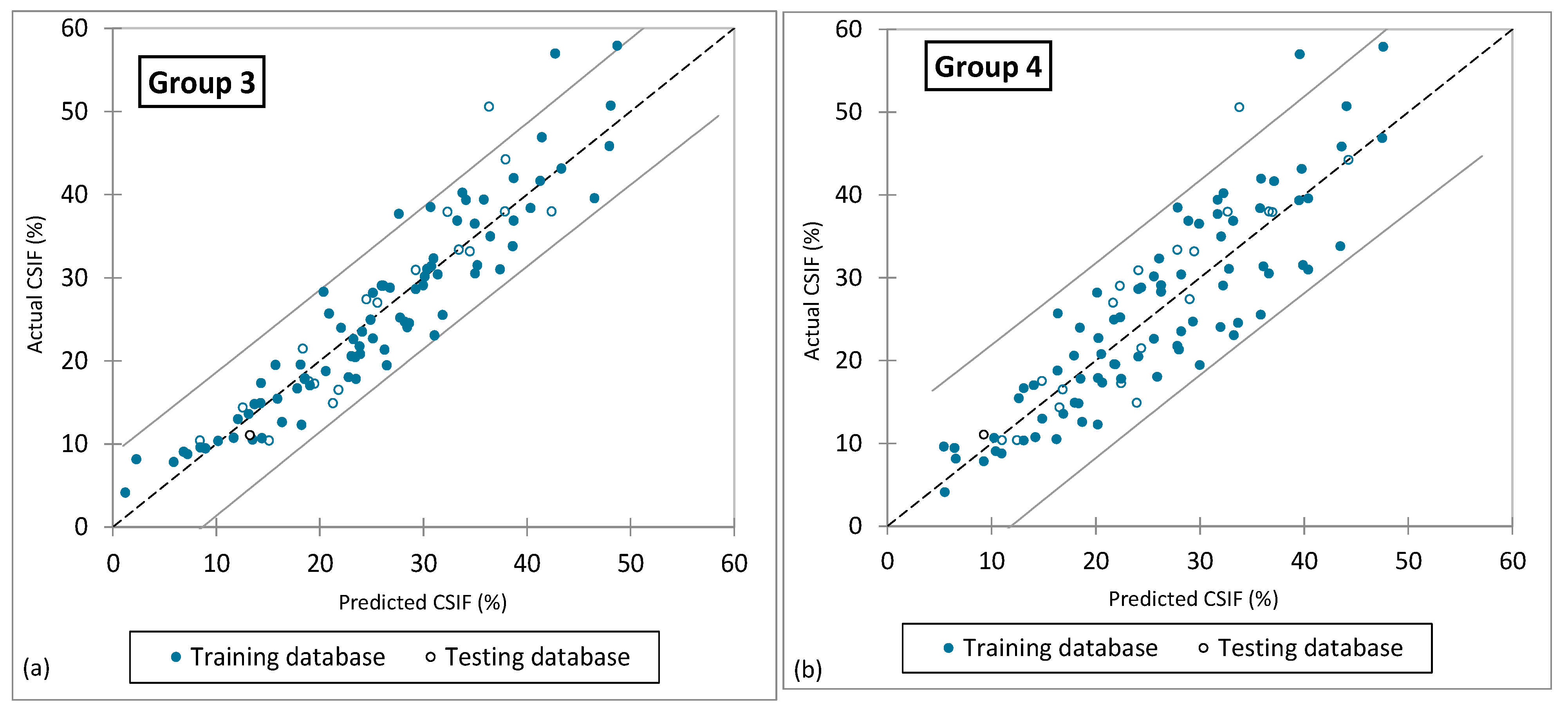
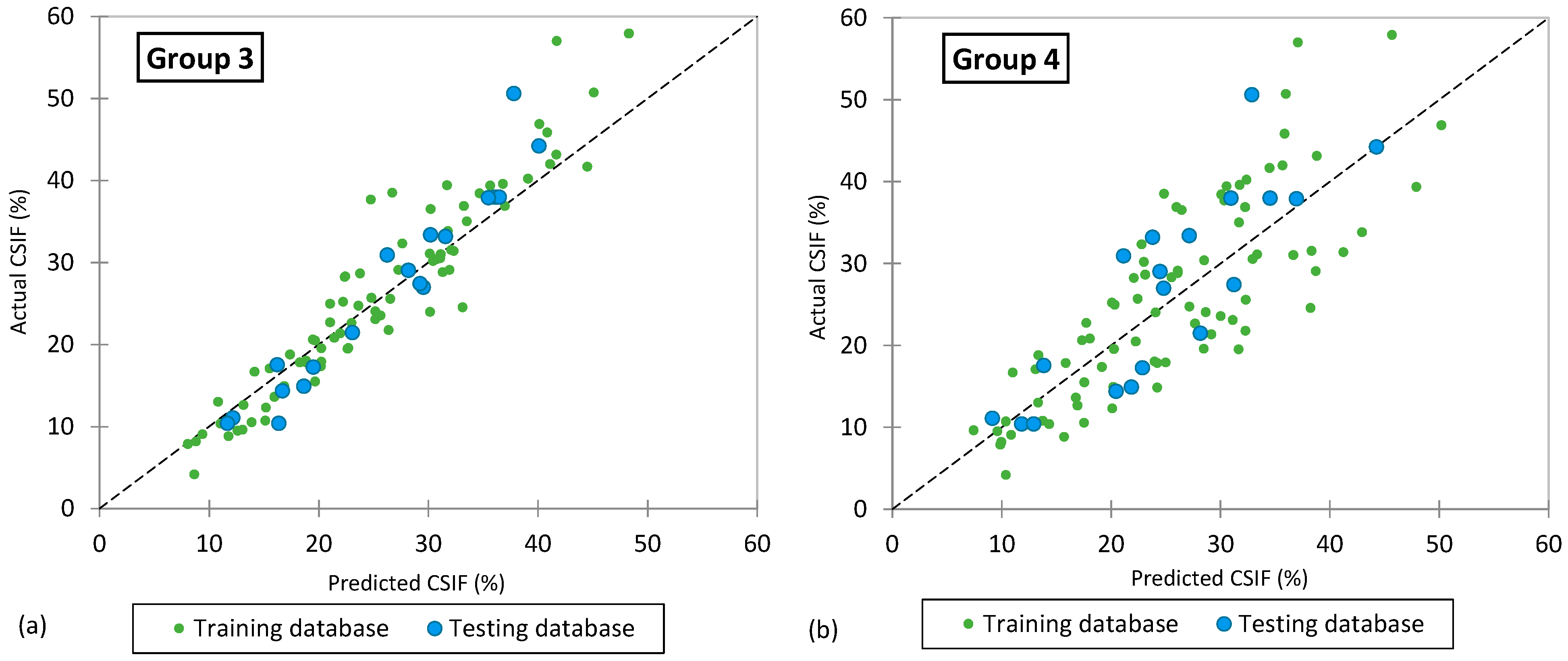
5	4	0.721	15.674	0.79	9.97	0.92	8.05

. Based on the R values of the three mathematical models using the first three input groups, 1, 2 and 3, the initial moisture content, ambient temperature and humidity did not appear to have much impact on prediction when drying rate was included. When drying rate was removed, the accuracy of all three mathematical models was greatly reduced, indicating the importance of drying rate in predicting CSIF.

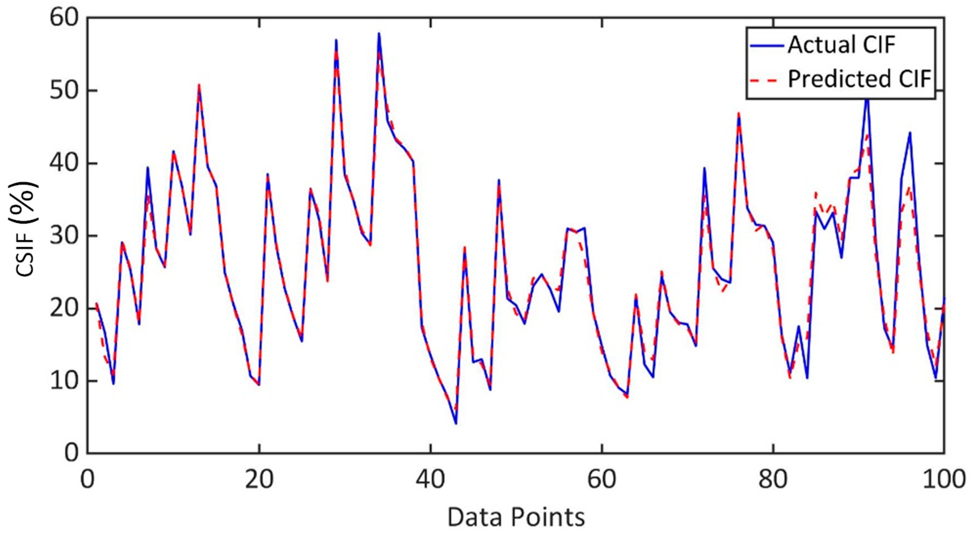
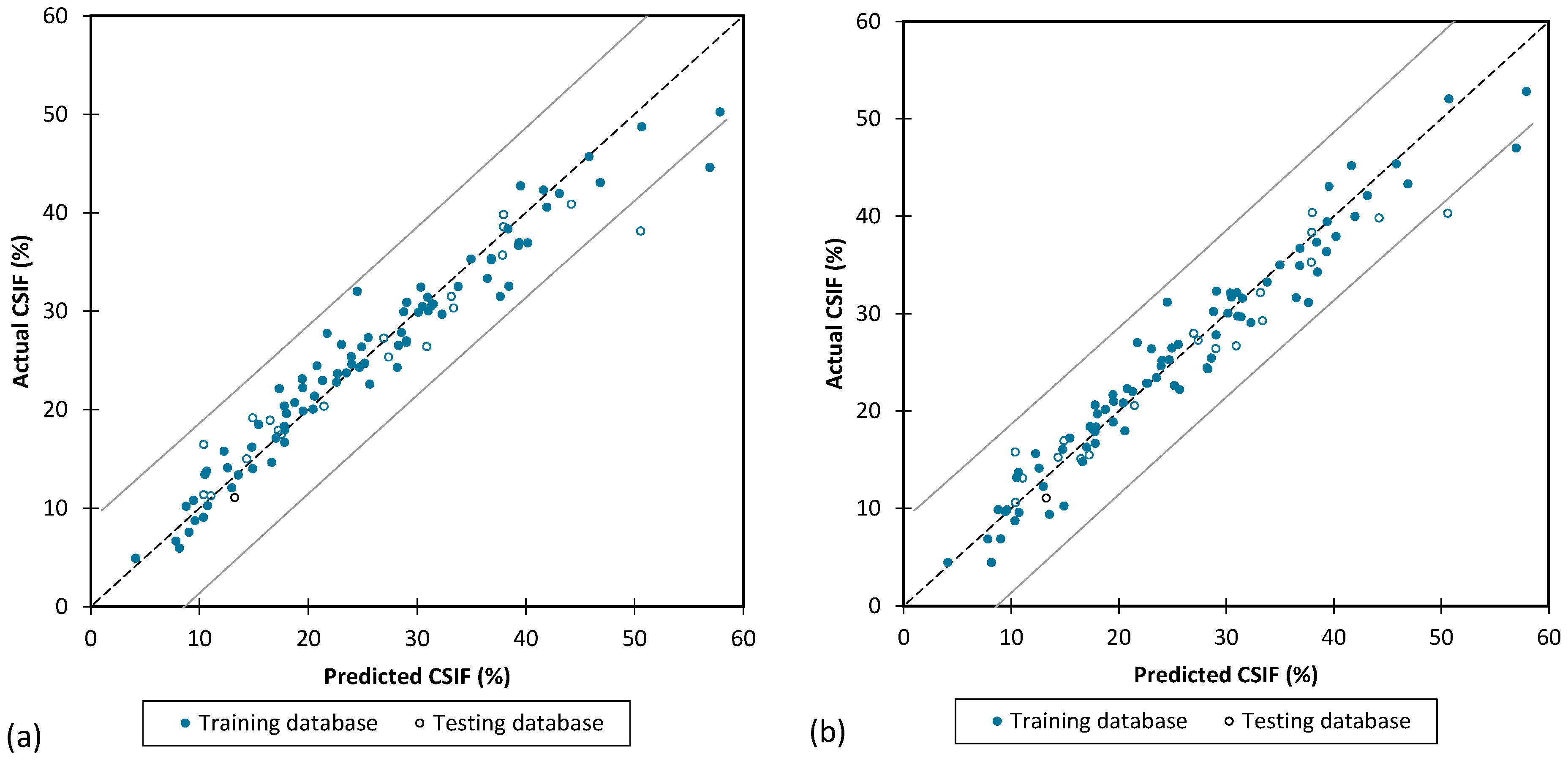
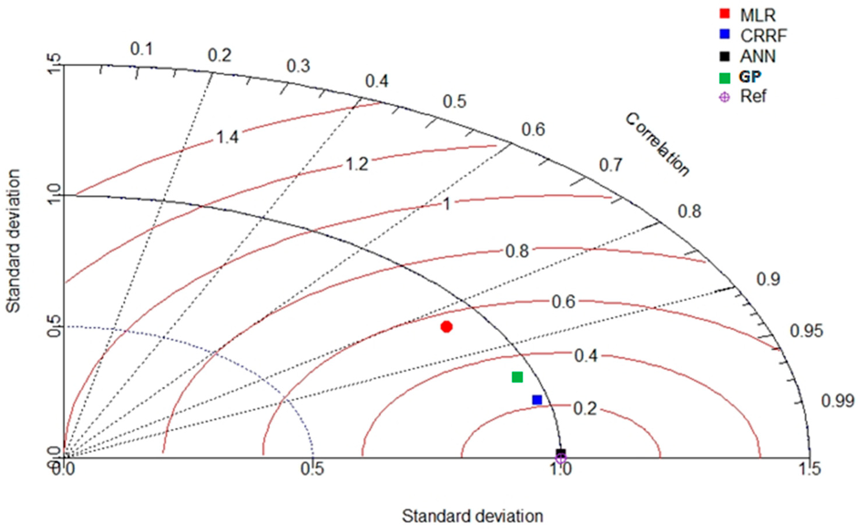
Among all five input groups, the Artificial Neural Network (ANN) consistently outperformed the other models, achieving the highest predictive accuracy with an R value of 0.99 and a mean absolute error (MAE) of approximately 5. The Classification and Regression Random Forest (CRRF) model ranked second in performance, particularly for input groups 1, 2 and 3, where it attained an R of 0.97 and an MAE close to 6. In contrast, the Multiple Linear Regression (MLR) model showed the lowest accuracy, with an R value around 0.84 and MAE value near 11 for the same input groups, highlighting its limitation in capturing the non-linear nature of this problem. Notably, the Genetic Programming (GP) model developed for input group 3 yielded an R of 0.958 and an exceptionally low MAE of 2.431, demonstrating strong predictive capability and enhanced interpretability.

Figure 9 presents the Taylor diagram for input group 3, identified as being the most optimal input combination. This diagram was used to compare the predictive performance of the mathematical models against the actual laboratory results for the testing dataset (denoted as REF in the figure). Among all models, the ANN demonstrated the closest agreement with the experimental data, confirming its superior accuracy and reliability in predicting the Crack and Shrinkage Intensity Factor (CSIF).

The ANN model outperformed the other approaches across all input groups, particularly when trained using Bayesian Regularization. Unlike traditional algorithms that focus solely on minimizing error, BR introduces a Bayesian inference framework to optimize network weights while constraining overfitting. This allows the network to remain flexible enough to model complex, non-linear interactions (e.g., between LL, PI and drying rate) while avoiding noise fitting, which was a limitation in both the MLR and over-parameterized networks. These characteristics make BR especially effective for geotechnical problems involving coupled processes with limited datasets.

4.2. Sensitivity Analysis of Input Parameters in ANN Models

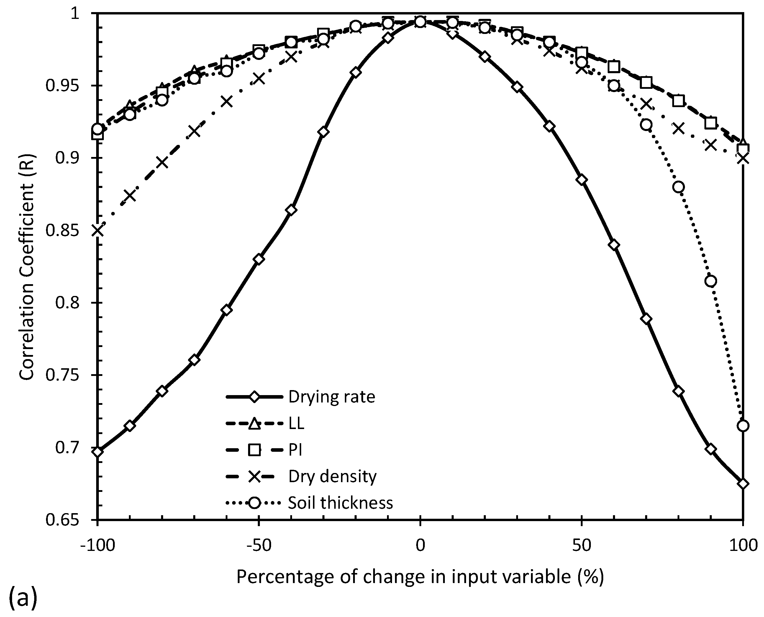
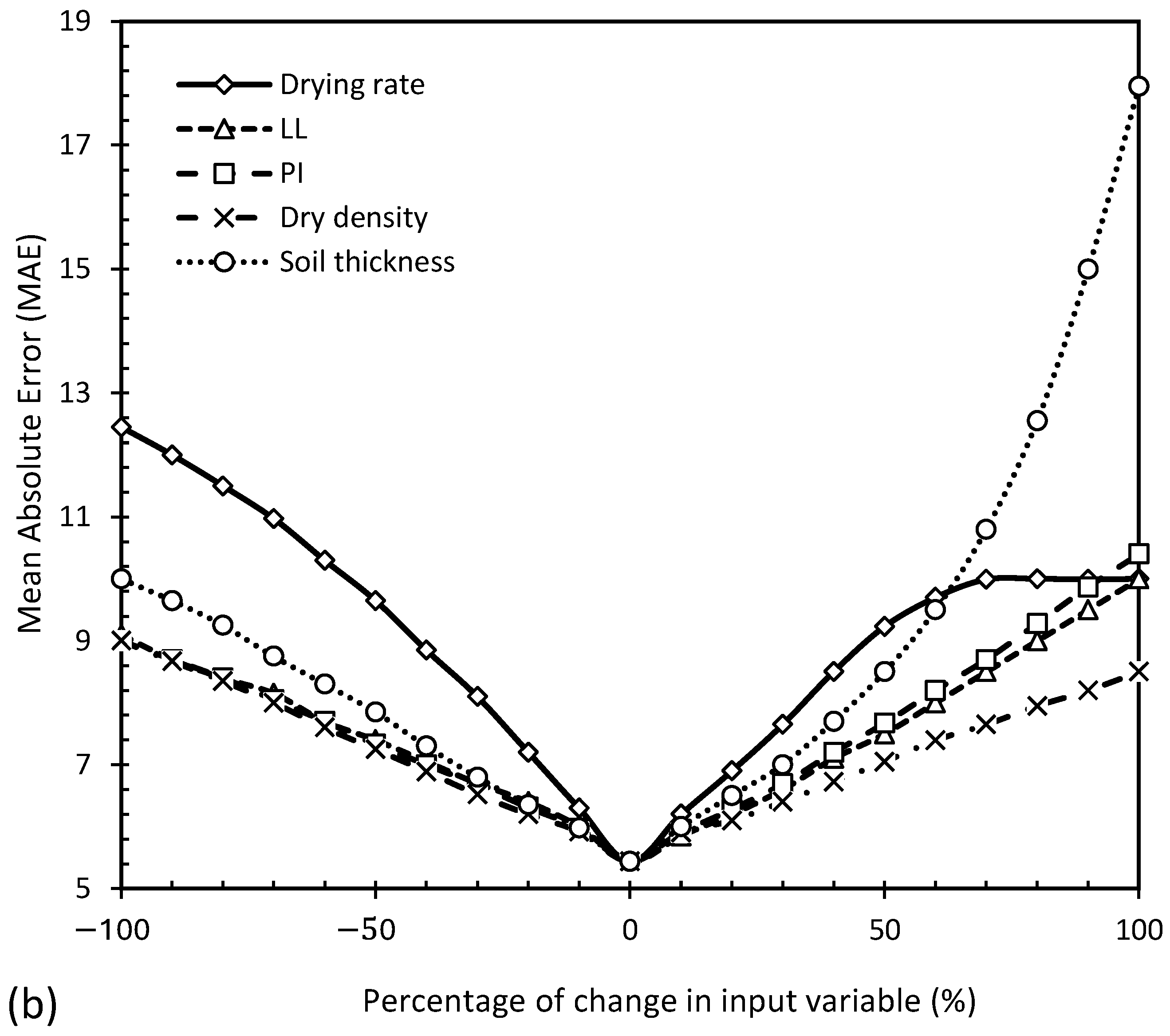
To assess the sensitivity, each input parameter was changed from −100% to +100% separately. The ANN model sensitivity analysis for the input parameters is shown in Figure 10.

Increasing or decreasing the drying rate by 100% decreased the R of the model to about 0.675 and increased the MAE to about 12.5. For LL, MAE was almost symmetrical with LL changes. In the worst-case scenario, when LL increased by 100%, R was reduced to about 0.9 and MAE was increased to about 10. For PI, the MAE of the ANN increased most when PI increased by 100%, resulting in a change in MAE to 10.4. In response to changing the dry density by 100%, the model’s R and MAE reached 0.85 and 9. Finally, for soil thickness, a 100% increase in soil thickness caused the largest network error (MAE). As soil thickness increased, R decreased to 0.715 and MAE increased to 17.95.

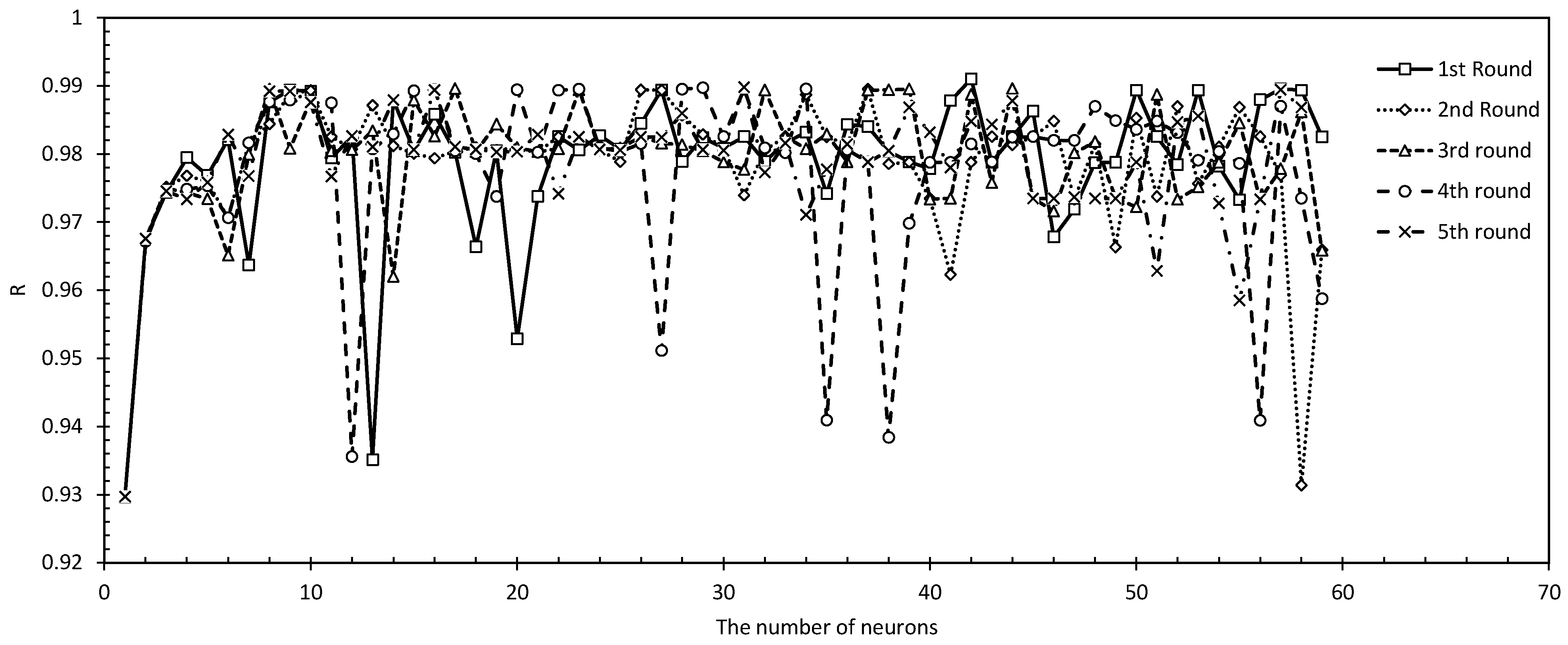
4.3. The Number of Neurons and Re-Training in the Best ANN Model

When modeling ANNs, layers, neurons and neuron re-training are important. Figure 11 illustrates the best ANN model with two hidden layers, using the BR algorithm, for various hidden neurons and network training numbers. Consequently, the ANN model had the greatest error (MAE) in the first and third network re-trainings, but the lowest error (MAE) in the second and fifth.

4.4. The Importance of the Input Parameters

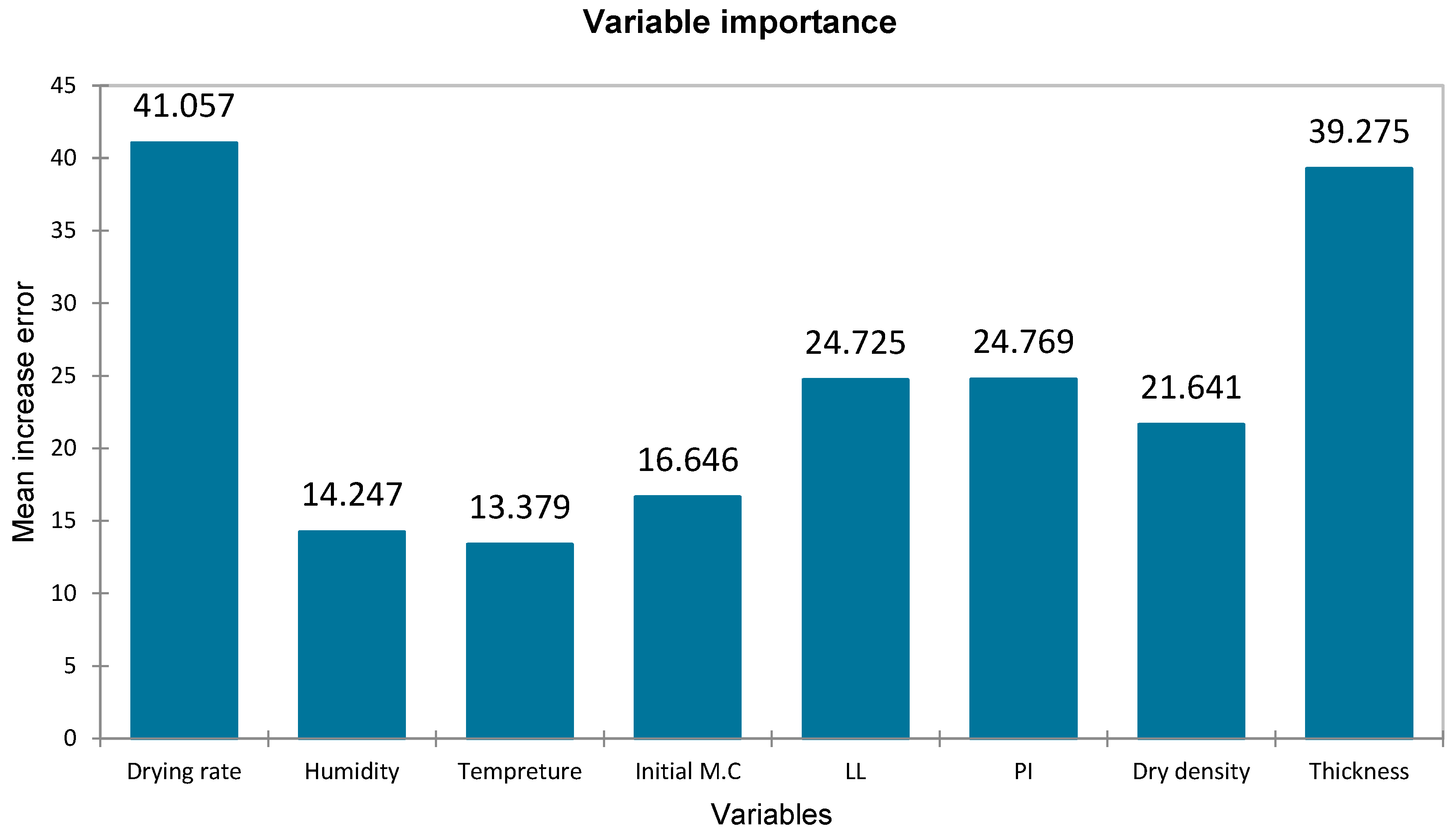
The CRRF and ANN models with two hidden layers using the BR algorithm were investigated for the influence of input parameters on MAE. Figure 12 shows the sensitivity of the best CRRF model to input parameters. The highest sensitivity was related to soil thickness and drying rate, while the lowest sensitivity was related to ambient humidity and temperature. Jamhiri et al. [19] also ranked temperature and relative humidity among the least influential parameters for desiccation cracking.

Table 17. The results of the importance of variables for three AI models.

	Input Parameters
	Drying Rate			Humidity			Temperature			Initial MC			LL			PI			Dry Density			Thickness
	ANN	CRRF	GP	ANN	CRRF	GP	ANN	CRRF	GP	ANN	CRRF	GP	ANN	CRRF	GP	ANN	CRRF	GP	ANN	CRRF	GP	ANN	CRRF	GP
MAE	2	1	1	7	7	8	8	8	7	6	6	6	4	4	5	3	3	4	5	5	3	1	2	2

presents the ranking of the importance of input parameters based on the increase in mean absolute error (MAE) observed in three AI models: ANN, CRRF and GP. Across all models, drying rate and soil thickness consistently emerged as the most critical factors influencing the prediction of the Crack and Shrinkage Intensity Factor (CSIF), with the lowest MAE rankings (1 or 2). In contrast, ambient humidity and temperature showed the lowest influence, receiving the highest MAE rankings (7 or 8), confirming their redundancy when drying rate was included. Intermediate significance was observed for the liquid limit (LL), plasticity index (PI), dry density and initial moisture content, with moderate MAE impacts across the models. These results aligned with the sensitivity analysis findings and emphasized the dominant role of drying dynamics and soil geometry in desiccation crack development.

Regarding the importance of drying rate, the results of Zhang et al. [34] showed that the drying rate had a significant effect on the total pore volume. They found that samples dried at higher drying rates had larger total pore volumes than those at lower drying rates. In addition, the experimental results of Krisdani et al. [35] confirmed that the changes in the proportion of empty space and the degree of soil saturation were strongly influenced by the rate of drying.

LL and PI were the third and fourth most significant and influential factors in predicting CSIF in three AI models, according to Table 17. LL and PI play an important role in affecting pore water volume and contraction strain. PI increases the pore water volume and therefore the volumetric shrinkage strain during drying, according to Rayhani et al. [36].

Dry density was the fifth most important parameter in both the ANN and CRRF and the third parameter in GP, followed by the initial moisture content, ambient humidity and temperature. Section 3.3.1, Section 3.3.2. and Section 3.3.3 discuss how the removal of these three parameters affects model accuracy.

The dominance of soil thickness and drying rate as the most important variables is consistent across all AI models tested. Thicker soil layers are more susceptible to crack propagation due to the greater energy required to overcome tensile strength and form multiple fracture planes. In contrast, thinner layers are more constrained and develop fewer cracks. The drying rate governs the rate of moisture loss, which directly influences suction generation, shrinkage strain accumulation and the initiation of desiccation cracking. Higher drying rates often result in steeper moisture gradients, leading to rapid crack formation and wider fracture networks. These behaviors are supported by the experimental findings from Costa et al. [37], Krisdani et al. [35] and Zhang et al. [34], all of whom observed significant changes in crack morphology with variations in thickness and drying conditions.

The effect of removing potentially redundant parameters, such as initial moisture content, was investigated through a comparison of different input groups. Notably, input group 3, which excluded initial moisture content, ambient temperature and humidity, achieved a nearly identical performance to groups 1 and 2, with an R of 0.991 and MAE of 5.44 for the testing dataset. This indicated that the removal of initial moisture content did not significantly affect the model’s predictive capability. This can be attributed to the experimental setup, in which initial moisture was fixed at either LL or 1.5 LL for each test case. As a result, the variation in initial moisture content was already embedded in the LL parameter, making its explicit inclusion redundant. This finding supports the idea that carefully reducing the number of input parameters can streamline the model, improve computational efficiency and reduce overfitting risks without compromising accuracy.

The sensitivity analysis results provide a clear understanding of how each input parameter affects prediction error and thus offers valuable insight for simplifying models without compromising accuracy. The dominant influence of drying rate and soil thickness aligns with physical observations from past studies, highlighting their role in controlling moisture migration and crack energy release. Such insights are useful for prioritizing field measurements when data availability is limited.

4.5. Sustainability and Future Research Directions

The application of AI-based models in predicting soil desiccation cracking contributes to sustainability in geotechnical engineering by minimizing the need for extensive physical testing and enabling the more efficient use of resources. The accurate prediction of crack intensity factors can assist engineers in proactively designing infrastructure and soil covers, thereby reducing long-term maintenance costs and the environmental impacts associated with soil failure and water seepage.

Furthermore, the reduced reliance on trial-and-error approaches for crack control in clayey soils promotes a more sustainable design methodology, especially in expansive soil regions where desiccation-related damage is common.

Future research should explore the generalization of these models to more complex crack geometries (2D and 3D patterns), as well as their validation in field-scale conditions under natural environmental variability. Incorporating additional environmental factors (e.g., wind speed, solar radiation), developing hybrid physical–AI models and creating lightweight predictive tools for field use (e.g., mobile apps or edge computing devices) are promising directions to enhance both the sustainability and practicality of this approach in real-world applications.

4.6. Comparison with Previous Studies

An ANN model was used by Choudhury and Costa [20] to predict 1D cracks in thin, long layers.

Table 18. The results of the proposed models using the training and testing databases by Choudhury and Costa [20] and the ANN (in this study).

Database	Proposed Models
	Choudhury and Costa [20]		ANN
	R	MAE	R	MAE
Training	0.92	7.55	0.99	4.53
Testing	0.93	7.25	0.99	5.44

compares the accuracy of predictions from this study to Choudhury and Costa [20]. The best performing model from each study has been selected for comparison. The current study achieved improved R and MAE values compared to Choudhury and Costa [20].

Earlier studies in the domain of desiccation crack prediction primarily focused on limited datasets and fewer input parameters. For instance, Choudhury and Costa [20] applied an ANN model to predict the number of cracks in long, thin clay layers based on only four input variables and a relatively small dataset of 16 samples. While they achieved high predictive accuracy (R = 0.93), their output was limited to the number of cracks, which did not fully reflect the severity or morphology of desiccation cracking.

In contrast, the current study introduces the Crack and Shrinkage Intensity Factor (CSIF) as a more comprehensive and continuous output variable that better captures the extent of desiccation damage. By developing a larger experimental database (n = 100) with eight physical and environmental input parameters, and by testing multiple AI and regression models, we present a more robust framework for crack prediction.

The ANN model in this study achieves R = 0.99 and MAE = 5.44, which represents a notable improvement over previous studies—not just numerically, but in terms of the model generalizability, input diversity and output quality. Furthermore, unlike past research, this study performs a detailed input sensitivity analysis and explores parameter optimization, including the effect of removing redundant inputs.

Additionally, the introduction of a symbolic Genetic Programming (GP) model adds interpretability and usability by providing analytical equations that can be easily deployed in engineering calculations. The inclusion of residual plots and Taylor diagrams further strengthens the reliability of the findings, going beyond simple correlation metrics.

5. Conclusions

A series of drying tests were conducted on five types of clay (with different LLs and PIs) in different conditions, including initial moisture content, ambient temperature and humidity, dry density, drying rate and soil thickness. This experimental database was used to predict the Crack and Shrinkage Intensity Factor (CSIF) using four mathematical models, namely MLR, CRRF, ANN and GP.

• The ANN models produced the most accurate predictions for CSIF, with an R of 0.99 and MAE of 5.44 for the testing database. Predictions from CRRF and GP were also satisfactory. A higher MAE was noticed in the MLR predictions, indicating the limitations of linear models in encapsulating non-linear processes in desiccation crack formation.
• Critical input parameters for AI modeling of desiccation cracks were identified: liquid limit, plasticity index, dry density, soil layer thickness and drying rate. Ambient temperature and humidity were deemed redundant when drying rate was included. Similarly, initial moisture content could also be omitted when liquid limit was included.
• The most sensitive input parameters to predict CSIF were soil layer thickness and drying rate followed by plasticity index, liquid limit and dry density.

From a practical engineering standpoint, the developed models can be used to support predictive assessments of soil cover performance, crack mitigation in clay liners and risk evaluations for expansive soil foundations. For example, the ANN model could be integrated into early-stage design tools to estimate the risk of shrinkage cracking under varying environmental conditions, enabling the more efficient selection of soil types or thicknesses. The symbolic GP equations further offer opportunities for fast estimations in field or design office settings without the need for complex software.

While the models developed in this study demonstrated excellent predictive performance under controlled laboratory conditions, further work is needed to assess their generalizability to real-world scenarios. Future research will aim to incorporate field data, explore climate variability and extend the models to 2D and 3D crack patterns. Additionally, integrating uncertainty quantification and cross-site validation will be essential for establishing the models as reliable tools in practical geotechnical applications.

References

1. Amarasiri, A.; Kodikara, J.; Costa, S. Numerical Modelling of Desiccation Cracking. Int. J. Numer. Anal. Methods Geomech. 2011, 35, 82–96. [Google Scholar] [CrossRef]
2. Amarasiri, A.; Kodikara, J. Use of material interfaces in DEM to simulate soil fracture propagation in mode I cracking. Int. J. Geomech. 2011, 11, 314–322. [Google Scholar] [CrossRef]
3. Gui, Y.L.; Zhao, Z.Y.; Kodikara, J.; Bui, H.H.; Yang, S.Q. Numerical modelling of laboratory soil desiccation cracking using UDEC with a mix-mode cohesive fracture model. Eng. Geol. 2016, 202, 14–23. [Google Scholar] [CrossRef]
4. Pouya, A.; Vo, T.D.; Hemmati, S.; Tang, A.M. Modeling soil desiccation cracking by analytical and numerical approaches. Int. J. Numer. Anal. Methods Geomech. 2019, 43, 738–763. [Google Scholar] [CrossRef]
5. Morris, P.H.; Graham, J.; Williams, D.J. Cracking in drying soils. Can. Geotech. J. 1992, 29, 263–277. [Google Scholar] [CrossRef]
6. Kodikara, J.K.; Choi, X. A simplified analytical model for desiccation cracking of clay layers in laboratory tests. In Proceedings of the Fourth International Conference on Unsaturated Soils, Carefree, Arizona, 2–6 April 2006; Volume 2, pp. 2558–2567. [Google Scholar]
7. Costa, S.; Kodikara, J.; Barbour, S.L.; Fredlund, D.G. Theoretical analysis of desiccation crack spacing of a thin, long soil layer. Acta Geotech. 2018, 13, 39–49. [Google Scholar] [CrossRef]
8. Teng, J.; Zhang, X.; Zhang, S.; Zhao, C.; Sheng, D. An analytical model for evaporation from unsaturated soil. Comput. Geotech. 2019, 108, 107–116. [Google Scholar] [CrossRef]
9. Zhu, L.; Shen, T.; Ma, R.; Fan, D.; Zhang, Y.; Zha, Y. Development of cracks in soil: An improved physical model. Geoderma 2020, 366, 114258. [Google Scholar] [CrossRef]
10. Costa, S.; Htike, W.Y.; Kodikara, J.; Xue, J. Determination of J-integral for clay during desiccation. Environ. Geotech. 2016, 3, 372–378. [Google Scholar] [CrossRef]
11. Baghbani, A.; Choudhury, T.; Costa, S.; Reiner, J. Application of artificial intelligence in geotechnical engineering: A state-of-the-art review. Earth-Sci. Rev. 2022, 228, 103991. [Google Scholar] [CrossRef]
12. Suman, S.; Khan, S.Z.; Das, S.K.; Chand, S.K. Slope stability analysis using artificial intelligence techniques. Nat. Hazards 2016, 84, 727–748. [Google Scholar] [CrossRef]
13. Luo, Z.; Bui, X.N.; Nguyen, H.; Moayedi, H. A novel artificial intelligence technique for analyzing slope stability using PSO-CA model. Eng. Comput. 2021, 37, 533–544. [Google Scholar] [CrossRef]
14. Baghbani, A.; Baghbani, H.; Shalchiyan, M.M.; Kiany, K. Utilizing artificial intelligence and finite element method to simulate the effects of new tunnels on existing tunnel deformation. J. Comput. Cogn. Eng. 2022, 3, 166–175. [Google Scholar] [CrossRef]
15. Mahdevari, S.; Torabi, S.R.; Monjezi, M. Application of artificial intelligence algorithms in predicting tunnel convergence to avoid TBM jamming phenomenon. Int. J. Rock Mech. Min. Sci. 2012, 55, 33–44. [Google Scholar] [CrossRef]
16. Tariq, Z.; Elkatatny, S.M.; Mahmoud, M.A.; Abdulraheem, A.; Abdelwahab, A.Z.; Woldeamanuel, M. Estimation of rock mechanical parameters using artificial intelligence tools. In Proceedings of the 51st US Rock Mechanics/Geomechanics Symposium, San Francisco, CA, USA, 25–28 June 2017; OnePetro: Richardson, TX, USA, 2017. [Google Scholar]
17. Sharma, M.; Choudhary, B.S.; Raina, A.K.; Khandelwal, M. Prediction of rock fragmentation in a fiery seam of an open-pit coal mine in India. J. Rock Mech. Geotech. Eng. 2024, 16, 2879–2893. [Google Scholar] [CrossRef]
18. Ebid, A.M.; Onyelowe, K.C.; Salah, M. Load-Settlement Curve and Subgrade Reaction of Strip Footing on Bi-Layered Soil Using Constitutive FEM-AI Coupled Techniques. Designs 2022, 6, 104. [Google Scholar] [CrossRef]
19. Jamhiri, B.; Xu, Y.; Shadabfar, M.; Costa, S. Probabilistic machine learning for predicting desiccation crack in clayey soils. Bull. Eng. Geol. Environ. 2023, 82, 355. [Google Scholar] [CrossRef]
20. Choudhury, T.; Costa, S. Prediction of Parallel Clay Cracks Using Neural Networks—A Feasibility Study. In Contemporary Issues in Soil Mechanics; Hemeda, S., Bouassida, M., Eds.; GeoMEast 2018; Sustainable Civil Infrastructures; Springer: Cham, Switzerland, 2019. [Google Scholar] [CrossRef]
21. Baghbani, A.; Costa, S.; Choundhury, T.; Shirani Faradonbeh, R. Prediction of Parallel Desiccation Cracks of Clays Using a Classification and Regression Tree (CART) Technique. In Proceedings of the 8th International Symposium on Geotechnical Safety and Risk (ISGSR 2022), Newcastle, Australia, 14–16 December 2022. [Google Scholar]
22. Nahlawi, H.; Kodikara, J.K. Laboratory experiments on desiccation cracking of thin soil layers. Geotech. Geol. Eng. 2006, 24, 1641–1664. [Google Scholar] [CrossRef]
23. Costa, S.; Kodikara, J.; Thusyanthan, N.I. Modelling of desiccation crack development in clay soils. In Proceedings of the 12th International Conference of IACMAG, Goa, India, 1–6 October 2008; pp. 1099–1107. [Google Scholar]
24. AS 1289.3.4.1-2008; Soil Classification Test—Determination of the Linear Shrinkage of a Soil Standard Method 2008. Standards Australia: Sydney, Australia, 2008.
25. Costa, S.; Kodikara, J.; Thusyanthan, N.I. Study of desiccation crack evolution using image analysis. In Unsaturated Soils; Advances in Geo-Engineering; CRC Press: Boca Raton, FL, USA, 2008; pp. 175–180. [Google Scholar]
26. Schneider, C.A.; Rasband, W.S.; Eliceiri, K.W. NIH Image to ImageJ: 25 years of image analysis. Nat. Methods 2012, 9, 671–675. [Google Scholar] [CrossRef]
27. Breiman, L. Random forests. Mach. Learn. 2001, 45, 5–32. [Google Scholar] [CrossRef]
28. McCord-Nelson, M.; Illingworth, W.T. A Practical Guide to Neural Nets. Addison-Wesley Longman Publishing Co., Inc.: Boston, MA, USA, 1991. [Google Scholar]
29. Fahlman, S.E. An Empirical Study of Learning Speed in Back-Propagation Networks; Carnegie Mellon University, Computer Science Department: Pittsburgh, PA, USA, 1988; pp. 35–36. [Google Scholar]
30. Burden, F.; Winkler, D. Bayesian regularization of neural networks. In Artificial Neural Networks; Humana Press: Totowa, NJ, USA, 2008; pp. 23–42. [Google Scholar]
31. Marquardt, D.W. An algorithm for least-squares estimation of nonlinear parameters. J. Soc. Ind. Appl. Math. 1963, 11, 431–441. [Google Scholar] [CrossRef]
32. Tang, C.-S.; Zhu, C.; Cheng, Q.; Zeng, H.; Xu, J.-J.; Tian, B.-G.; Shi, B. Desiccation cracking of soils: A review of investigation approaches, underlying mechanisms, and influencing factors. Earth-Sci. Rev. 2021, 216, 103586. [Google Scholar] [CrossRef]
33. El Youssoufi, M.S.; Delenne, J.Y.; Radjai, F. Self-stresses and crack formation by particle swelling in cohesive granular media. Phys. Rev. E 2005, 71, 051307. [Google Scholar] [CrossRef] [PubMed]
34. Zhang, J.Z.; Tang, C.S.; Zhu, C.; Zhou, Q.Y.; Xu, J.J.; Shi, B. Monitoring and mapping the evolution of clayey soil desiccation cracking using electrical resistivity tomography. Bull. Eng. Geol. Environ. 2023, 82, 430. [Google Scholar] [CrossRef]
35. Krisdani, H.; Rahardjo, H.; Leong, E.C. Effects of different drying rates on shrinkage characteristics of a residual soil and soil mixtures. Eng. Geol. 2008, 102, 31–37. [Google Scholar] [CrossRef]
36. Rayhani, M.H.T.; Yanful, E.K.; Fakher, A. Physical modeling of desiccation cracking in plastic soils. Eng. Geol. 2008, 97, 25–31. [Google Scholar] [CrossRef]
37. Costa, S.; Kodikara, J.; Shannon, B. Salient factors controlling desiccation cracking of clay in laboratory experiments. Géotechnique 2013, 63, 18–29. [Google Scholar] [CrossRef]
Figure 1. Setting up molds for the parallel (1D) cracks.
Designs 09 00054 g001
Figure 2. Schematic drawing of the setup used for the shrinkage quantification.
Designs 09 00054 g002
Figure 3. The architecture of the ANN in this study.
Designs 09 00054 g003
Figure 4. Crack and Shrinkage Intensity Factor (CSIF) of thin, long samples against dry density and soil layer thickness.
Designs 09 00054 g004
Figure 5. The results of the best MLR model to predict CSIF for the database groups (a) 3 and (b) 4.
Designs 09 00054 g005
Figure 6. The results of the best CRRF model to predict CSIF for the input groups (a) 3 and (b) 4.
Designs 09 00054 g006
Figure 7. The result of the best ANN model based on input group 3.
Designs 09 00054 g007
Figure 8. The actual CSIF versus the predicted CSIF values by (a) Equation (7) and (b) Equation (8).
Designs 09 00054 g008
Figure 9. Taylor diagram of testing for prediction of CSIF.
Designs 09 00054 g009
Figure 10. The ANN model sensitivity analysis for the input parameters based on (a) R and (b) MAE.
Designs 09 00054 g010aDesigns 09 00054 g010b
Figure 11. Variation in the correlation coefficient (R) with the number of neurons in the ANN model across five training rounds.
Designs 09 00054 g011
Figure 12. Variable importance based on the mean increase in prediction error from the CRRF model.
Designs 09 00054 g012