A Simplified Approach to Geometric Non-Linearity in Clamped–Clamped Plates for Energy-Harvesting Applications

Abstract

Energy-harvesting devices utilizing the Vortex-Induced Vibration (VIV) phenomenon are gaining significant research attention due to their potential to generate energy from small water flows, where conventional hydroelectric plants are impractical. Developing effective design methods for these systems is therefore essential. This study focuses on a critical configuration of such devices where energy extraction is achieved by harnessing the oscillatory deformation of two clamped–clamped plates, positioned downstream of the bluff body and subject to the effect of the vortex street. To simplify the preliminary design process, a semi-analytical approach, based on energetic considerations, is proposed to model the non-linear oscillations of the plates, eliminating the need for numerical simulations. The accuracy of this method is assessed through comparative analyses with finite element method (FEM) analyses, under both static and dynamic deformation conditions. The results validate the effectiveness of the proposed approach, offering insights into the effect of the adopted simplifications. In this framework, potential improvements to enhance the method’s reliability are identified. Thus, the work provides a practical model to address the preliminary design of these devices and suggests pathways for its further enhancement.

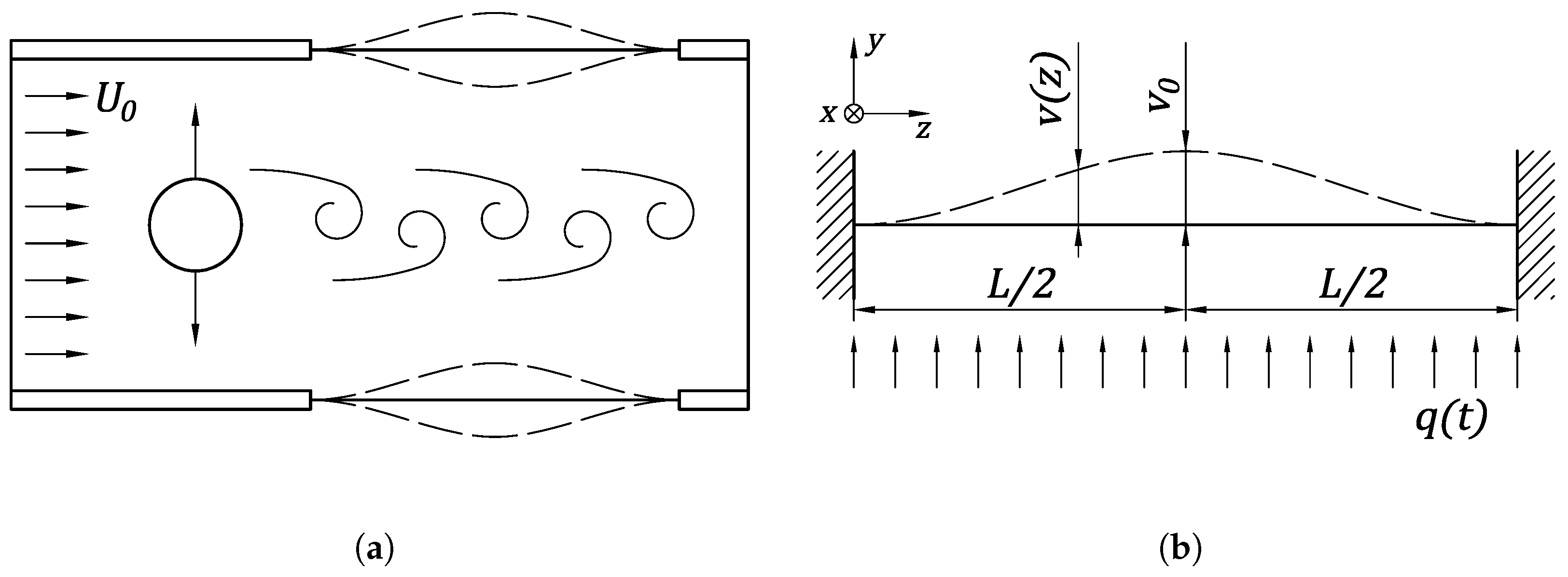
1. Introduction

Despite their high efficiency, traditional hydroelectric plants come with significant drawbacks. In particular, they often require high hydraulic heads, typically achieved through dam construction, which is costly and environmentally disruptive. As a result, the potential for energy extraction from smaller water sources remains largely untapped. In this context, mini- and micro-hydro systems provide a promising alternative. Among these, devices that exploit the Vortex-Induced Vibration (VIV) phenomenon [1,2,3,4,5,6] are notable for their strong performance despite a simple design, effectively addressing the need for affordability and scalability. These systems harness the oscillatory motion caused by the Von Karman vortex street, which consists of a pattern of alternating vortices forming behind a bluff body in a fluid stream. The resulting pressure imbalance induces transverse oscillations in the object, which can be exploited for electricity generation via piezoelectric or electromagnetic mechanisms. When the vortex shedding frequency matches the natural frequency of the body, the so-called “lock-in” condition occurs, amplifying oscillations and enhancing energy conversion.

This concept was first implemented in the VIVACE project [7], whose primary goal was to convert hydrokinetic energy into electrical energy by harnessing the oscillatory motion of a smooth cylinder via an electromagnetic induction generator. Subsequent studies have aimed to improve these devices’ efficiency and power density through novel geometric configurations and enhanced energy conversion mechanisms. In this framework, Zhang et al. [8] arranged four cylinders in a staggered configuration, achieving a power-to-volume density of 133 W/m³. Another enhancement was proposed by Franzini and Bunzel [9], who assessed the effect of an additional degree of freedom (streamwise displacement) on a single-cylinder device’s performance, obtaining an increase of up to three times in energy harvesting efficiency compared to the case of pure transverse displacement. Additional energy extraction can also be achieved by exploiting the Vortex Street-Induced Vibration (VSIV) phenomenon alongside VIVs. This requires the adoption of flexible panels positioned downstream of the bluff body, on which the vortex street exerts a periodic pressure load. The resulting oscillation is then converted into electrical energy using piezoelectric generators [10,11,12,13].

To accurately predict and optimize the performance of these devices, advanced numerical models have been developed. The study of fluid dynamics through advanced numerical models is a well-established approach in different fields, ranging from large-scale industrial applications to micro-scale flow systems [14]. In this context, multiphase fluid dynamics modeling and material removal mechanisms, as studied for example by [15,16,17], can be investigated to understand how the abrasive effects of particles in water might lead to performance degradation in VIV-based energy harvesting devices. Now, shifting the focus to the modeling of the fluid–structure interaction in such systems, Akaydin et al. [10] developed a three-way coupled interaction simulation to study a system where a cantilever flapping sheet was excited by the wake of a smooth transversal cylinder positioned upstream. The simulation was based on a Computational Fluid Dynamics (CFD) analysis, performed in Ansys Fluent^®, integrated with a single-degree-of-freedom (DOF) model representing the structural–electric response. On the other hand, Hu et al. [13] proposed a theoretical three-way coupling model for a similar configuration, where fluid dynamic effects were considered using the Lamb–Oseen vortex model. Notably, in both studies, the structural elastic response was modeled according to the Rayleigh–Ritz method, considering only the first bending mode. This led to a linear, one-dimensional elastic response equation, in accordance with the Euler–Bernoulli linear beam theory. However, this approach is not always feasible. In the present study, we consider a case where additional energy extraction is harnessed from the vibration of two clamped–clamped piezoelectric panels positioned along the channel walls. For simplicity, each plate is approximated as a double-clamped beam subjected to a uniformly distributed transverse load $q\left(t\right)$. However, unlike in the case of a cantilever beam, the applied constraints introduce a so-called geometric non-linearity, as the assumption of negligible mean line elongation becomes inaccurate [18]. This necessitates more complex modeling of the structural elastic response. The effect of geometric non-linearity on the transverse vibration of a clamped–clamped beam was first modeled by Duffing [19], who introduced a cubic restoring force in the classical forced oscillator equation. Several methods have been proposed in the literature to solve the resulting equation of motion. In particular, an analytical approximate solution can be obtained for the undamped case via perturbation and harmonic balance methods [20,21], while cases involving damping require a numerical approach, such as those proposed by Lindfield and Penny [22]. The problem has also been extensively studied using finite element methods (FEMs). In particular, Ribeiro and Petyt [23] employed the hierarchical finite element method (HFEM) and the harmonic balance method (HBM) to analyze the non-linear vibration of a uniform slender beam. In this case, the equations of motion were derived from the principle of virtual work, assuming negligible damping. With HFEM, convergence is achieved with fewer degrees of freedom compared to classical FEM, significantly reducing computational cost. On the other hand, Ribeiro [24] adopted a finite element approach to assess the validity of the Duffing equation, aiming to explain discrepancies between theoretical and experimental evidence. Their findings indicated that neglecting longitudinal damping and in-plane inertia is a necessary assumption for adopting a cubic restoring force. Regarding the theoretical modeling of such a non-linear problem, a key difficulty arises from the fact that models consisting of a single Duffing-like oscillator equation are often inaccurate and unsuitable for capturing phenomena such as internal resonance and the amplitude dependency of the fundamental mode shape. The latter problem, observed experimentally [25], is typically addressed by expressing the steady-state forced response as the sum of at least two modes. Meanwhile, internal resonance results from strong interactions between different modes near a resonant frequency, leading to a multi-modal response [26,27]. Consequently, significant effort has been devoted to characterizing the spatial component of the non-linear harmonic response. Bennouna and White [28] experimentally examined the fundamental mode shape of a clamped–clamped beam at large deflections. They also used the HBM method to solve the beam’s equation of motion, deriving a fourth-order differential equation for the spatial component. The resulting theoretical amplitude dependence of the fundamental mode shape was qualitatively similar to experimental measurements. Similar results were obtained by Benamar et al. [29], who expanded the spatial response into a finite series of even functions of the curvilinear coordinate along the beam’s length. They then derived a set of non-linear algebraic equations of motion through Hamilton’s principle and, by imposing the contribution of a single function, determined the associated non-linear fundamental mode shape. Their results align well with theoretical and experimental observations [28]. A general semi-analytical approach to the non-linear dynamic response problem under free and forced vibration conditions was developed by Azrar et al. [30]. In this study, the authors used Lagrange’s equations to derive a set of non-linear partial differential equations of motion, referred to as the multidimensional Duffing equation. The harmonic balance method was then applied to obtain a set of non-linear algebraic equations in the vibration amplitudes associated with each mode. In this contribution, a single-mode approach was adopted to improve the accuracy of amplitude–frequency relationships for both free and forced vibrations. The general multi-mode approach was subsequently applied in a later work by the same authors [31], where the steady-state forced harmonic response was investigated. It is worth noting that both studies considered undamped vibrations, and further refinements are needed to account for damping effects.

Despite the substantial body of research on the non-linear vibration of clamped–clamped beams, there remains a lack of a simple yet accurate model for describing the structural response in a system that exploits VSIVs to enhance the energy extraction of a VIV-based energy harvester. Such a model is crucial for designing an efficient device, where the primary objective is to maximize displacement amplitude to enhance energy extraction while ensuring structural integrity. The present study aims to address this gap by developing an energy-based model that accounts for the correlation between mode shape and displacement amplitude. Notably, the choice of an energy-based approach is due to its versatility with respect to classical non-linear dynamic models. This enables one to consider a variable shape function, while maintaining a single-degree-of-freedom model. The approach begins by characterizing the variability of the shape function through interpolation of results obtained from static structural FEM simulations. The elastic response of the beam is then described under quasi-static deformation conditions by equating external work to the elastic energy accumulated in large deflection scenarios. These results enable the formulation of a dynamic equilibrium algebraic equation, which is solved using the Newton–Raphson algorithm. To validate the proposed model, its accuracy in capturing the beam’s structural response is evaluated under static conditions. Additionally, its ability to predict response amplitudes is assessed by comparing its results with transient structural FEM analyses. Notably, the model assumes that the excitation frequency is significantly lower than the beam’s first linear natural frequency, simplifying the analysis by avoiding complexities associated with internal resonance. Moreover, it is important to specify that this study focuses exclusively on the structural dynamics of the system, aiming to develop a structural model suitable for integration into a three-way coupling algorithm, which is essential for a comprehensive description of VIV and VSIV energy harvesting. Consequently, the piezoelectric patches on the plate, which play a crucial role in converting mechanical motion into electrical energy, are not considered in the present analysis. Likewise, the fluid–structure interaction driving the oscillatory motion is approximated using a time–harmonic load.

Here is a breakdown of the structure of the current document: In Section 2, the purposes and derivation of the semi-analytical model are accurately described. At this stage, after a formal definition of the problem, the adopted assumptions are specified. In Section 3, the results of each model are compared to those of Structural Simulations performed in Ansys^®, whose reliability is assessed through mesh and time-step sensitivity analyses. The dependency of the model’s error on the adopted assumptions is the object of an in-depth discussion. Finally, in Section 4, the characteristics of the proposed models are summarized and the principal results are highlighted.

2. Materials and Methods

In the energy-harvesting device under investigation, two flexible plates are positioned downstream of the oscillating cylinder and their vibration is driven by a periodic pressure load caused by the vortex shedding from the cylinder. The transversal edges of each plate are fixed to the channel walls, assumed rigid, yielding a clamped–clamped constraint condition. A scheme of the system under investigation is illustrated in Figure 1a.

The global effect of the water in the channel can be described as a pressure load that varies with time, t, and position on the plate’s surface. Assuming a periodic signal with a single dominant frequency, the pressure signal can be approximated as follows:

$$p\left(t\right)=p_{0}sin\left(\omega t\right)$$

(1)

where $p_0$ is the amplitude and $\omega$ is the pulsation of the pressure wave. Since the fixed constraints are applied only at two opposite edges of the plate, it is convenient to model it as a clamped–clamped beam, aligned along the z-axis, represented in Figure 1b. In the resulting two-dimensional model, the pressure signal $p\left(t\right)$ yields a uniformly distributed load $q\left(t\right)=wp\left(t\right)$, where w represents the width of the beam. The consequent beam’s dynamic displacement in y-direction, denoted $v_d$, is a function of time and the z-coordinate. To capture this dependency, we assume a stationary wave solution [29] in the form

$$v_d(z,t)=v(z,v_{0,d})sin(\omega t+{\varphi }_0)$$

(2)

where ${\varphi }_0$ represents the initial phase of the harmonic time-dependent factor, while $v(z,v_{0,d})$ is the spatial component, which is a function of z and of the dynamic mid-span displacement amplitude, $v_{0,d}$, used as a reference value. In this contribution, an energetic approach, inspired by the Rayleigh quotient method, is adopted to estimate the characteristic displacement amplitude in both static and dynamic conditions, denoted $v_{0,s}$ and $v_{0,d}$, respectively. This is conducted under the assumption of excitation frequencies sensibly smaller than the first linear natural frequency of the beam, which allows the definition a priori of a shape function $v(z,v_0)$.

2.1. Elastic Energy Estimation

The total elastic energy, U, accumulated in the beam can be expressed as a function of the characteristic displacement amplitude $v_0$, once the shape function $v(z,v_0)$ is defined. This is valid under both static and dynamic deformation conditions, for which the characteristic displacement is denoted by $v_{0,s}$ and $v_{0,d}$, respectively. Specifically, this energy is given by the integral of the elastic energy density, $e_p$, over the beam’s volume, V:

$$U(v_0)={\int }_V{e}_p(\overrightarrow{P},v_0)dV$$

(3)

where $\overrightarrow{P}$ indicates a generic point in the beam. According to the generalized Hooke’s law, being the stress field $\overrightarrow{\sigma }$ uniaxial and oriented along the z-axis, the elastic energy density is given by

$$e_p={\displaystyle \frac{{\sigma }_z^2}{2E}}$$

(4)

where E is the Young modulus of the material and ${\sigma }_z$ represents the stress component in z-direction, given by Hooke’s law:

$${\sigma }_z=E{ϵ}_z$$

(5)

where ${ϵ}_z$ denotes the strain’s z-component. According to [18], the latter is expressed as the sum of two terms, denoted ${ϵ}_b$ and ${ϵ}_a$, due to bending and stretching, respectively. According to this subdivision, Equation (5) becomes

$${\sigma }_z=E\left({ϵ}_a+{ϵ}_b\right)$$

(6)

that, by multiplying the Young’s modulus by both the strain components, can be rewritten as

$${\sigma }_z={\sigma }_a+{\sigma }_b$$

(7)

The axial bending stress, ${\sigma }_b$, is distributed along the y-axis following Navier’s law. By using the elastic deflection equation, which relates the bending moment to the beam’s curvature, the following equation is obtained:

$${\sigma }_b=-Ey{\displaystyle \frac{d^{2}v}{d{z}^2}}$$

(8)

On the other hand, ${\sigma }_a$ is associated with the elongation of the mean line, ${ϵ}_a$. By neglecting any displacement component except that in the y-direction, $v(z,v_0)$, we obtain [18]

$${\sigma }_a\simeq E{\displaystyle \frac{1}{2}}{\left({\displaystyle \frac{dv}{dz}}\right)}^2$$

(9)

The stress ${\sigma }_z$ in Equation (4) is now expanded by substituting Equations (8) and (9) into Equation (7). This makes explicit the dependency of the elastic energy density on the adopted shape function $v(z,v_0)$, which is denoted as v for brevity:

$$e_p={\displaystyle \frac{1}{2}}E\left[{\displaystyle \frac{1}{4}}{\left({\displaystyle \frac{dv}{dz}}\right)}^4+y^2{\left({\displaystyle \frac{d^{2}v}{d{z}^2}}\right)}^2-y{\left({\displaystyle \frac{dv}{dz}}\right)}^2{\displaystyle \frac{d^{2}v}{d{z}^2}}\right]$$

(10)

This expression is replaced into Equation (3) and, after some algebra, the total stored elastic energy can be expressed as

$$U={\displaystyle \frac{1}{2}}E{\int }_0^L\left[{\displaystyle \frac{1}{4}}A{\left({\displaystyle \frac{dv}{dz}}\right)}^4+I_x{\left({\displaystyle \frac{d^{2}v}{d{z}^2}}\right)}^2\right]dz$$

(11)

where A and $I_x$ denote the area and the second moment of area of the beam’s cross-section, respectively, while L represents the beam’s length. Here, U depends on the first and second derivatives of the displacement distribution $v(z,v_0)$, the geometrical properties of the beam (A, $I_x$), and the elastic properties of the material (E). In order to write the elastic energy as a function of the characteristic displacement $v_0$, the displacement distribution $v(z,v_0)$ must be mathematically defined. According to the beam’s linear theory, for the considered constraint configuration, the shape function is expressed as a fourth-order polynomial:

$$v(z,v_0)={\displaystyle \frac{16v_0}{L^4}}{z}^2{(L-z)}^2$$

(12)

This expression accurately reproduces the shape function observed when $v_0$ is small and the non-linear effects are limited. The implications of this choice will be discussed in Section 3.2. By substituting this expression, Equation (11) can be solved analytically, yielding

$$U={\displaystyle \frac{1}{2}}E\left[{\displaystyle \frac{2·{16}^{4}A{v}_0^4}{15015L^3}}+{\displaystyle \frac{{32}^2{I}_x{v}_0^2}{5L^3}}\right]$$

(13)

This expression is subdivided into two terms: the first, proportional to $v_0^4$, represents the contribution from the mean line elongation, while the second term, proportional to $v_0^2$, corresponds to the bending contribution. Therefore, Equation (13) shows the non-linear effect of the mean line elongation. This aspect will be the object of a more detailed discussion in the next section.

2.2. Quasi-Static Deformation

In this section, the static structural behavior of the beam is investigated. The main purpose of this is to define a characteristic stiffness $k_0$, associated with $v_0$. This will enable us to make some considerations on the problem’s non-linearity. Consider the quasi-static deformation of the beam under a uniformly distributed static load, which is slowly increased up to its maximum value, q. By neglecting any form of dissipation, since inertial effects are not influential in this case, the deformation progresses until the total work done by the external load is balanced by the elastic energy accumulated within the beam. This equilibrium condition can be expressed as follows:

$$W(v_{0,s},q)=U\left(v_{0,s}\right)$$

(14)

where $v_{0,s}$ denotes the characteristic displacement under static equilibrium conditions. To compute the work W, the beam’s stiffness is initially assumed to be constant. In this case, we can write

$$W(v_0,q)={\displaystyle \frac{1}{2}}{\int }_0^{L}qv(z,v_0)dz$$

(15)

By substituting $v(z,v_0)$ from Equation (12), the integral can be solved analytically, yielding

$$W(v_0,q)={\displaystyle \frac{1}{2}}qL{\displaystyle \frac{16}{30}}{v}_0$$

(16)

Therefore, the energetic equivalence of Equation (14) is rewritten using Equations (13) and (16), both evaluated at static equilibrium ($v_0\equiv v_{0,s}$):

$$E\left[{\displaystyle \frac{2·{16}^{4}A{v}_{0,s}^4}{15015L^3}}+{\displaystyle \frac{{32}^2{I}_x{v}_{0,s}^2}{5L^3}}\right]=qL{\displaystyle \frac{16}{30}}{v}_{0,s}$$

(17)

It is now possible to define the characteristic stiffness, $k_0$, representative of the beam’s elastic properties:

$$k_0:={\displaystyle \frac{qL}{v_0}}$$

(18)

According to Equation (17), the following expression is derived for the value of $k_0$ at static equilibrium, denoted as $k_{0,s}$:

$$k_{0,s}={\displaystyle \frac{30}{16}}E\left[{\displaystyle \frac{2·{16}^{4}A{v}_{0,st}^2}{15015L^3}}+{\displaystyle \frac{{32}^2{I}_x}{5L^3}}\right]$$

(19)

Note that the stiffness $k_{0,s}$ in Equation (19) depends on $v_{0,s}^2$, which contradicts the initial hypothesis of the constancy of the stiffness. Therefore, to maintain consistency, the definition of external work must be adjusted accordingly. To simplify the procedure, the beam is replaced with a structure consisting of n nodes connected by springs, which replicate the elasticity of the original body. A scheme of the considered structure is reported in Figure 2.

The displacement and load functions, $v(z,v_0)$ and $q\left(z\right)=q$, are now represented by n-dimensional vectors: $\overrightarrow{v}\left(v_0\right)$ and $\overrightarrow{q}$. Therefore, the structural elastic response is given by

$$\overrightarrow{q}=\left[K\right]\overrightarrow{v}$$

(20)

where $\left[K\right]$ is an $n\times n$ stiffness matrix. As a result, the external work for the continuum beam is expressed as

$$W=\underset{n\to \infty }{lim}\left({\int }_0^{\overrightarrow{v}}{\overrightarrow{v}}^T\left[K\right]d\overrightarrow{v}\right)$$

(21)

Since, for Equation (12), the displacement distribution $v(z,v_0)$ is directly proportional to $v_0$, we define $\overrightarrow{v^{\ast }}:=\overrightarrow{v}\left(v_0\right)/v_0$. Similarly, we assume that the stiffness matrix can be expressed as $\left[K\right]=\left[K^{\ast }\right]k_0$, where the characteristic stiffness $k_0$, defined in Equation (18), is the only term dependent on $v_0$. Thus, Equation (21) becomes

$$W=\underset{n\to \infty }{lim}\left({\overrightarrow{v^{\ast }}}^T\left[K^{\ast }\right]\overrightarrow{v^{\ast }}{\int }_0^{v_0}{v}_0{k}_{0}d{v}_0\right)$$

(22)

The functional correlation between $k_0$ and $v_0$ is assumed according to Equation (19):

$$k_0=a{v}_0^2+b$$

(23)

where a and b are constants. Therefore, by substituting into Equation (22) and analytically solving the integral, we obtain

$$W={\displaystyle \frac{1}{2}}\underset{n\to \infty }{lim}\left[{\overrightarrow{v^{\ast }}}^T\left[K^{\ast }\right]\overrightarrow{v^{\ast }}\left({\displaystyle \frac{1}{2}}a{v}_0^2+b\right)v_0^2\right]$$

(24)

The definition of a coefficient $\gamma :={\displaystyle \frac{\frac{1}{2}a{v}_0^2+b}{a{v}_0^2+b}}$, yields

$$W={\displaystyle \frac{1}{2}}\underset{n\to \infty }{lim}\left({\overrightarrow{v^{\ast }}}^T\left[K^{\ast }\right]\overrightarrow{v^{\ast }}\gamma k_{0,s}{v}_{0,s}^2\right)$$

(25)

In static equilibrium, the external load is balanced by the elastic force: $\overrightarrow{q}=\left[K^{\ast }\right]\overrightarrow{v^{\ast }}{k}_{0,s}{v}_{0,s}$. Thus, by substituting into Equation (25), the external work at equilibrium, denoted $W_s$, becomes

$$W_s={\displaystyle \frac{1}{2}}\underset{n\to \infty }{lim}\left({\overrightarrow{v^{\ast }}}^T\overrightarrow{q}\gamma v_{0,s}\right)$$

(26)

Since the load q is uniformly distributed along the beam, Equation (26) can be rewritten as

$$W_s={\displaystyle \frac{1}{2}}q\gamma {\int }_0^{L}v(z,v_{0,s})dz$$

(27)

This integral, except for the constant $\gamma$, is equivalent to that of Equation (15), yielding

$$W_s={\displaystyle \frac{1}{2}}qL\gamma v_{0,s}{\displaystyle \frac{16}{30}}$$

(28)

By defining a non-linearity parameter $\mathrm{\Gamma }:={\displaystyle \frac{a{v}_0^2}{b}}$, the corrective coefficient $\gamma$ can be expressed as

$$\gamma ={\displaystyle \frac{1}{2\left[1+{\left(\mathrm{\Gamma }\right)}^{-1}\right]}}+{\displaystyle \frac{1}{1+\mathrm{\Gamma }}}$$

(29)

where $\mathrm{\Gamma }$ is the ratio of the elastic energy due to membrane effects (arising from mean line elongation) to that associated with bending (remember the considerations in Equation (13)). By comparing Equations (23) and (19), the values of a and b in its definition are computed, yielding

$$\mathrm{\Gamma }={\displaystyle \frac{10·{16}^{4}A{v}_0^2}{{32}^2·15015I_x}}$$

(30)

Before introducing the corrected $W_s$ in a new definition of the characteristic stiffness $k_0$, it is worth considering another aspect. Specifically, until now, we accepted the definition of a fourth-order polynomial shape function (Equation (12)) as an assumption. However, several contributions [23,28,29] highlighted that the mode shapes of a clamped–clamped beam are amplitude-dependent. For this reason, the choice of a single, constant, shape function appears imprecise, even for static deformation. However, the most suitable shape function to be employed in these cases is not obvious. Benamar et al. [29] observed that, as the displacement increases, the bending modes of a double-clamped beam approach those of a hinged–hinged configuration. Therefore, the displacement distribution of a linear beam under this type of constraint is considered:

$$v(z,v_0)={\displaystyle \frac{4v_0}{L}}\left(z-{\displaystyle \frac{z^2}{L}}\right)$$

(31)

This parabolic shape function, when substituted into Equation (27) and the integral is solved, yields the same result as Equation (28) where we obtain ${\displaystyle \frac{4}{6}}$ instead of ${\displaystyle \frac{16}{30}}$. In general, we can write

$$W_s={\displaystyle \frac{1}{2}}qL\gamma v_{0,s}\beta$$

(32)

where $\beta$ varies in the range $0.53÷0.67$ as $\mathrm{\Gamma }$ increases. To empirically characterize its variability, a parametric analysis of the beam’s shape function is performed. Specifically, among the considered parameters, we express the dimensions of the beam as ratios of its length, $w/L$ and $s/L$, where w and s are the beam’s width and thickness, respectively; on the other hand, the pressure is normalized to a characteristic value, $\tilde{p}$, dependent on the properties of the beam:

$$\tilde{p}:={\displaystyle \frac{E}{1000}}{(s/L)}^2$$

(33)

where, for structural steel, the Young modulus is $E=2·{10}^{11}$ Pa. Thanks to this definition, for a given ratio $p/\tilde{p}$, the obtained displacement magnitude is comparable in a wide range of beam thicknesses. For each parameter, an array of possible values is defined.

Table 1. Parameters’ arrays.

Parameter	Lower Bound	Upper Bound	Number of Elements
$w/L$	$0.5$	$1.5$	3
$s/L$	$0.001$	$0.01$	10
$p/\tilde{p}$	$0.5$	5	4

reports the bounds and the length of these arrays:

Each parameter combination defines an individual for which a static structural FEM analysis is performed in Ansys Mechanical. The reliability of these simulations is assessed through a mesh sensitivity analysis, presented in

Table 2. Mesh sensitivity analysis.

Upper Bound Geometry
Mesh refinement	Number of elements	$v_{0,s}\left[m\right]$	${\eta }_{v,s}[\%]$	$U\left[J\right]$	${\eta }_U[\%]$
Coarse	800	9.122$·{10}^{-3}$	−0.023	77.226	−0.082
Mean	2622	9.126$·{10}^{-3}$	0.012	77.310	0.026
Fine	6000	9.126$·{10}^{-3}$	0.012	77.332	0.055
Lower Bound Geometry
Mesh refinement	Number of elements	$v_{0,s}\left[m\right]$	${\eta }_{v,s}[\%]$	$U\left[J\right]$	${\eta }_U[\%]$
Coarse	800	5.931$·{10}^{-3}$	−0.024	0.1279	−0.052
Mean	2622	5.933$·{10}^{-3}$	0.008	0.1280	0.016
Fine	6000	5.933$·{10}^{-3}$	0.015	0.1280	0.036

. The resulting displacement distribution along the z-axis, referred to as the beam’s mean line, is compared to that corresponding to a quartic shape function (Equation (12)), and the root-mean-square ($rms$) error is normalized to that of a parabolic displacement distribution. Figure 3 reports the normalized $rms$ deviation, denoted ${\xi }_q$, plotted towards the parameter $\mathrm{\Gamma }$.

When $\mathrm{\Gamma }$ is low, the non-linear effects are less influential and the actual displacement distribution tends to the quartic shape function, which is theoretically exact in the linear case. Differently, for high values of $\mathrm{\Gamma }$, the elongation of the mean line becomes dominant and the $rms$ deviation increases asymptotically. The edge case of ${\xi }_q=1$ corresponds to a parabolic shape function. Simulation data can be regressed by an analytical function, $g\left(\mathrm{\Gamma }\right)$, defined as

$$g\left(\mathrm{\Gamma }\right)={\displaystyle \frac{2}{\pi }}arctan\left(c_1{\mathrm{\Gamma }}^{c_2}\right)$$

(34)

where the most suitable values of $c_1$ and $c_2$ are found to be $c_1=0.354$ and $c_2=0.633$, leading to a global $rms$ error, with respect to all the regressed points, of $0.19\%$. Therefore, in our calculations, the tendency of the beam to show a parabolic shape function instead of a quartic one is quantified, within the interval $[0,1]$, by the function $g\left(\mathrm{\Gamma }\right)$. In particular, this result is employed to assume the trend of $\beta \left(\mathrm{\Gamma }\right)$ between its extreme values ($16/30$ and $4/6$):

$$\beta \left(\mathrm{\Gamma }\right)=\left({\displaystyle \frac{4}{6}}-{\displaystyle \frac{16}{30}}\right)g\left(\mathrm{\Gamma }\right)+{\displaystyle \frac{16}{30}}$$

(35)

Since the coefficient $\beta$ can now be computed using Equation (35), it is possible to derive a more accurate correlation for $k_{0,s}$. To achieve this, we replace Equations (13) and (32) with the energetic equivalence of Equation (14), obtaining

$${\displaystyle \frac{1}{2}}qL\gamma v_{0,s}\beta ={\displaystyle \frac{1}{2}}E\left[{\displaystyle \frac{2·{16}^{4}A{v}_{0,s}^4}{15015L^3}}+{\displaystyle \frac{{32}^2{I}_x{v}_{0,s}^2}{5L^3}}\right]$$

(36)

Regarding the elastic energy, U, correcting its expression to account for the shape function variability would require more detailed modeling of the strain field to ensure accuracy. Therefore, Equation (13) is maintained to satisfy the requirement for a simple model. An in-depth discussion on the accuracy in estimating the elastic energy is presented in Section 3.2. From Equation (36), according to the definition of $k_0$ (Equation (18)), the following expression is derived for the stiffness at static equilibrium, $k_{0,s}$:

$$k_{0,s}={\displaystyle \frac{1}{\beta }}E{\displaystyle \frac{1}{\gamma }}\left[{\displaystyle \frac{2·{16}^{4}A{v}_{0,s}^2}{15015L^3}}+{\displaystyle \frac{{32}^2{I}_x}{5L^3}}\right]$$

(37)

It is worth specifying that $\beta$ and $\gamma$ are functions of the parameter $\mathrm{\Gamma }$, which depends on the characteristic displacement $v_0$. So assuming a functional correlation between $k_0$ and $v_0$ as in Equation (37) leads to an approximate model for the stiffness–displacement correlation. This means that further iterations on $W_s$ and $k_{0,s}$ could be performed to improve the model. Moreover, only the terms inside brackets, in Equation (37), correspond to a Duffing-type stiffness, while the presence of $\beta$ and $\gamma$ introduces a higher-order correlation between characteristic stiffness ($k_0$) and displacement ($v_0$). This incongruence can be traced back to both the employment of a variable shape function in computing $W_s$ and the adoption of a constant shape function in the computation of the elastic energy, U.

Since we now dispose of an approximate equation for $k_{0,s}$, it is possible to define a simple iterative algorithm for the estimation of the static displacement $v_{0,s}$ under a given load q. On this purpose, the estimate at step i, denoted $v_{0,s}^{\left(i\right)}$, is employed to compute the corresponding stiffness $k_{0,s}^{\left(i\right)}$ and the displacement is updated at the step $i+1$. An under-relaxation factor R is introduced to enhance convergence:

$$v_{0,st}^{(i+1)}=R{\displaystyle \frac{qL}{k_{0,st}^{\left(i\right)}}}+(1-R)v_{0,st}^{\left(i\right)}$$

(38)

In this process, the static displacement computed with the linear beam’s theory is taken as an initial guess, $v_{0,s}^{\left(1\right)}$. For the upcoming analyses, an over-relaxation factor of 0.5 will be adopted.

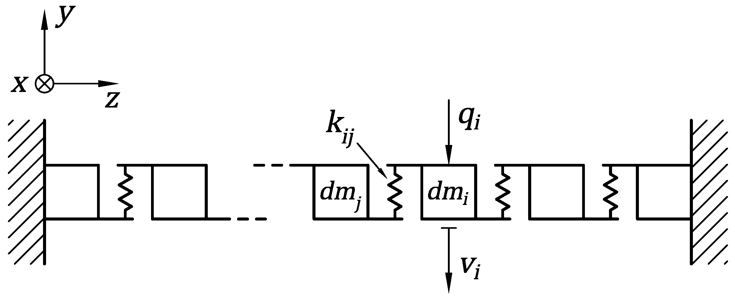
2.3. Dynamic Deformation

In this section, the effect of a harmonically oscillating distributed load, $q\left(t\right)$, is analyzed. Under this load, the dynamic displacement, $v_d(\overrightarrow{P},t)$, is assumed to be described by the stationary wave function of Equation (2). In this case, two parameters must be determined, $v_0$ and ${\varphi }_0$, where the presence of an initial phase arises from the non-negligible effect of a damping coefficient c. The unknowns can be computed by numerically solving the Duffing equation associated with the characteristic displacement $v_0$. For this purpose, the coefficients of mass, damping and non-linear stiffness can be determined through an energetic integral approach, as carried out by Benamar et al. [29]. However, in this study, another approach is adopted in order to take into account the variability of the shape function, which is not feasible with a single Duffing-like equation. Moreover, this approach grants a better handling of the effect of damping, which imposes a complex numerical resolution when using a direct dynamic approach. Specifically, we aim at the description of dynamic equilibrium conditions by two energy equivalences:

• The total energy introduced by the load q over a complete cycle, denoted $W_{q,tot}$, is balanced by viscous dissipation, $W_{c,tot}$.
• The maximum elastic energy, $U_{max}$, is equal to the sum of the maximum kinetic energy, $K_{max}$, and the work done by external and viscous forces from $t_1=-{\varphi }_0/\omega$ to $t_2=t_1+\pi /2\omega$, denoted $W_q$ and $W_c$, respectively.

These conditions yield a system of non-linear equations whose solution can be computed using the Newton–Raphson algorithm. To define an expression for any of the energetic contributions, the assumption of a shape function, $v(z,v_0)$, is required. For the hypothesis of small excitation frequencies, as compared to the first linear natural frequency of the beam, we assume the displacement distributions under static and dynamic conditions to be coincident. Therefore, the same second- and fourth-order polynomials of Section 2.2 can be employed and the shape function’s dependence on the parameter $\mathrm{\Gamma }$ is described by $g\left(\mathrm{\Gamma }\right)$ (Equation (34)). This implies that, for the maximum elastic energy, $U_{max}$, Equation (13) is still valid, when the characteristic displacement $v_0$ corresponds to the dynamic displacement amplitude, $v_{0,d}$. On the other hand, the total kinetic energy at time t is given by

$$K\left(t\right)={\displaystyle \frac{1}{2}}\rho A{\int }_0^L{\dot{v}}_d^2(z,t)dz$$

(39)

where L is the beam’s length, A denotes its cross-sectional area, $\rho$ is the density of the material, and the instantaneous velocity distribution ${\dot{v}}_d(z,t)$ is computed as the first time derivative of the displacement function $v_d(z,t)$, defined in Equation (2):

$${\dot{v}}_d(z,t)=\omega v(z,v_{0,d})cos(\omega t+{\varphi }_0)$$

(40)

Substituting Equation (40) into Equation (39) and solving the integral for both the adopted shape functions yields

$$K\left(t\right)={\displaystyle \frac{1}{2}}\rho A{v}_{0,d}^2{\omega }^2\delta \left(\mathrm{\Gamma }\right)Lco{s}^2(\omega t+{\varphi }_0)$$

(41)

where $\delta \left(\mathrm{\Gamma }\right)$ varies from the extreme value corresponding to a fourth-order polynomial shape function, equal to ${16}^2/630$, to that of a second-order polynomial, $16/30$, as $\mathrm{\Gamma }$ increases. In particular, its trend towards $\mathrm{\Gamma }$ is assumed, similarly to $\beta \left(\mathrm{\Gamma }\right)$, to be defined by the interpolating function $g\left(\mathrm{\Gamma }\right)$ introduced in Equation (34):

$$\delta \left(\mathrm{\Gamma }\right)=\left({\displaystyle \frac{16}{30}}-{\displaystyle \frac{{16}^2}{630}}\right)g\left(\mathrm{\Gamma }\right)+{\displaystyle \frac{{16}^2}{630}}$$

(42)

Notably, for dynamic deformation, the parameter $\mathrm{\Gamma }$ is time-dependent due to the presence of the characteristic displacement $v_0\left(t\right)$ in its definition (Equation (30)). Therefore, it is possible to write the time-dependent formulation of $\mathrm{\Gamma }$ as follows:

$$\mathrm{\Gamma }={\displaystyle \frac{10·{16}^{4}A{v}_{0,d}^2}{{32}^2·15015I_x}}si{n}^2(\omega t+{\varphi }_0)$$

(43)

where, in accordance with Equation (2), the time-dependent characteristic displacement $v_0\left(t\right)$ has been expressed as $v_0\left(t\right)=v_{0,d}sin(\omega t+{\varphi }_0)$. Although this aspect has been neglected for the quasi-static case, in this section, its effects may be relevant and we must account for them. In the computation of $K_{max}$, however, the time-dependency of $\delta$ is not considered, although it could imply that the maximum kinetic energy is achieved when the cosine squared does not equal 1. Due to this simplification, the value of $\delta$ associated with $K_{max}$ corresponds to ${16}^2/630$, since the characteristic displacement in this condition is $v_0=0$. This yields the following expression for the maximum kinetic energy:

$$K_{max}={\displaystyle \frac{1}{2}}\rho A{v}_{0,d}^2{\omega }^2{\displaystyle \frac{{16}^2}{630}}L$$

(44)

For the power associated with viscous dissipation, its instantaneous value is given by

$$P_c\left(t\right)={\int }_0^L{q}_c(z,v_{0,d},t){\dot{v}}_d(z,v_{0,d},t)dz$$

(45)

where the distributed load due to damping, $q_c$, depends on the damping coefficient c, and the displacement velocity ${\dot{v}}_d$:

$$q_c(z,v_0,t)=-c{\dot{v}}_d(z,v_{0,d},t)$$

(46)

Although other formulations of the damping load are possible, Equation (46) is adopted to model the viscous dissipation caused by the surrounding fluid. By solving the integral, we obtain

$$P_c\left(t\right)=-c{v}_{0,d}^2{\omega }^2\delta \left(\mathrm{\Gamma }\right)Lco{s}^2(\omega t+{\varphi }_0)$$

(47)

The energy dissipated over a general time interval $[{\tau }_1,{\tau }_2]$ is given by

$$W_{c,[{\tau }_1,{\tau }_2]}=-c{v}_{0,d}^2{\omega }^{2}L{\int }_{{\tau }_1}^{{\tau }_2}\delta \left(\mathrm{\Gamma }\right)co{s}^2(\omega t+{\varphi }_0)dt$$

(48)

where, as anticipated, the coefficient $\delta \left(\mathrm{\Gamma }\right(t\left)\right)$ is in general time-dependent. For simplicity, instead of $\delta$ into the integral, we consider its average value in the interval $[{\tau }_1,{\tau }_2]$, denoted ${\overline{\delta }}_{[{\tau }_1,{\tau }_2]}$, which is constant and can be computed numerically:

$$\begin{array}{cc}\hfill {\overline{\delta }}_{[{\tau }_1,{\tau }_2]}& ={\displaystyle \frac{1}{{\tau }_2-{\tau }_1}}{\int }_{{\tau }_1}^{{\tau }_2}\delta \left(\mathrm{\Gamma }\left(t\right)\right)dt\hfill \end{array}$$

(49)

$$\begin{array}{cc}\hfill & ={\displaystyle \frac{1}{{\tau }_2-{\tau }_1}}{\int }_{{\mathrm{\Gamma }}_1}^{{\mathrm{\Gamma }}_2}\delta \left(\mathrm{\Gamma }\right)\left({\displaystyle \frac{dt}{d\mathrm{\Gamma }}}\right)d\mathrm{\Gamma }\hfill \end{array}$$

(50)

Therefore, Equation (48) is approximated by

$$W_{c,[{\tau }_1,{\tau }_2]}=-c{v}_{0,d}^2{\omega }^{2}L{\overline{\delta }}_{[{\tau }_1,{\tau }_2]}{\int }_{{\tau }_1}^{{\tau }_2}co{s}^2(\omega t+{\varphi }_0)dt$$

(51)

The error associated with this approximation has been computed for the parameter set presented in Table 1, considering 10 possible frequencies, uniformly distributed from $1$ Hz to $5$ Hz, and 5 possible phase angles ${\varphi }_0$, from 0 to $-\pi$. It emerges that the magnitude of the maximum deviation arising from the adoption of a constant value for $\delta$ equals $4\%$, both for the cases of integration over an entire cycle and over the first fourth of a cycle. The energy dissipated over an entire cycle, $W_{c,tot}$, is computed by setting ${\tau }_1=-{\varphi }_0/\omega$ and ${\tau }_2={\tau }_1+2\pi /\omega$, yielding

$$W_{c,tot}=-c{v}_{0,d}^2{\omega }^2{\overline{\delta }}_1\left(\mathrm{\Gamma }\right)L{\displaystyle \frac{\pi }{\omega }}$$

(52)

On the other hand, by setting ${\tau }_2={\tau }_1+\pi /2\omega$, the energy dissipated during the first fourth of the cycle is obtained:

$$W_c=-c{v}_{0,d}^2{\omega }^2{\overline{\delta }}_2\left(\mathrm{\Gamma }\right)L{\displaystyle \frac{\pi }{4\omega }}$$

(53)

Notably, the mean values ${\overline{\delta }}_1\left(\mathrm{\Gamma }\right)$ and ${\overline{\delta }}_2\left(\mathrm{\Gamma }\right)$ each refer to the relative time interval $[{\tau }_1,{\tau }_2]$. Finally, the power introduced by $q\left(t\right)$ corresponds to

$$P_q\left(t\right)={\int }_0^{L}q\left(t\right){\dot{v}}_d(z,v_0,t)dz$$

(54)

where the external load is given by $q\left(t\right)=q_{0}sin(\omega ,t)$. Thus, by substituting the integrand terms, Equation (54) becomes

$$P_q\left(t\right)=q_0\omega sin\left(\omega t\right)cos(\omega t+{\varphi }_0){\int }_0^{L}v(z,v_0)dz$$

(55)

Here, except for the constants, the integral is analogous to that of Equation (15) ($W_s$), and its solution yields

$$P_q\left(t\right)=q_0{v}_{0,d}\omega sin\left(\omega t\right)cos(\omega t+{\varphi }_0)\beta \left(\mathrm{\Gamma }\right)L$$

(56)

Similar to Equation (48), the work done by the external load over the time interval $[{\tau }_1,{\tau }_2]$ is computed as

$$W_{q,[{\tau }_1,{\tau }_2]}=q_0{v}_{0,d}\omega L{\int }_{{\tau }_1}^{{\tau }_2}\beta \left(\mathrm{\Gamma }\right)sin\left(\omega t\right)cos(\omega t+{\varphi }_0)dt$$

(57)

and, as for $\delta$, the coefficient $\beta \left(\mathrm{\Gamma }\right(t\left)\right)$ is made time-independent by considering its average value, ${\overline{\beta }}_{[{\tau }_1,{\tau }_2]}$. For the estimation of the associated error, in order to avoid possible perturbations occurring when the integral of Equation (57) is null, we refer to the error in computing

$${\int }_{{\tau }_1}^{{\tau }_2}\beta \left(\mathrm{\Gamma }\left(t\right)\right)\left|sin\left(\omega t\right)cos(\omega t+{\varphi }_0)\right|dt$$

(58)

For the same parameter set, excitation frequencies, and phase angles tested for $\delta$, the magnitude of the maximum deviation associated with the adoption of a constant value for $\beta$ equals $3\%$ when the domain of integration is an entire cycle and $4.5\%$ for integration over the first fourth of a cycle. Despite the errors associated with this procedure, the adoption of ${\overline{\delta }}_{[{\tau }_1,{\tau }_2]}$ and ${\overline{\beta }}_{[{\tau }_1,{\tau }_2]}$ is necessary to express the dynamic equilibrium in the form of an algebraic equation in the variables $v_{0,d}$ and ${\varphi }_0$. Through analytical integration, Equation (57) yields the total energy introduced over an entire cycle:

$$W_{q,tot}=-q_0{v}_{0,d}\omega {\overline{\beta }}_1\left(\mathrm{\Gamma }\right)L{\displaystyle \frac{sin\left({\varphi }_0\right)\pi }{\omega }}$$

(59)

Similarly, the energy introduced during the first fourth of a cycle $W_q$, corresponds to

$$W_q=q_0{v}_{0,d}\omega {\overline{\beta }}_2\left(\mathrm{\Gamma }\right)L\left[-{\displaystyle \frac{cos\left({\varphi }_0\right)}{4\omega }}cos\left(2{\varphi }_0\right)-{\displaystyle \frac{sin\left({\varphi }_0\right)\pi }{4\omega }}+{\displaystyle \frac{sin\left({\varphi }_0\right)}{4\omega }}sin\left(2{\varphi }_0\right)\right]$$

(60)

Each term of the dynamic equilibrium condition is now mathematically defined. In order to solve the consequent system of equations, it is convenient to rewrite it as follows:

$$F\left({\underline{x}}_d\right)=\underline{0}$$

(61)

where ${\underline{x}}_d$ is defined as ${\underline{x}}_d:=\left\{\begin{array}{c}{v}_{0,d}\hfill \\ {\varphi }_0\hfill \end{array}\right\}$, being $v_{0,d}$ and ${\varphi }_0$ the amplitude and initial phase of the displacement function, respectively. Meanwhile, the function $F:{\mathbb{R}}^2\to {\mathbb{R}}^2$ corresponds to

$$F\left(\underline{x}\right):=\left\{\begin{array}{c}{W}_{q,tot}(v_{0,d},{\varphi }_0)+W_{c,tot}\left(v_{0,d}\right)\\ K_{max}\left(v_{0,d}\right)+W_q(v_{0,d},{\varphi }_0)+W_c\left(v_{0,d}\right)-U_{max}\left(v_{0,d}\right)\end{array}\right\}$$

(62)

The i-th step of the Newton–Raphson method is

$${\underline{x}}^{(i+1)}={\underline{x}}^{\left(i\right)}+{[\nabla F]}^{-1}F\left({\underline{x}}^{\left(i\right)}\right)$$

(63)

where the Jacobian matrix $[\nabla F]$ can be derived analytically. In particular, the first derivative of ${\overline{\delta }}_{[{\tau }_1,{\tau }_2]}$ in $v_{0,d}$ is computed as

$$\begin{array}{cc}\hfill {\displaystyle \frac{d}{d{v}_{0,d}}}{\overline{\delta }}_{[{\tau }_1,{\tau }_2]}& ={\displaystyle \frac{d}{d{v}_{0,d}}}\left[{\displaystyle \frac{1}{{\tau }_2-{\tau }_1}}{\int }_{{\tau }_1}^{{\tau }_2}\delta \left(\mathrm{\Gamma }\right)dt\right]\hfill \end{array}$$

(64)

$$\begin{array}{cc}\hfill & ={\displaystyle \frac{1}{{\tau }_2-{\tau }_1}}{\int }_{{\tau }_1}^{{\tau }_2}{\displaystyle \frac{d\delta }{d\mathrm{\Gamma }}}{\displaystyle \frac{d\mathrm{\Gamma }}{d{v}_{0,d}}}dt\hfill \end{array}$$

(65)

Here, the characteristic displacement in the definition of $\mathrm{\Gamma }$, according to Equation (2), is given by $v_0=v_{0,d}sin(\omega t+{\varphi }_0)$. The same procedure is adopted for the derivative of ${\overline{\beta }}_{[{\tau }_1,{\tau }_2]}$ and the integrals are computed numerically.

It is worth specifying that the method is sensible to the initial condition, ${\underline{x}}^{\left(1\right)}$. In particular, the procedure could converge to the trivial solution (${\underline{x}}_d=\underline{0}$) if the first-try displacement amplitude, $v_0^{\left(1\right)}$, is too small. To avoid this issue, the most suitable approach consists of characterizing the function $F\left(\underline{x}\right)$ and its derivatives via simple grid-sampling. However, for our purposes, it is sufficient to take the static displacement amplitude deriving from the linear beam’s theory, which gives considerable overestimation, as an initial guess. On the other hand, the initial phase component is less influential, and thus, we can set ${\varphi }_0^{\left(1\right)}=0$.

3. Results and Discussion

In this section, the accuracy of the proposed model is investigated under both static and dynamic conditions. Specifically, the predictions of stored elastic energy, U, and static displacement, $v_{0,s}$, are compared with results from static structural FEM simulations conducted in Ansys Mechanical. In this framework, an in-depth analysis of the energy estimation’s accuracy is also performed. Finally, the dynamic displacement function $v_d\left(t\right)$, as estimated by the presented model, is compared to the results obtained from a set of transient structural analyses. All the reported data refer to structural steel, characterized by the following mechanical properties: Young’s modulus $E=2·{10}^{11}$ Pa; Poisson ratio $\nu =0.3$; shear modulus $G={\displaystyle \frac{E}{2(1+\nu )}}=7.69·{10}^{10}$ Pa; density $\rho$ = 7850 kg/m ${}^3$. The present analysis accounts for the influence of the most relevant parameters. In particular, these are the dimensions of the plate (L, w, s) and the pressure applied to its surface, p (or the pressure amplitude $p_0$ in the case of a harmonic load). To maintain generality, it is convenient to refer to normalized values. For this purpose, the plate dimensions are expressed by their ratio to the length, L, for which a value of 1 m is adopted in the simulations. Moreover, the pressure is expressed as $p/\tilde{p}$, where the definition of $\tilde{p}$ is reported in Equation (33). Each parameter is varied within the upper and lower bounds of Table 1. Since these bounds correspond to those adopted in the definition of $g\left(\mathrm{\Gamma }\right)$ (Section 2.2), they yield a value of $\mathrm{\Gamma }$ approximately varying in an interval $]0,20[$. This ensures the investigation of the model’s accuracy in scenarios dominated by either bending or membrane effects.

In the following subsections, a sensitivity analysis for mesh and time-step refinement is presented to assess the reliability of the numerical simulations. Then, the mentioned comparative analysis is presented.

3.1. Simulation Refinement Sensitivity

The primary output of the model, under static conditions, is an estimate of the static displacement, $v_{0,s}$. Additionally, the stored elastic energy for a given characteristic displacement, $U\left(v_0\right)$, is a relevant parameter. Since the latter is independent of the loading condition (whether static or harmonic), reference values for both quantities can be obtained using static structural analyses, conducted in Ansys Mechanical. This approach achieves a significant reduction in the computational cost by exploiting the symmetry properties of the plate. In this way, only one quarter of the actual structure needs to be solved. A mesh sensitivity investigation is performed for this type of numerical simulation, adopting two different geometries, characterized by each geometrical parameter fixed at either its lower or upper bound. In both cases, the applied pressure corresponds to $p/\tilde{p}=5$, representing the most critical condition. Three meshes with an increasing number of elements are tested and their results, in terms of $v_{0,s}$ and U, are listed in Table 2. In addition, the corresponding deviations from average values, denoted ${\eta }_{v,s}$ and ${\eta }_U$, respectively, are reported.

The extremely low variability in simulations’ results across different mesh refinements is indicative of good reliability. Therefore, to optimize computational costs, the coarsest mesh is adopted for subsequent simulations. The deformed mesh and the applied boundary conditions are shown in Figure 4.

In order to employ the same mesh in the transient structural analyses presented in Section 3.3, a new sensitivity analysis is performed. The same three meshes of the previous case are tested in a transient analysis considering the mean geometry and the most critical pressure amplitude ($p_0/\tilde{p}=5$). The adopted time discretization is characterized by 20 samplings per period of the harmonic load. The resulting displacement amplitudes, $v_{0,d}$, are reported in

Table 3. Mesh sensitivity analysis for transient simulations (10 periods at $f=5$ Hz).

Mean Geometry
Mesh Refinement	Number of Elements	${\mathbf{v}}_{\mathbf{0},\mathbf{d}}\left[\mathbf{m}\right]$	${\mathbf{\eta }}_{\mathbf{v},\mathbf{d}}[\%]$
Coarse	800	10.213$·{10}^{-3}$	−0.022
Mean	2622	10.217$·{10}^{-3}$	0.010
Fine	6000	10.217$·{10}^{-3}$	0.012

, along with their deviation from average, denoted as ${\eta }_{v,d}$.

Given the extremely low variability of the results, the coarsest mesh is also employed in transient structural analyses. On the other hand, in this dynamic case, the sensibility for time-step refinement remains to be investigated. For this purpose, three time discretizations with increasing resolution are tested on the mean geometry under the most critical loading condition ($p_0/\tilde{p}=5$). The resulting displacement amplitudes, $v_{0,d}$, are reported in

Table 4. Time-step sensitivity analysis (10 periods at $f=5$ Hz).

Mean Geometry
Time-Step Refinement	Number of Samplings	${\mathbf{v}}_{\mathbf{0},\mathbf{d}}\left[\mathbf{m}\right]$	${\mathbf{\eta }}_{\mathbf{v},\mathbf{d}}[\%]$
Coarse	14	10.243$·{10}^{-3}$	0.102
Mean	20	10.213$·{10}^{-3}$	−0.192
Fine	40	10.242$·{10}^{-3}$	0.09

, along with their deviation from average, ${\eta }_{v,d}$. Notably, the time refinement is defined by the number of samples taken within a single period of the harmonic load. This makes the analysis frequency independent.

The simulations appear to be almost independent of time-step refinement. However, to avoid convergence issues, the mean time-discretization is adopted.

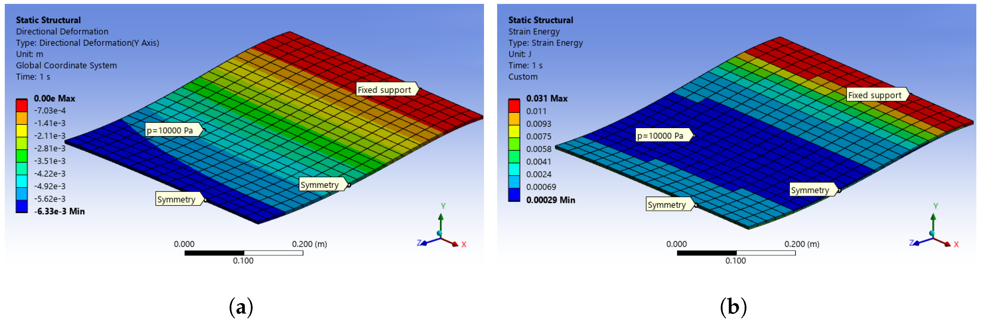
3.2. Accuracy in Static Conditions

In Figure 5, for static loading conditions, the characteristic displacement $v_{0,s}$ and elastic energy estimates $U_s$ are plotted as functions of a single varying parameter, either $s/L$ or $p/\tilde{p}$, while keeping the other parameter fixed at its mean value. From Equation (23), given the definition of the distributed load $q=pw$, we observe that the static displacement should be independent of $w/L$. Although this simplification derives from the adoption of a beam model to represent the plate, good agreement is observed with the simulations’ results. Therefore, for clarity, in Figure 5a,b, the value of $v_{0,s}$ from FEM analyses is reported as the mean value over three different plate widths ($w/L=[0.5;1;1.5]$).

The simplified model shows good adherence to the structural analyses’ results for the investigated conditions, with the exception of Figure 5b, where a maximum relative error of $4.5\%$ is achieved as $s/L$ approaches its upper bound. To further evaluate the performance of the model, a detailed analysis of the deviation from FEM results, as the dominant resistance mechanism varies, is conducted. The relative errors in estimating $v_{0,s}$ and $U_s$, denoted ${\xi }_{v,s}$ and ${\xi }_{U,s}$, respectively, are computed for all the combinations of the parameter arrays in Table 1. These results are plotted in Figure 6 as functions of $\mathrm{\Gamma }$, which express the dominance of the stretching phenomenon over bending. In these graphs, the effect of $w/L$ on the model’s error can also be observed.

It emerges that, as the stretching phenomenon becomes more relevant, the characteristic displacement $v_{0,s}$ is underestimated, while for small values of $\mathrm{\Gamma }$, a sensible overestimation occurs. Moreover, the elastic energy at static equilibrium, $U_s$, shows a similar trend since it is proportional to $v_{0,s}$. The reason for this variability lies in a poor estimation of the energetic terms in Equation (14). Figure 7a reports the estimates of W and U as functions of the characteristic displacement $v_0$, based on the mean parameter set. It emerges that, if the actual $v_{0,s}$ is larger than estimated, this can depend on either an underestimation of $U\left(v_0\right)$ or an overestimation of $W\left(v_0\right)$. The contrary is valid when $v_{0,s}$ is smaller than estimated. Therefore, to justify the trend of Figure 6a, we expect the error on $U\left(v_0\right)$, denoted ${\xi }_U$, to increase with $\mathrm{\Gamma }$ and that of $W\left(v_0\right)$, represented by ${\xi }_W$, to show an opposite trend. This is confirmed by Figure 7b, where the relative errors are plotted against $\mathrm{\Gamma }$.

From Figure 7b, we observe that ${\xi }_U$ is sensibly affected by the plate width, while ${\xi }_W$ is almost independent of it. This difference can be traced back to the adoption of a beam model. Indeed, although the displacement distribution is almost constant along the plate width, the actual stress field in the plate is not one-directional, as we assumed in the beam, and this reflects on the elastic energy $U\left(v_0\right)$. Moreover, it emerges that the error in estimating the external work is almost null for small values of $\mathrm{\Gamma }$, while ${\xi }_U$ reaches its maximum negative value. This is in contrast with the fact that Equation (13) sticks exactly to the linear beam theory when the stretching energy is neglected. Therefore, further investigation is needed on the accuracy in estimating $U\left(v_0\right)$. Consider two plates, both with $L=w/L=1$ and normalized pressure $p/\tilde{p}=5$. The first plate has thickness $s/L=0.001$ and the other $s/L=0.01$. The parameter $\mathrm{\Gamma }$ in the two cases is $0.429$ and $17.864$, respectively. By analyzing the relative strain fields and elastic energy predictions, some interesting conclusions can be drawn. In this framework, the adoption of a fourth-order polynomial shape function to compute $U\left(v_0\right)$, independently of $\mathrm{\Gamma }$, is justified. Specifically, for both cases, static structural analyses are employed to derive the maximum bending strain and the elongation of the mean line as functions of the z-coordinate, denoted as ${ϵ}_b^{\ast }\left(z\right)$ and ${ϵ}_a^{\ast }\left(z\right)$, respectively. Moreover, by using the obtained y-directional displacement, $v\left(z\right)$, the theoretical mean line elongation, represented by ${ϵ}_{a,v}\left(z\right)$, is computed. In Figure 8, these curves are compared to those relative to second- and fourth-order polynomial shape functions. Notably, the plots are relative to the interval $z\in [0,L/2]$ to enhance clarity.

From Figure 8a,b, we observe that, as membrane effects become dominant, the bending strain ${ϵ}_b^{\ast }\left(z\right)$ tends to that of a parabolic shape function, with the exception of the beam’s extremities, where a considerable deviation is observed. This is due to the increase in the curvature near the clamps for high values of $\mathrm{\Gamma }$, which cannot be captured by the adopted parabolic shape since it assumes a constant curvature. Similarly, the mean line strain distribution, ${ϵ}_{a,v}\left(z\right)$, becomes more similar to that of a second-order polynomial shape function as $\mathrm{\Gamma }$ increases. However, in this case, the direct result of numerical simulations, ${ϵ}_a^{\ast }\left(z\right)$, has a sensibly different trend. Since it is approximately constant and equal to the mean value of ${ϵ}_{a,v}\left(z\right)$, the actual elastic energy due to stretching is much lower than estimated, as shown in

Table 5. Energy estimation errors ${}^1$.

$\mathbf{\Gamma }$	${\mathit{U}}_{\mathit{a}}/{\mathit{U}}_{\mathit{b}}$	${\mathit{\xi }}_{\mathit{U},\mathit{b}}^{\mathit{V}}[\%]$	${\mathit{\xi }}_{\mathit{U},\mathit{b}}^{\mathit{Q}}[\%]$	${\mathit{\xi }}_{\mathit{U},\mathit{a}}^{\mathit{V}}[\%]$	${\mathit{\xi }}_{\mathit{U},\mathit{a}}^{\mathit{Q}}[\%]$	${\mathit{\xi }}_{\mathit{U}}^{\mathit{V}}[\%]$	${\mathit{\xi }}_{\mathit{U}}^{\mathit{Q}}[\%]$
0.429	0.300	$-16.136$	$-7.900$	$39.745$	$31.753$	$-5.406$	$-1.015$
17.864	5.123	$-82.409$	$-64.788$	$64.470$	$22.792$	$42.882$	$10.342$

¹ V: variable shape function; Q: quartic polynomial shape function.

. This inaccuracy can be traced back to the adopted strain–displacement relation. In fact, in Equation (9), the assumption is made that the z-directional displacement, $w\left(z\right)$, is null throughout the entire beam. However, from static structural analyses, a non-zero displacement distribution is found for both the investigated configurations, as shown in Figure 9.

By including $w\left(z\right)$ in the computation of ${ϵ}_{a,v}\left(z\right)$, the relative deviation from ${ϵ}_a^{\ast }\left(z\right)$ is reduced from 64.519% to 6.189%, for the case with $\mathrm{\Gamma }=0.429$, and from 73.463% to 3.911% for the case with $\mathrm{\Gamma }=17.864$. Let us consider, now, the possibility of exploiting the function $g\left(\mathrm{\Gamma }\right)$, defined in Equation (34), to take into account the shape function variability in the computation of $U\left(v_0\right)$. As shown in Table 5, this causes an increase in the error in estimating the elastic energies due both to bending and stretching, denoted ${\xi }_{U,b}$ and ${\xi }_{U,a}$, respectively.

In any case, the errors in estimating the single energy contributions are considerable. However, from the last two columns of Table 5, it emerges that by adopting the fourth-order polynomial shape function, independently from $\mathrm{\Gamma }$, higher accuracy is achieved in estimating the global elastic energy U. Another interesting consideration, arising from Figure 8, is that, regarding for what regards the estimation of the bending energy, the parabolic shape function of Equation (31) does not capture the increase in the beam’s curvature near the clamps, which is particularly relevant for large values of $\mathrm{\Gamma }$. Therefore, one possible improvement could derive from the adoption of a higher-order function, such as a sixth-degree polynomial, instead of the parabolic curve for large values of $\mathrm{\Gamma }$. In particular, this would enable us to consider the variability of the shape function in the computation of the elastic energy U, thus reducing the associated error. Moreover, although the effect of $w\left(z\right)$ is not specified in many contributions throughout the literature, it must be considered when defining a more accurate expression for $U\left(v_0\right)$ that accounts for the shape function variability. For this purpose, it is possible to represent $w\left(z\right)$ as a linear combination of odd harmonic functions, whose coefficients can be computed by minimizing the stored elastic energy. However, the definition of a similar method and the investigation of its effectiveness are not the objects of the present work.

In conclusion, the inaccuracies observed in the computation of the elastic energy accumulated by the material can lead to systematic deviation of the estimated response amplitude $v_0$ in both static and dynamic conditions. Moreover, an error in the accumulated elastic energy can lead to an imprecise estimation of the power output of the energy harvesting device. On the other hand, the global error ${\xi }_U^Q$ is smaller than or equal to $10\%$ in a wide range of $\mathrm{\Gamma }$, which can be considered acceptable in the preliminary design phase.

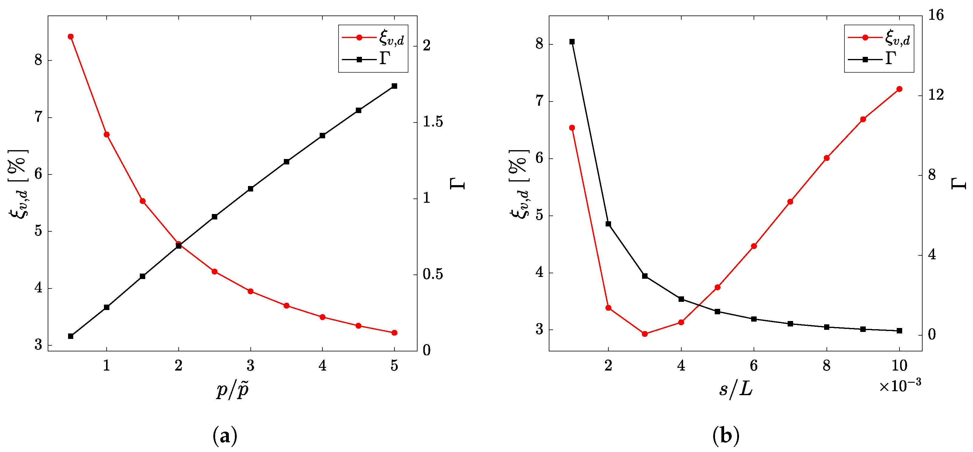
3.3. Accuracy in Dynamic Conditions

In this section, the results of the model in terms of displacement amplitude, $v_{0,d}$, for several dynamic loading conditions, are compared to those obtained through transient structural simulations performed in Ansys Mechanical. Notably, although transient structural simulations require considerable computational costs, their adoption is necessary to take into account the system’s geometric non-linearity, for which harmonic response analyses are not suitable. With reference to Table 1, the normalized thickness is fixed to its mean value, while $s/L$ and $p_0/\tilde{p}$, where $p_0$ denotes the amplitude of the pressure signal, are free to vary between their bounds. Moreover, an array of 10 uniformly distributed frequencies, $f_i$, between $1$ Hz and $5$ Hz is used to define a set of time–harmonic loads, $p_i\left(t\right)=p_{0}sin(2\pi t/f_i)$. Notably, due to the typical vortex shedding frequencies associated with VIV, the investigation of the model’s response with larger excitation frequencies is not necessary. For any combination of parameter set and loading frequency, the time-dependent displacement signal, $v_0\left(t\right)$, from transient structural analysis is decomposed through the FFT algorithm integrated in Matlab^® to obtain the most relevant amplitude, associated with the excitation frequency $f_i$. With this approach, for each parameter set, the response amplitude curve $v_{0,d}\left(f\right)$ is computed in the discrete interval defined by the array of frequencies $\left[f_i\right]$. Regarding damping, according to the classical vibration theory for one-dimensional systems [32,33], we can define the critical damping $c_{cr}$, associated with the clamped–clamped beam under linear conditions, as

$$c_{cr}=2\sqrt{k_{lin}{m}_{eq}}$$

(66)

where $k_{lin}$ is the linear stiffness relative to the transversal displacement of the midpoint of the beam $v_0$, and $m_{eq}$ denotes the equivalent mass associated with the same coordinate. Theoretical integration of the elastic deflection equation yields, for the stiffness $k_{lin}$, the following expression:

$$k_{lin}={\displaystyle \frac{384EI}{L^3}}$$

(67)

where E is the Young modulus of the material, I represents the cross-sectional moment of inertia of the beam, and L denotes its length. On the other hand, in accordance with Equation (44), the equivalent mass is given by

$$m_{eq}=\rho ws{\displaystyle \frac{{16}^2}{630}}L$$

(68)

where $\rho$ represents the density of the material, while w and s denote, respectively, the width and height of the beam’s cross-section. Once the linear critical damping $c_{cr}$ has been computed, it is possible to define the associated damping ratio $\zeta$ as follows:

$$\zeta :={\displaystyle \frac{c}{c_{cr}}}$$

(69)

where c is the damping coefficient. The damping for the investigated configuration is influenced not only by the material properties but also by viscous and dissipative effects arising from energy extraction through piezoelectric patches. Therefore, its magnitude is difficult to estimate in this case. This makes it necessary to assess the accuracy of the model over a wide range of damping conditions. Therefore, a comparison with FEM results is conducted for the two extreme cases: $\zeta =0$ and $\zeta =0.5$. In Figure 10, for the case of $\zeta =0$, the $rms$ relative deviation of the response curves estimated by the proposed model to those obtained through numerical simulations, denoted ${\xi }_{v,d}$, is reported as a function of either $s/L$ or $p_0/\tilde{p}$, while keeping the other parameter fixed at its mean value.

In Figure 11, on the other hand, the same results are presented for the case of $\zeta =0.5$. We can immediately observe the similarity between the curves of Figure 10 and Figure 11, which implies that the accuracy of the model is not sensibly affected by the presence of damping.

In both the investigated damping conditions, it emerges that the error in estimating the displacement amplitude is always smaller than $10\%$. This level of accuracy is acceptable in a preliminary design stage. Moreover, as the parameter $\mathrm{\Gamma }$ increases, the accuracy is enhanced. This trend is disaffected only for small values of the plate thickness, in particular for the case of $\zeta =0$.

4. Conclusions

A simplified model has been proposed for estimating the vibration amplitude of a doubly clamped plate subjected to harmonic pressure over time. With reference to this model, the key findings are summarized below:

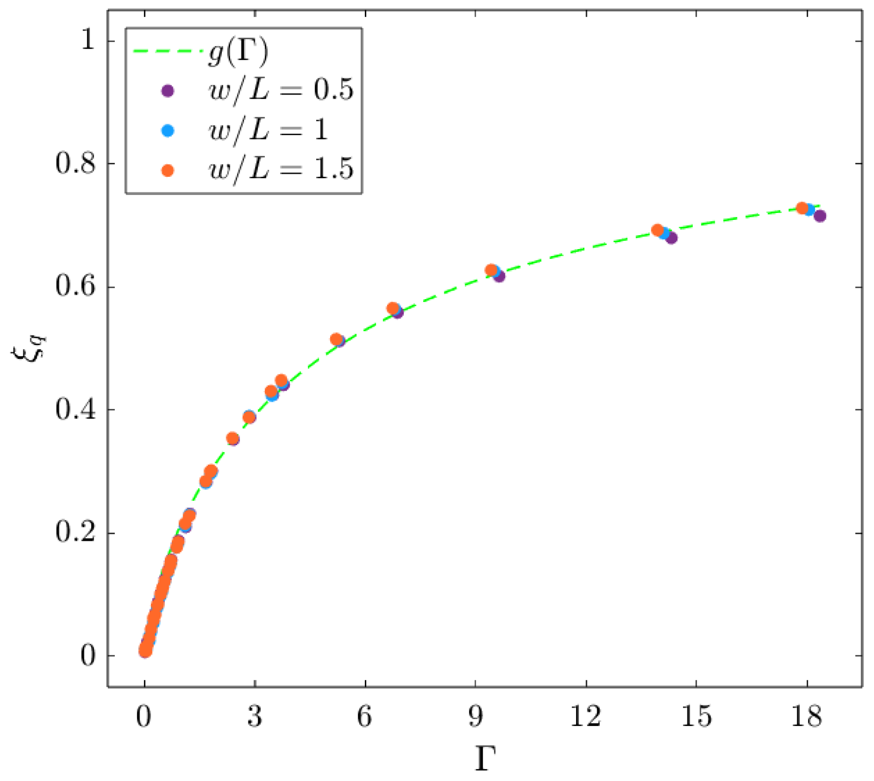
• The variability of the beam’s shape function, under static loading conditions, can be expressed as a function of the parameter $\mathrm{\Gamma }$, which indicates the ratio between the energies associated with membrane and bending effects.
• Under static loading conditions, the proposed model estimates the characteristic displacement, $v_{0,s}$, and the accumulated elastic energy, $U_s$, with an error below $10\%$. This error shows a clear dependence on the non-linearity parameter, $\mathrm{\Gamma }$, the causes of which have been investigated.
• The estimation of potential elastic energy due to bending and stretching effects is characterized by significant errors. However, adopting an invariant shape function expressed as a fourth-degree polynomial allows us to achieve lower errors for the total elastic energy.
• In the case of a time–harmonic pressure load, the error in estimating the response curve of the plate, $v_{0,d}\left(f\right)$, remains below $10\%$ for the examined set of parameters. Once again, the dependence on $\mathrm{\Gamma }$ is evident.

Therefore, the proposed model effectively addresses the problem of estimating the vibration amplitude of the plates in the energy harvester described in the introduction. In particular, the model can be used for the design of the plates once the applied pressure signal is known (which can be obtained, for example, from CFD analysis) and allows for an estimation of the strain energy associated with the plates. The strain energy can be correlated with the deformation of the piezoelectric patches and used to estimate the electrical energy that can be generated by the system, once the efficiency of the piezoelectric patches is known. The accuracy of the proposed model is compatible with a preliminary design stage, while it offers a considerable advantage in terms of simplicity and ease of implementation. On the other hand, the present study highlighted several possible improvements to the proposed approach, which can be implemented in future research. In particular, a more accurate description of the beam’s strain field, which can be achieved through a different choice of the shape functions and by accounting for the effects of the axial displacement field $w\left(z\right)$, would enhance the precision and reliability of the elastic energy computation. Furthermore, incorporating a modal approach would extend the model’s applicability to frequencies close to and even higher than the beam’s first linear natural frequency. This improvement to the model could be useful as it allows the study of conditions closer to resonance, which can be exploited to increase energy extraction from pressure fluctuations. To do this, the Ritz method [34,35] can provide a useful methodological basis. However, due to the typically small values of excitation frequency, this enhancement is considered not essential for the application in the context of VIV-based energy harvesting.

References

- Feng, C. The Measurement of Vortex Induced Effects in Flow Past Stationary and Oscillating Circular and D-Section Cylinders. Ph.D. Thesis, University of British Columbia, Vancouver, BC, Canada, 1968. [Google Scholar] [CrossRef]
- Williamson, C.; Roshko, A. Vortex formation in the wake of an oscillating cylinder. J. Fluids Struct. 1988, 2, 355–381. [Google Scholar] [CrossRef]
- Sarpkaya, T. A critical review of the intrinsic nature of vortex-induced vibrations. J. Fluids Struct. 2004, 19, 389–447. [Google Scholar] [CrossRef]
- Williamson, C.H.; Govardhan, R. Vortex-induced vibrations. Annu. Rev. Fluid Mech. 2004, 36, 413–455. [Google Scholar] [CrossRef]
- American Society of Mechanical Engineers. Eigen-Solution for Flow Induced Oscillations (VIV and Galloping) Revealed at the Fluid-Structure Interface. Volume 2: CFD and FSI. In International Conference on Offshore Mechanics and Arctic Engineering; American Society of Mechanical Engineers: New York, NY, USA, 2019. [Google Scholar] [CrossRef]
- Gabbai, R.; Benaroya, H. An overview of modeling and experiments of vortex-induced vibration of circular cylinders. J. Sound Vib. 2005, 282, 575–616. [Google Scholar] [CrossRef]
- Bernitsas, M.M.; Raghavan, K.; Ben-Simon, Y.; Garcia, E.M.H. VIVACE (Vortex Induced Vibration Aquatic Clean Energy): A New Concept in Generation of Clean and Renewable Energy From Fluid Flow. J. Offshore Mech. Arct. Eng. 2008, 130, 041101. [Google Scholar] [CrossRef]
- Zhang, B.; Mao, Z.; Song, B.; Tian, W.; Ding, W. Numerical investigation on VIV energy harvesting of four cylinders in close staggered formation. Ocean Eng. 2018, 165, 55–68. [Google Scholar] [CrossRef]
- Franzini, G.R.; Bunzel, L.O. A numerical investigation on piezoelectric energy harvesting from Vortex-Induced Vibrations with one and two degrees of freedom. J. Fluids Struct. 2018, 77, 196–212. [Google Scholar] [CrossRef]
- Akaydin, H.D.; Elvin, N.; Andreopoulos, Y. Energy Harvesting from Highly Unsteady Fluid Flows using Piezoelectric Materials. J. Intell. Mater. Syst. Struct. 2010, 21, 1263–1278. [Google Scholar] [CrossRef]
- Weinstein, L.A.; Cacan, M.R.; So, P.M.; Wright, P.K. Vortex shedding induced energy harvesting from piezoelectric materials in heating, ventilation and air conditioning flows. Smart Mater. Struct. 2012, 21, 045003. [Google Scholar] [CrossRef]
- Akaydin, H.; Elvin, N.; Andreopoulos, Y. Wake of a cylinder: A paradigm for energy harvesting with piezoelectric materials. Exp. Fluids 2010, 49, 291–304. [Google Scholar] [CrossRef]
- Hu, Y.; Yang, B.; Chen, X.; Wang, X.; Liu, J. Modeling and experimental study of a piezoelectric energy harvester from vortex shedding-induced vibration. Energy Convers. Manag. 2018, 162, 145–158. [Google Scholar] [CrossRef]
- Li, L.; Xu, P.; Li, Q.; Zheng, R.; Xu, X.; Wu, J.; He, B.; Bao, J.; Tan, D. A coupled LBM-LES-DEM particle flow modeling for microfluidic chip and ultrasonic-based particle aggregation control method. Appl. Math. Model. 2025, 143, 116025. [Google Scholar] [CrossRef]
- Tan, Y.; Ni, Y.; Xu, W.; Xie, Y.; Li, L.; Tan, D. Key technologies and development trends of the soft abrasive flow finishing method. J. Zhejiang Univ. Sci. A 2023, 24, 1043–1064. [Google Scholar] [CrossRef]
- Pandey, A.; Shrestha, S.; Abregu, J.; Nascimben, F.; Chitrakar, S.; Neopane, H.P.; Dahlhaug, O.G. Erosion Induced Flow Changes in Pelton Bucket: A Numerical Approach. IOP Conf. Ser. Earth Environ. Sci. 2024, 1385, 012014. [Google Scholar] [CrossRef]
- Sun, J.; Spinosa, P.; Messa, G.V. Analysis of different strategies for the prediction of hydro-abrasive wear in Pelton turbine buckets based on Computational Fluid Dynamics (CFD) simulations. Wear 2025, 205954. [Google Scholar] [CrossRef]
- Ghuku, S.; Saha, K.N. A review on stress and deformation analysis of curved beams under large deflection. Int. J. Eng. Technol. 2017, 11, 13–39. [Google Scholar] [CrossRef]
- Duffing, G. Erzwungene Schwingungen bei veränderlicher Eigenfrequenz und ihre technische Bedeutung. J. Appl. Math. Mech 1918, 1. [Google Scholar] [CrossRef]
- Hayashi, C. Nonlinear Oscillations in Phisical Systems; Princeton University Press: Princeton, NJ, USA, 1985. [Google Scholar]
- Wilson, J.F. Dynamics of Offshore Structures; Wiley: New York, NY, USA, 1984; pp. 495–519. [Google Scholar]
- Lindfield, G.; Penny, J. Numerical Methods, 4th ed.; Academic Press: New York, NY, USA, 2019; pp. 239–299. [Google Scholar] [CrossRef]
- Ribeiro, P.; Petyt, M. Non-linear vibration of beams with internal resonance by the Hierarchical Finite-Element Method. J. Sound Vib. 1999, 224, 591–624. [Google Scholar] [CrossRef]
- Ribeiro, P. The second harmonic and the validity of Duffing’s equation for vibration of beams with large displacements. Comput. Struct. 2001, 79, 107–117. [Google Scholar] [CrossRef]
- Smith, P.W.J.; Malme, C.I.; Gogos, C.M. Nonlinear Response of a Simple Clamped Panel. J. Acoust. Soc. Am. 1961, 33, 1476–1482. [Google Scholar] [CrossRef]
- Szemplinska-Stupnika, W. The Behaviour of Non-Linear Vibrating Systems; Kluwer Academic Publishers: Dordrecht, The Netherlands, 1990. [Google Scholar]
- Nayfeh, A.H.; Mook, D.T. Nonlinear Oscillations; Wiley: Hoboken, NJ, USA, 1995. [Google Scholar]
- Bennouna, M.; White, R. The effects of large vibration amplitudes on the fundamental mode shape of a clamped-clamped uniform beam. J. Sound Vib. 1984, 96, 309–331. [Google Scholar] [CrossRef]
- Benamar, R.; Bennouna, M.; White, R. The effects of large vibration amplitudes on the mode shapes and natural frequencies of thin elastic structures part I: Simply supported and clamped-clamped beams. J. Sound Vib. 1991, 149, 179–195. [Google Scholar] [CrossRef]
- Azrar, L.; Benamar, R.; White, R. Semi-analytical approach to the non-linear dynamic response problem of S–S and C–C beams at large vibration amplitudes part I: General theory and application to the single mode approach to free and forced vibration analysis. J. Sound Vib. 1999, 224, 183–207. [Google Scholar] [CrossRef]
- Azrar, L.; Benamar, R.; White, R. A semi-analytical approach to the non-linear dynamic response problem of beams at large vibration amplitudes, part II: Multimode approach to the steady state forced periodic response. J. Sound Vib. 2002, 255, 1–41. [Google Scholar] [CrossRef]
- Balachandran, B.; Magrab, E.B. Vibrations; Cambridge University Press: Cambridge, UK, 2018. [Google Scholar]
- Meirovitch, L. Foundamentals of Vibration; McGraw-Hill Education: New York, NY, USA, 2001. [Google Scholar]
- Leissa, A. The historical bases of the Rayleigh and Ritz methods. J. Sound Vib. 2005, 287, 961–978. [Google Scholar] [CrossRef]
- Ritz, W. Über eine neue Methode zur Lösung gewisser Variationsprobleme der mathematischen Physik. J. Fur Reine Angew. Math. 1909, 135, 1–61. [Google Scholar] [CrossRef]