Article

Adaptive Energy Management Strategy for Hybrid Electric Vehicles in Dynamic Environments Based on Reinforcement Learning

1
School of Mechanical and Aerospace Engineering, Jilin University, Changchun 130022, China
2
State Key Laboratory of Advanced Design and Manufacturing Technology for Vehicle, Hunan University, Changsha 410082, China
3
National Key Laboratory of Automotive Chassis Integration and Bionics, Jilin University, Changchun 130025, China
*
Author to whom correspondence should be addressed.
Designs 2024, 8(5), 102; https://doi.org/10.3390/designs8050102
Submission received: 30 August 2024 / Revised: 30 September 2024 / Accepted: 10 October 2024 / Published: 12 October 2024
(This article belongs to the Topic Vehicle Dynamics and Control, 2nd Edition)

Abstract

:
Energy management strategies typically employ reinforcement learning algorithms in a static state. However, during vehicle operation, the environment is dynamic and laden with uncertainties and unforeseen disruptions. This study proposes an adaptive learning strategy in dynamic environments that adapts actions to changing circumstances, drawing on past experience to enhance future real-world learning. We developed a memory library for dynamic environments, employed Dirichlet clustering for driving conditions, and incorporated the expectation maximization algorithm for timely model updating to fully absorb prior knowledge. The agent swiftly adapts to the dynamic environment and converges quickly, improving hybrid electric vehicle fuel economy by 5–10% while maintaining the final state of charge (SOC). Our algorithm’s engine operating point fluctuates less, and the working state is compact compared with Deep Q-Network (DQN) and Deterministic Policy Gradient (DDPG) algorithms. This study provides a solution for vehicle agents in dynamic environmental conditions, enabling them to logically evaluate past experiences and carry out situationally appropriate actions.

1. Introduction

The rapid increase in automobiles, paralleling economic and industrial growth, has heightened environmental pollution concerns [1,2,3]. The hybrid electric vehicle (HEV) is a vital step toward transportation electrification, triggering a shift in the automotive industry from oil dependence to new energy reliance. HEVs primarily aim to enhance power system efficiency and reduce fuel consumption. The energy management strategy (EMS) is one of the pivotal technologies used in HEVs, which can influence fuel consumption significantly, given a specific power system configuration. EMS is classified into rule-based, optimization-based, and learning-based strategies [4,5,6,7].
Rule-based EMS requires formulating control rules for energy distribution under varying driving modes [8,9,10,11,12]. The rule system, although simple to develop, can construct the control system. To address battery limitations, Ding et al. [13] suggested a hybrid strategy for series-parallel plug-in hybrid electric vehicles using rule-based control and genetic algorithm-optimized tactics. Guercioni et al. [14] introduced a distinctive real-time energy management method inspired by optimal solutions for the energy management issue of plug-in hybrid electric vehicles. Mansour et al. [15] created a rule-based energy management strategy, emphasizing real-time calculation for a Prius HEV, and a comprehensive optimization program underpinned by dynamic programming. This optimization process, interconnected with the traffic management system, takes into account the driver’s preferred route via the vehicle’s global positioning system. Notably, the parameters modified by the global optimization algorithm surpass the deterministic rules, proving superior to the rule-based energy management approach. This strategy, however, necessitates substantial processing resources and is typically suited to vehicles on predefined routes, becoming irrelevant when the routes or driving cycles are not pre-known. To remedy these issues, Chen et al. [16] recently introduced a driving pattern recognition method for scrutinizing the vehicle energy management strategy. Lian et al. [17] proposed an enhanced energy management framework by integrating expert knowledge into DDPG. On this premise, Zhou et al. [18] extensively explored and evaluated current driving pattern recognition methods, spotlighting appropriate application scenarios for each predictive algorithm and prospective strategies to handle prediction errors.
Learning-based strategies have gained considerable scholarly attention in recent years. Xu et al. [19] parameterized the key factors in the EMS development process based on reinforcement learning and applied it to the HEV power allocation problem to reduce vehicle fuel consumption. To balance the charge state of multiple-cell batteries in electric vehicles, Chaoui et al. [20] suggested a reinforcement learning-based solution. This extends battery life and reduces the frequency of battery maintenance. Aljohani et al. [21] developed a real-time data-driven routing optimization method for electric vehicles to minimize energy consumption. Zhou et al. [22] utilized reinforcement learning to optimize a hybrid tracked vehicle’s control strategy, with simulation results indicating that the suggested EMS substantially improved fuel efficiency. Xiong et al. [23] benchmarked reinforcement learning against rule-based algorithms. Simulations revealed that the reinforcement learning-based strategy effectively minimized energy loss. Optimizing energy management systems with reinforcement learning faces the challenge of slow convergence due to sparse rewards. To accelerate learning and enhance adaptability, Zhu et al. [24] suggested a hierarchical reinforcement learning approach tailored for energy management strategies. This novel reinforcement learning approach addresses the sparse rewards issue during training and ensures optimal weight distribution.
Moreover, various academics have demonstrated the superior performance of reinforcement learning-based energy management strategies in static environments. Lee et al. [25] employed dynamic programming control methods to compare reinforcement learning strategies. His findings suggest a reinforcement learning policy can attain global optimality in an infinite-horizon optimal control problem—a feat also achievable by stochastic dynamic programming. Aljohani et al. [26] proposed a metadata-driven approach for real-time EV route optimization to reduce road energy demand. Sun et al. [27] proposed the comprehensive energy management method founded on the conventional soft actor critic (SAC) algorithm and prioritized experience to boost training efficiency. Aiming at the problem of computational efficiency and dynamic coordination of energy conversion, Guo et al. [28] proposed a predictive energy management strategy for dual-mode HEV relying on model predictive control (MPC), which exhibits benefit performance and robustness. In complex, static contexts, these notable reinforcement learning approaches have proven their value in energy preservation.
Driving environments are fraught with instability sources, including behavioral biases from wind direction, motion condition changes due to weather, and vehicle part aging, causing shifts in certain physical characteristics [29,30,31,32]. The reinforcement learning agent’s strategy must adapt to environmental dynamics, swiftly adjusting to events diverging from training or changing conditions. Incremental reinforcement learning has recently become the preferred approach to rapid adaptation to dynamic scenarios. As per this concept, the dynamic environment is considered to be a sequence of stationary tasks within a specific timeframe, with each one corresponding to an environmental aspect during the relevant stage. This perspective offers insights for EMS in dynamic settings.
This study proposes an adaptive learning strategy in dynamic environments, allowing the vehicle’s reinforcement learning agent to more logically recall all events and cope with the dynamic environment.
The primary contributions can be outlined as follows:
  • The memory library (ML) comprising specific actions for different driving condition scenarios has been developed for the reinforcement learning agent to leverage.
  • The identification parameters for driving condition blocks and the control parameters in memory library are derived through Dirichlet clustering. During the online process, the control parameters are adjusted by the expectation maximization (EM) algorithm, enabling the agent to continuously build and refine the memory library while retaining previously acquired knowledge.
  • The proposed adaptive learning strategy in dynamic environment (ALDE) algorithm equips the agent with the ability to adapt to changing environments. As the algorithm operates, the agent learns and enhances its capacity for managing a range of normal and extreme driving conditions, constantly.
The remainder of this paper is organized as follows: Section 2 presents the HEV model. Section 3 elaborates on the structure and updates of the ALDE algorithm. Section 4 outlines the verification methodology and results. Section 5 concludes this study.

2. Construction of Vehicle Model

The research focuses on a parallel HEV with a P2 configuration. The P2 HEV model offered by the Matlab/Simulink 2020b community is utilized and modified in the control component to enhance simulation precision and repeatability. Table 1 contains detailed information about the model parameters.

2.1. Vehicle Dynamic Modeling

The power requirement of the vehicle is calculated through the longitudinal force balance equation in Equation (1). The equation is divided into four parts: rolling resistance F f , air resistance F w , ramp resistance F i , and inertial force F a .
F = F f + F w + F i + F a F f = G f F w = 1 2 ρ A f C D v 2 F i = G i F a = δ m a ,
where G represents vehicle gravity, f denotes the rolling resistance coefficient, ρ depicts air density, A f is the front projection area of the vehicle, C D represents the air resistance coefficient, v represents the longitudinal vehicle speed, i represents the road slope (which is 0 in this case, so the term F i can be ignored), δ is the rotational mass conversion coefficient, m represents vehicle mass, and a represents acceleration.
The engine and motor provide the vehicle’s required power, and their relationship is commonly expressed as follows:
P dem = P e n + P b a t η m η T ,
where P e n represents the output power of the engine, P b a t represents the power of the battery, η m represents the efficiency of the motor, and η T represents the transmission efficiency.

2.2. Engine Modeling

The quasi-static model of the engine postulates that parameters such as speed, load, and fuel consumption change gradually over short time intervals, indicating that the engine remains in a state of equilibrium at each time point. This assumption facilitates the use of a simplified equation to characterize the engine’s fuel efficiency and other performance metrics, while excluding the effects of dynamic responses and complex nonlinear behaviors. The fuel consumption rate is expressed as follows:
m ˙ f = f T e n , n e n ,
where T e n is the engine output torque and n e n is the engine speed. The total fuel consumption under one operating cycle can be obtained by the following integrals:
Fuel = t 0 t   m ˙ f d t ,
where t [ t 0 , t ] is the time span of the calculation cycle.

2.3. Motor Modeling

The performance of the motor can be characterized using a power diagram, where motor torque and speed serve as the axes. Rooted in the operating mode of the motor, the following formula is defined:
  P e l e c = 1 η m ω e m , T e m P m e c h = 1 η m ω e m , T e m ω e m T e m if P e l e c 0   ( m o t o r i n g   m o d e ) η m ω e m , T e m P mech = η m ω e m , T e m ω e m T e m if P e l e c < 0   ( g e n e r a t i n g   m o d e ) ,
where P e l e c represents the power of the motor, ω e m represents the speed of the motor, T e m represents the rotation of the motor, η m represents the efficiency of the motor, and P mech represents the mechanical work of the motor.

2.4. Battery Modeling

Power batteries can supply energy to the electric motor as well as store energy generated by the motor. The battery’s SOC is defined by Equation (6):
S O C t = S O C t 0 1 Q b a t t 0 t   I b a t ( t ) d t ,
where I b a t ( t ) represents the battery current and Q b a t represents battery’s rated capacity. If voltage dynamics are ignored and the battery circuit is represented as a RC-free branch, the above formula can be re-expressed as follows:
S O C ˙ = V o c V o c 2 4 R int P b a t 2 R int Q b a t ,
where P b a t represents the battery’s output power, V o c represents the open circuit voltage of the battery, and R int represents the internal resistance of the battery.

3. Adaptive Learning Strategy in Dynamic Environment

3.1. Reinforcement Learning Modeling and Problem Description

Reinforcement learning is mathematically represented as a Markov decision process consisting of five fundamental elements: environment, agent, state, behavior, and reward [33,34,35,36]. It enables an agent to amass the maximum reward value through a reward and punishment mechanism, facilitating autonomous learning in different environments. In this paper, a vehicle’s driving cycle is utilized as the environment that reinforcement learning must navigate. The vehicle controller is an agent of reinforcement learning. The required engine power represents the agent’s action value. The change in engine speed, torque, and battery SOC value is used as the state vector. To address the subjectivity and empirical challenges in traditional reward function design, we propose a strategy grounded in inverse reinforcement learning. The approach derives weights of reward function from expert trajectories, ensuring that the reward function more objectively reflects the balance between fuel efficiency and battery lifespan [37], as follows:
a c t i o n = P e n ,
s t a t e = [ n t ,   T t ,   S O C ] ,
r = t 0 t   α m ˙ f t d t + β SOC t SOC t 0 2 ,
where P e n , n t , T t , and S O C represent engine power output, engine speed, engine torque, and battery SOC, respectively. The reward function consists of two parts. The first term represents fuel consumption; m ˙ f t is the instantaneous fuel consumption rate. The second term represents the difference between initial and current SOC. In Equation (10), α and β are two constant factors.
The dynamic environment of the driving cycle during vehicle operation can be seen as a series of fixed tasks over time. Each task corresponds to specific environmental characteristics relevant to that period. The objective of optimal power allocation is achieved under these environmental conditions, where machine learning (ML) enables the transition from a local optimum to a global optimal fuel consumption. When the vehicle’s driving environment changes, the ALDE algorithm’s agent can initiate a new learning process based on previously acquired knowledge, incrementally adapting it to suit the new conditions. Reinforcement learning agents are akin to the human brain, where changing elements and unexpected disturbances are the norm in real driving scenarios. In contrast, humans possess the necessary driving experience to navigate unforeseen environmental changes. Therefore, enhancing the agent’s adaptability becomes crucial. The key is enabling the agent to compare its own memories and respond promptly. Inspired by human capabilities, we develop ML from which hybrid vehicle agents can draw analogies to effectively handle dynamic environments. This ML must retain historical information to the greatest extent. In this article, an agent’s behavior strategy and the parameters of the dynamic environment are identified as the fundamental elements to be stored in the ML. The ML can be expressed as follows:
M L = X 1 : X 11 X 1 e X 2 : X 21 X 2 f         X i : X i 1 X i j ,     X i j [ ω , p ] i j ,
where X depicts the driving condition block, i demonstrates the number of driving condition clusters, j represents the total number of driving condition blocks in a driving condition cluster, p denotes the dynamic environment, and ω depicts the primary eigenvalue. In this experiment, the number of blocks in the clusters varies depending on the specific cluster.
The dynamic environment parameters can be quantified by the reward function and state vector as follows:
p [ r , s t a t e ] ,
Figure 1 illustrates the proposed algorithmic framework of this paper, which is thoughtfully designed into two main parts: the left side represents the algorithm kernel, while the right side details the vehicle structure. The primary inputs in the present driving condition include the primary eigenvalue ω and the state S, which are fundamental to the ALDE method. The algorithm kernel is divided into two parallel sections. The left side focuses on probability calculations and network training, whose goal is to enhance the responsiveness to environmental changes and intelligence of its decisions. In contrast, the right side emphasizes parameter optimization and iterative updates, ensuring that the vehicle can adapt to changing external conditions while maintaining optimal performance across various operating environments. The parallel processing of these updates significantly enhances the precision and performance of the algorithm. The next A c t i o n computed by the algorithm kernel is then sent to the vehicle structure module for immediate adjustments to the vehicle’s operational behavior, ensuring smooth and safe driving. In summary, the thoughtfully designed structure improves the quality of decisions of the model and adaptability and generalization capabilities in dynamic environments.
Step 1: The first part is to calculate the current aggregation probability so as to determine the driving condition category that the driving condition block belongs to. Meanwhile, the second part performs the DQN algorithm to acquire the optimal action corresponding to this driving cycle block.
Step 2: In the first part, the optimal Action calculated before is recorded in the corresponding ML. It may be used to create a new record, add a working block information record in the existing driving condition, or directly use the control strategy of a working block and use the EM algorithm to update it. The second part also updates the DQN weight through experience playback and turntable transfer.
Step 3: The control closed loop is completed by outputting the Action determined by the present ALDE algorithm.

3.2. Cluster Aggregation in the Adaptive Algorithm

3.2.1. Definition and Characteristics of Driving Condition Block in Cluster Aggregation

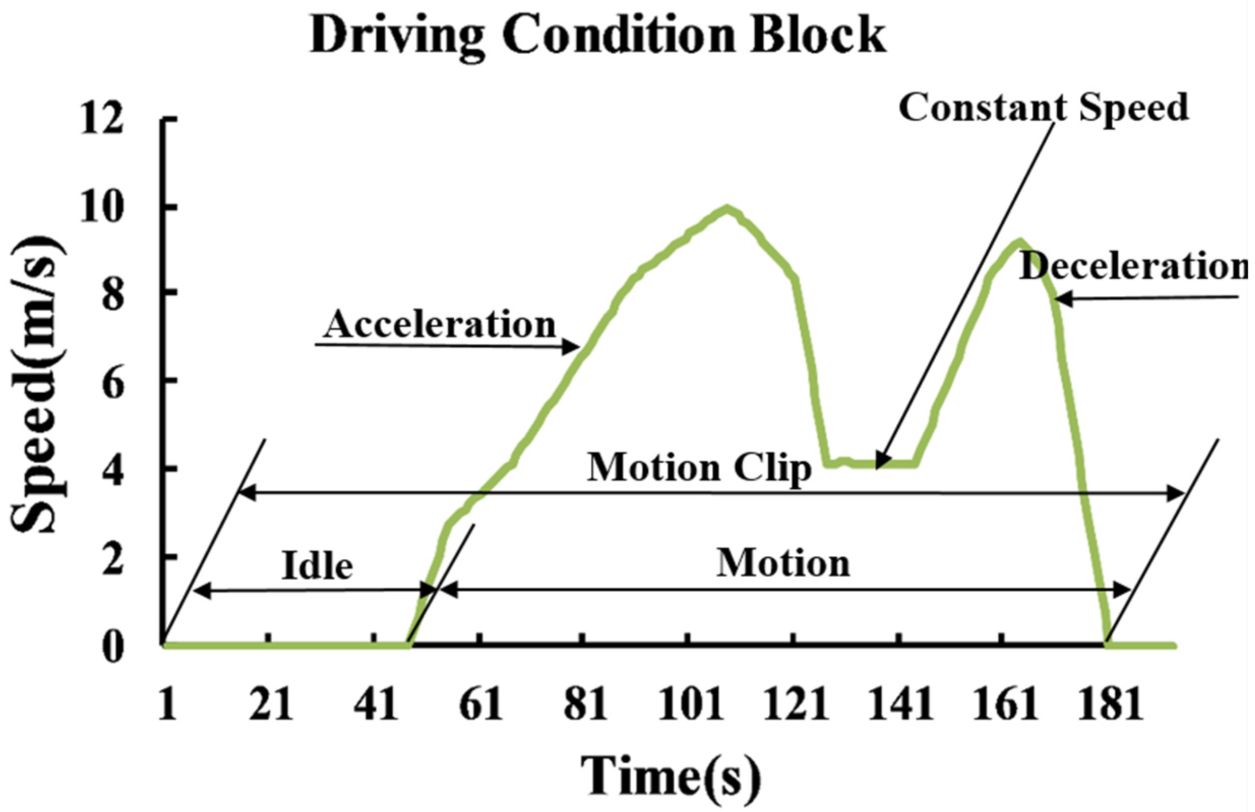
To replicate the frequent start-stop, acceleration, and deceleration of real driving scenarios, we define a driving condition block as the transition between successive idle states. The block generally includes idle segments and dynamic segments. The moving segments typically encompass acceleration, constant speed, and deceleration conditions. Figure 2 depicts the definition of a driving condition block.
Each driving cycle can extract multiple feature parameters. Some characteristics are interconnected and dependent on one another, resulting in repetitive information. Given that feature parameter matrices would be overly complex. Using just one or two arbitrary characteristic parameters may not accurately represent present driving conditions. Therefore, it is crucial to use only the key components to describe the driving conditions and to appropriately limit the dimensions of the matrix.
In this article, 126 blocks are chosen from various standard driving cycles (WLTC, RTS95…) as a training set. The cumulative contribution rate of the first T primary components is
ψ = i = 1 T   λ i i = 1 15   λ i ,
where λ i is the characteristic parameter, ψ represents the cumulative contribution rate of the first T primary components, i = 1 T   λ i denotes the sum of eigenvalues of the first T principal components, and i = 1 15   λ i represents the sum of eigenvalues of the first 15 principal components.
Table 2 shows the specific contribution rate and cumulative contribution rate. Ultimately, three characteristic parameters with the highest contribution rates, average speed, idle time ratio, and working block distance are selected to represent the driving condition block characteristics.

3.2.2. Cluster Aggregation Based on Dirichlet Method

The Dirichlet Process (DP) is a stochastic process characterized by a probability distribution [38,39]. For instance, with a base measure H, the random distribution of DP G can be expressed as G DP α 0 , H , where α 0 is the concentration parameter of DP, which indicates the level of uncertainty in clustering. A lower α 0 value raises the number of clusters, while a higher α 0 value has the opposite effect. H is the basis measure, which is a basic distribution used to represent the cluster center distribution.
The features of every driving cycle type can be represented as a vector X i = X 1 i , , X i j , where X i j is the j driving cycle block feature of the   i driving condition type, and the vector is generated by polynomial distribution with parameters θ 1 i , , θ i j . The activity characteristics of the n driving condition blocks to be clustered form the vector X = X 1 , , X i .
Assume that they are independent of each other and come from a mixed distribution F(Θ), which is composed of multiple polynomial distributions; the parameter Θ that constitutes the probability of variable polynomial distributions can be drawn from DP G DP α 0 , H . If some samples are generated by a mixed distribution under the same parameter Θ , then these data samples can be classified into the same class. The DPMM (Dirichlet Process Mixture Model) that achieves cluster aggregation can be expressed as follows:
x i = X 1 i , , X i j Mult Θ z i , i = 1 , , n ,
Θ = θ z i 1 , , θ z i j Dir β 1 , , β j , 1 z i K ,
z i Mult Π , i = 1 , , n ,
Π = μ 1 , , μ k , , μ K + 1 DP α 0 , H ,
where Equation (14) expresses the block of condition i generated by the polynomial distribution of class z i with parameter θ z i , z i is the class number, and K is the total of classes. Equation (15) indicates the prior distribution of parameter Θ z i , and its parameters are β 1 , , β j . Equation (16) indicates that the z i class is drawn from the polynomial distribution with parameter Π . Equation (17) expresses parameter Π = μ 1 , , μ k , , μ K + 1 , which is extracted from the process G DP α 0 , H .

3.3. Chinese Restaurant Process in ALDE

We propose using the infinite DP mixture model in stochastic dynamic conditions to construct a prior distribution of rising condition clusters, providing a flexible structure for the observed dynamic environment. The Chinese Restaurant Process (CRP) explains this by comparing a sequence of customers sitting at tables in a restaurant, where each table represents a cluster. The likelihood that each customer sits alone at a new table is proportional to the lumped parameter, and the probability that each customer sits at an existing table is related to the number of customers seated here.
The likelihood that characteristics of each working block correspond to an existing class and the probability of belonging to a new class in the Chinese restaurant model are as follows:
μ k = Pr z i = k Z i , X = 1 B n k α 0 + n 1 Pr x i z i = k , 1 k K ,
μ K + 1 = P r z i = K + 1 Z i , X = 1 B α 0 α 0 + n 1 Pr x i z i = K + 1 ,
where k is sample category number X i , B is a normalization factor, which enables the total of probabilities to be 1, n k is the sum of all dimension counts of all samples belonging to class k , and Z i is the set of all classes but z i .

3.4. Adaptive Algorithm Update

To update the adaptive algorithm in a dynamic environment, we propose using the EM algorithm and online Bayesian inference to update the mixed environment model incrementally. The EM algorithm is an iterative optimization algorithm that updates model parameters through the E-step and M-step, aiming to maximize the likelihood function of the model. It is commonly used for parameter estimation in probabilistic models with latent variables. In the E-step, it calculates posterior probabilities of latent variables based on present parameter estimates, typically involving computing expectations. In the M-step, it updates model parameters by maximizing the logarithm of the likelihood function shaped by complete data. This step often involves solving maximization problems. Online Bayesian inference is an inference method used for parameter estimation and prediction in dynamic environments. It involves continuously updating the prior distribution to incorporate new observed data and obtain an approximation of the posterior distribution. In online Bayesian inference, the parameters and states of the model are updated over time. With this approach, the dataset is repetitive as the environment cluster grows larger without sacrificing prior knowledge. When the environment engages with the controller agent, we use ( m , n ) to represent the input and output of the vehicle dynamic environment and ( M t i , N t i ) to represent the input and output at time t. X i t is the present driving condition block, and ω t i is the eigenvalue of the current driving condition block. During each iteration, model parameters are adjusted, leading to an increase in the likelihood function of the probabilistic model with hidden variables. The iteration ends when it no longer rises, or the value of the increase is less than the set threshold. In this section, the EM algorithm is combined with the algorithm to measure the similarity of the vehicle dynamic environment, as follows:
E-Step: The posterior expectation of the present block-to-cluster assignment is
P ω t i M t i , N t i = μ k   , 1 k K μ K + 1 , k = K + 1 ,
Combined with CRP, it can be written as follows:
P ω t i M t i , N t i 1 B n k α 0 + n 1 Pr x i z i = k , 1 k K 1 B α 0 α 0 + n 1 Pr x i z i = k , k = K + 1 ,
M-step: According to the estimated posterior expectation P ω t i M t i , N t i , we execute the M-step to optimize the anticipated log-likelihood arising from the inference environment probability. Assuming that each driving condition begins at the first driving condition block X i 1 , the value of ω t i can be obtained after a gradient update at every stage. The update formula is as follows:
ω t i = ω t 1 i δ t = 1 t 1   P ω t 1 i M t 1 i , N t 1 i ω t 1 i l o g p ω t 1 i N t 1 i M t 1 i ,
where δ is the learning rate of the EM algorithm. We can approximate the formula by incrementally updating the previous parameters in the current environment sample:
ω t i = ω t 1 i δ P ω t 1 i M t 1 i , N t 1 i ω t 1 i l o g p ω t 1 i N t 1 i M t 1 i , i ,
This process avoids the need to store previously observed samples and implements a fully streaming, incremental learning algorithm along with online Bayesian inference. To completely execute the EM algorithm, ALDE needs to switch between the E-step and the M-step repeatedly to achieve convergence. The pseudo-code of ALDE is depicted in Algorithm 1.
Algorithm 1. Pseudo-code of ALDE.
Input: Characteristic parameters of dynamic driving condition blocks
Output: Optimal action (engine power)
1.
Initialize   i = 1 , t = 1
2.
Calculate   the   characteristic   parameters   of   current   driving   condition   block   ω 1 1   and   restore   them   in   the   first   container   of   X 11
3.
Memorize   current   policy   chosen   by   deep   reinforcement   learning   in   the   sec ond   container   of   X 11
4.
for following each driving condition block during one episode do
5.
  Calculate   P ω t i M t i , N t i of current driving condition block and conduct Dirichlet driving condition cluster polymerization
6.
   if   P ω t i M t i , N t i 1 B n k α 0 + n 1 Pr x i z i = k , 1 k K

    Conduct current driving condition block with most resembles action in corresponding
     existing   driving   condition   polymerization   i   and   restore   them   in   the   first   container   of   X i j ,
     the   current   policy   in   the   sec ond   container   of   X i j
7.
else

       Build   a   brand   new   driving   condition   polymerization   i , add current driving
      condition   block   to   this   driving   condition   polymerization   i , and restore them in
       the   first   container   of   X i j ,   the   current   policy   in   the   sec ond   container   of   X i j
8.
  while   ω 1 ~ t i not converging do

     To   update   for   all   previous   time   periods   1 ,   2 ,   , t 1 with:
   ω t i = ω t 1 i δ P ω t 1 i M t 1 i , N t 1 i ω t 1 i log p ω t 1 i N t 1 i M t 1 i , i
9.
end

4. Simulation and Hardware-in-the-Loop Experiment

4.1. Simulation Experiment

To evaluate the effectiveness of the proposed strategy, we assess engine operating points, fuel consumption, and SOC interpolation. We configure the initial state of the vehicle to full gasoline. All algorithms are executed using Python 3.5, running on Ubuntu 16 with 48 Intel(R) Xeon(R) E5-2650 2.20GHz CPU processors, 193GB RAM, and NVIDIA Tesla 32GB GPU.
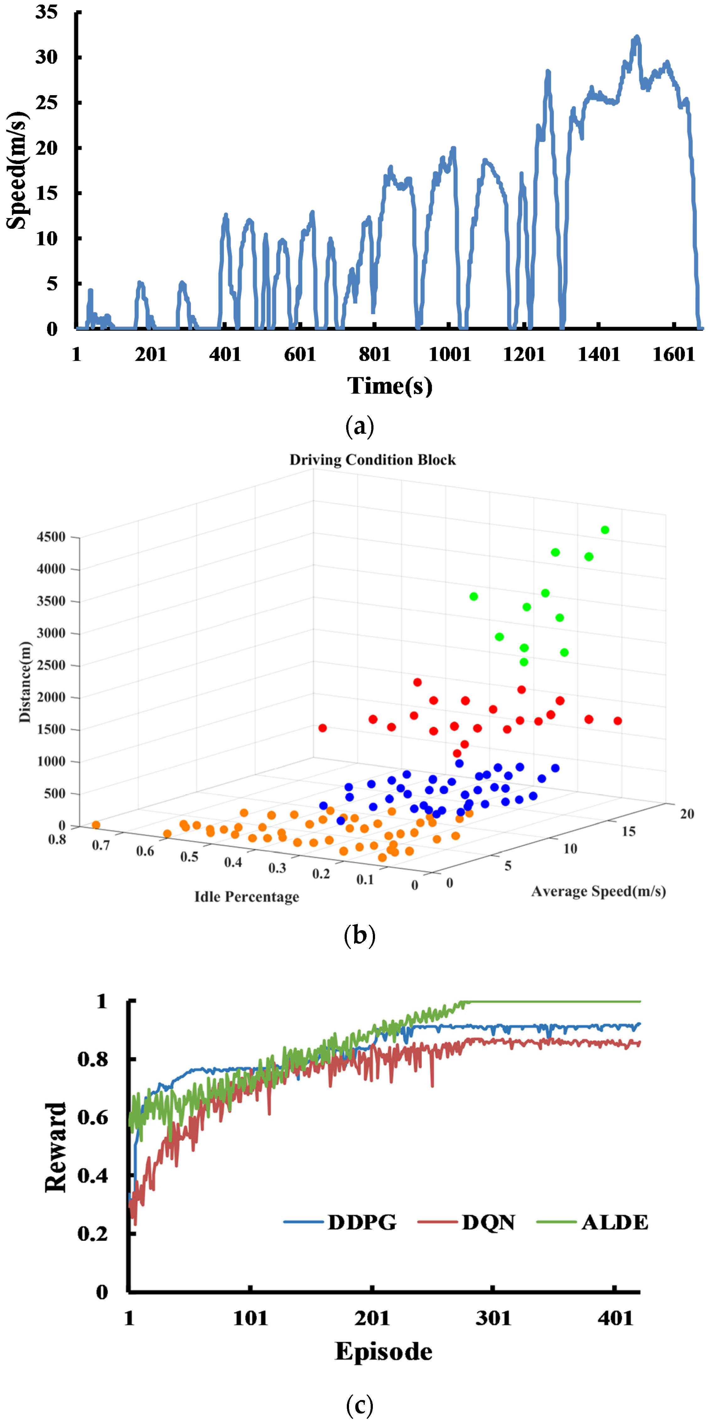
To validate the capability of the ALDE algorithm, we have created a new driving cycle, as shown in Figure 3a. The results of the ML constructed are presented in Figure 3b. The specific types are as follows: (3.505 m/s, 36.27% idle percentage, 198.9 m), (6.781 m/s, 17.82% idle percentage, 687.4 m), (10.02 m/s, 15.85% idle percentage, 1704 m), and (13.51 m/s, 12.80% idle percentage, 3418 m), which are obtained through the Dirichlet clustering method. The scatter points are represented in four colors—orange, blue, red, and green—corresponding to four typical operating conditions. There are four driving conditions within the clustering scenarios: city traffic jam, smooth city traffic flow, suburban area, and highway. City traffic jam refers to a situation where the traffic volume on urban roads is excessively high, resulting in slow and congested vehicle movement. In city traffic jams, vehicles frequently stop, start, and move at low speeds. City smooth traffic flow refers to a situation where the traffic volume on urban roads is relatively stable, allowing vehicles to travel at a moderately steady speed without frequent stops or congestion. Suburban areas typically refer to the outskirts of cities, where traffic volume is relatively low, and roads are wider. In suburban areas, vehicles can usually travel at higher speeds without being affected by city traffic congestion. Highways are road networks designed for high-speed driving. On highways, vehicles can cruise at higher speeds for extended periods, and although traffic volume is relatively high, it is usually smoother. We sequentially train the DQN and DDPG agents on the comprehensive training dataset, which encompasses a variety of driving scenarios, such as LA92, WLTP, RTS95, US06, and more, covering all 126 distinct driving condition clusters as previously mentioned. However, it does not include the new driving cycle. After training the proposed and compared algorithms, their reward curves in new driving condition cycle (test set) are shown in Figure 3c, which demonstrates the convergence speed of three reinforcement learning algorithms under entirely new and unknown driving conditions.
Figure 3c illustrates the reward curve for each iteration of policy iteration in the new driving condition cycle. Compared to DQN and DDPG, our approach demonstrates the quickest adaptation for learning in a dynamic environment and achieves the fastest convergence. This is attributed to its straightforward adaptation mechanism, which effectively leverages learned knowledge from the memory library (ML). Furthermore, the graph indicates that the ALDE algorithm is constantly superior to all baseline methods in terms of return during training, with a relatively stable curve following convergence. This suggests that ALDE provides a more reliable form of adaptation for learning in a dynamic environment. Therefore, the reward function curve illustrates that ALDE is well equipped to handle a dynamic environment where reward or state transition functions may update with each iteration, offering improved adaptation for learning.
DQN and DDPG fail to achieve the ideal standard encountering complete driving conditions that are absent from the training set, which is characteristic of the catastrophic forgetting issue commonly seen in traditional reinforcement learning algorithms. The analysis of the issue is outlined below: After completing comprehensive training on specific driving condition A, the agent experiences a decline in its ability to handle driving condition A when it continues training on a different set of driving condition B. When we extract complete driving conditions from the training set and select specific condition blocks to create a new driving condition for the test set, the DQN and DDPG algorithms encounter the inherent issue of catastrophic forgetting. Additionally, they treat the new complete driving condition as entirely unknown, which needs to be equipped with comprehensive learning.
The ALDE algorithm achieves better performance because of the ability to manage variable driving condition blocks resulting from Dirichlet clustering. It deconstructs the problem into single modules and utilizes the combination of Dirichlet distribution and EM updates. Encountering new driving conditions, the agent attempts to locate the corresponding driving condition sort X i from ML. It then adopts a control strategy of the condition block X i j that is most similar. After achieving the present task, it updates the control strategy of X i j in reverse. To avoid the agent failing to identify the similar driving condition X i , it generates a new condition X i + 1 , updating itself as the X i + 11 . It executes the control strategy from the most similar driving condition block in current ML and updates the strategy for X i + 11 as the process continues. The factors prevent ALDE from forgetting, enabling it to adapt and evolve in entirely new and unknown complete driving conditions. Faced with a new driving condition cycle, ALDE begins with a high initial reward value, which steadily increases as training progresses. After convergence, ALDE has the highest reward value and the smallest fluctuation.
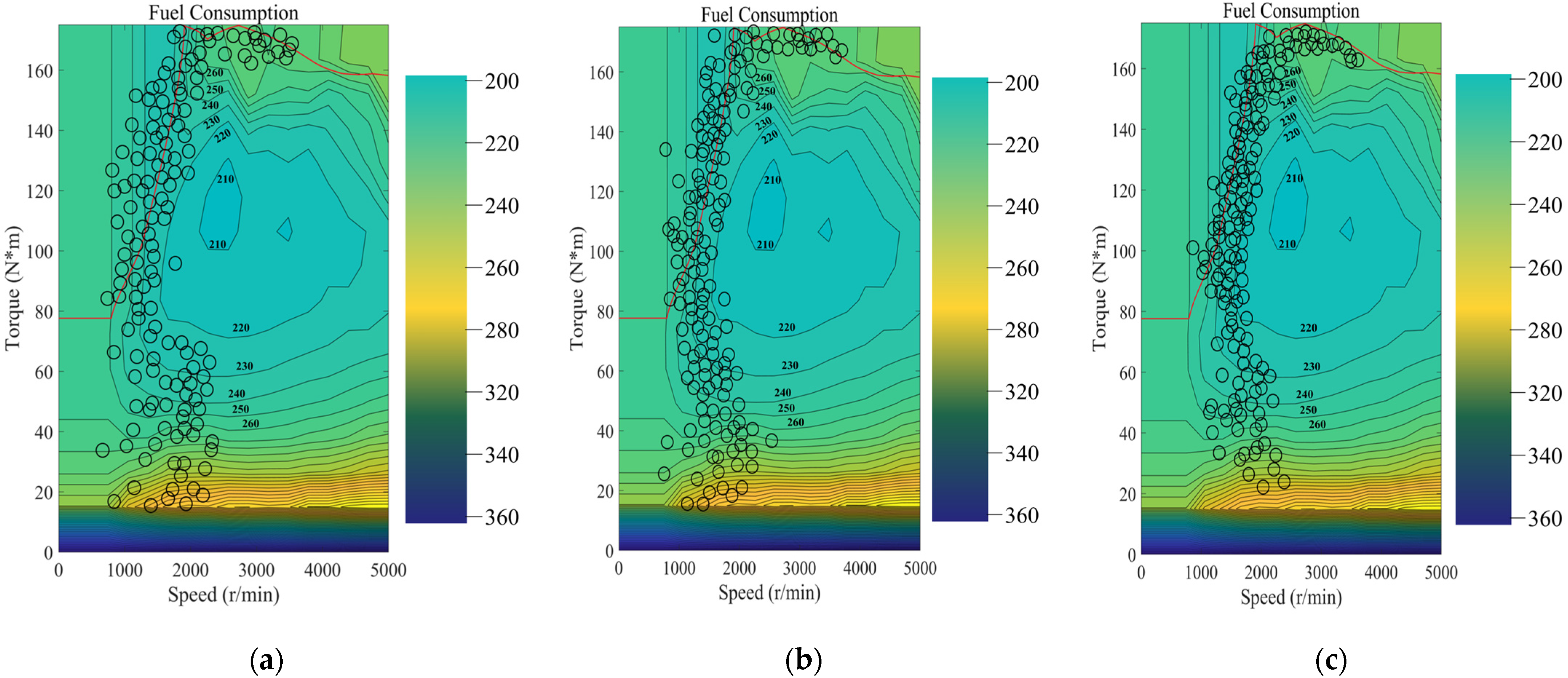
Figure 4 and Figure 5 at the vehicle level compare the battery SOC value curve and the engine operating point for the three algorithms—DQN, DDPG, and ALDE—under the new driving cycle. In Figure 4, the SOC curve of the DQN algorithm and DDPG method fluctuates substantially as the SOC value changes, with the highest fluctuation range reaching roughly 0.4. Due to the presence of the driving condition block memory library, under the control of the ALDE algorithm, the SOC curve exhibits reduced overall fluctuations in the new driving cycle. This indicates that the ALDE agent is capable of promptly responding to completely new dynamic environments and possesses stronger adaptability. In addition, due to the reduced fluctuations in SOC, the lifespan of the battery has also been improved.
Figure 5 presents the universal characteristic map of the engine, where the color bar provides a third dimension of information—fuel consumption rate, measured in grams per kilowatt-hour (g/kWh). The varying shades of color visually represent different levels of fuel consumption. The solid red line represents the empirically derived optimal fuel consumption curve. Its purpose is to reduce time and computational resources wasted by the agent in exploring optimal fuel consumption curve.
In Figure 5, the engine operating points for three algorithms—DQN, DDPG, and ALDE—are illustrated, with the red line representing optimal fuel consumption. The DQN algorithm shows a scattered distribution of points, many of which are above the red line, indicating higher fuel consumption compared to optimal performance, though some points approach the red line. The DDPG algorithm demonstrates a more concentrated distribution, with several points closely aligning with the red line, suggesting better fuel efficiency overall, although some points still exceed optimal consumption. In contrast, the ALDE algorithm exhibits a varied distribution, with several points significantly below the red line, indicating instances of optimal fuel consumption, but it also contains points above the red line. Overall, DDPG appears to perform better in terms of fuel efficiency, while all three algorithms show varying degrees of performance relative to the optimal behavior.
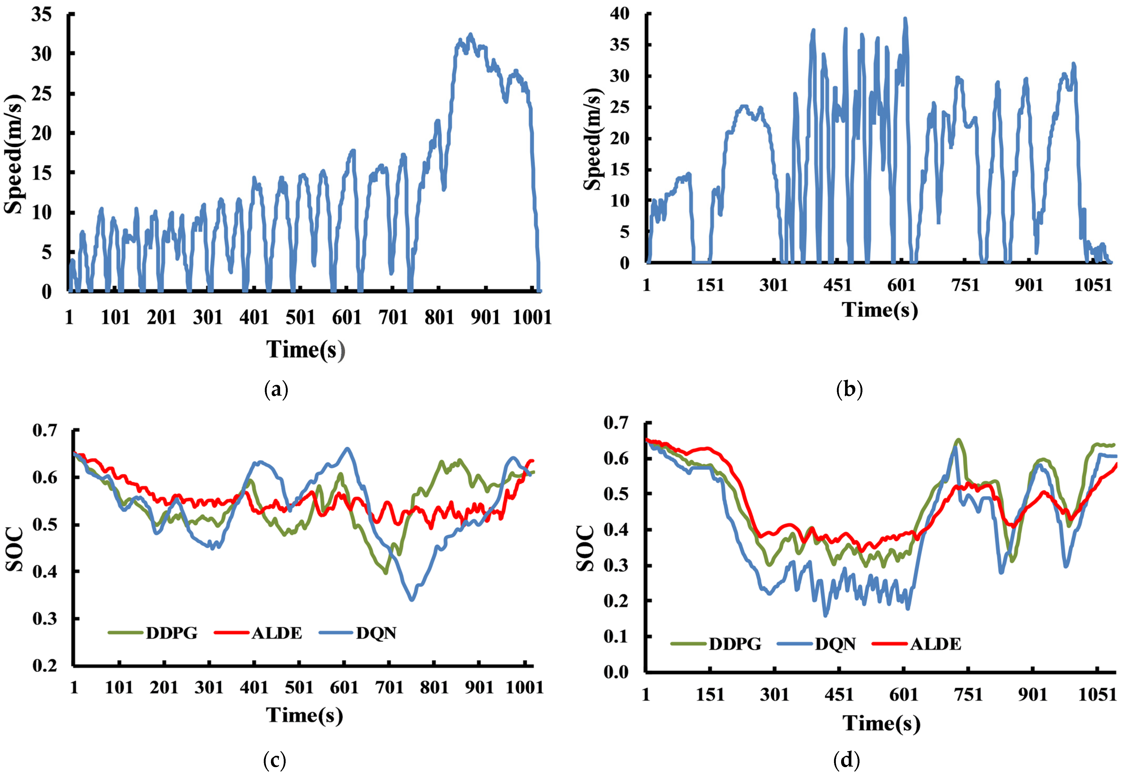
In order to demonstrate the robustness of the ALDE algorithm, we have created two additional completely new driving conditions. These driving conditions are derived from combinations of condition blocks extracted from the DQN and DDPG training sets. The driving conditions are shown in Figure 6a,b, and the corresponding SOC curves are shown in Figure 6c,d. The conclusion remains the same.
The comparison of fuel consumption values under three general driving cycles and one new driving cycle is shown in Table 3. Fuel usage is reduced by roughly 5% compared with the traditional DDPG algorithm, and fuel consumption is decreased by roughly 8% compared with DQN. Therefore, the ALDE algorithm performs well in terms of energy savings and battery SOC value.

4.2. Hardware-in-Loop Experiment

4.2.1. Hardware-in-the-Loop Experimental Platform

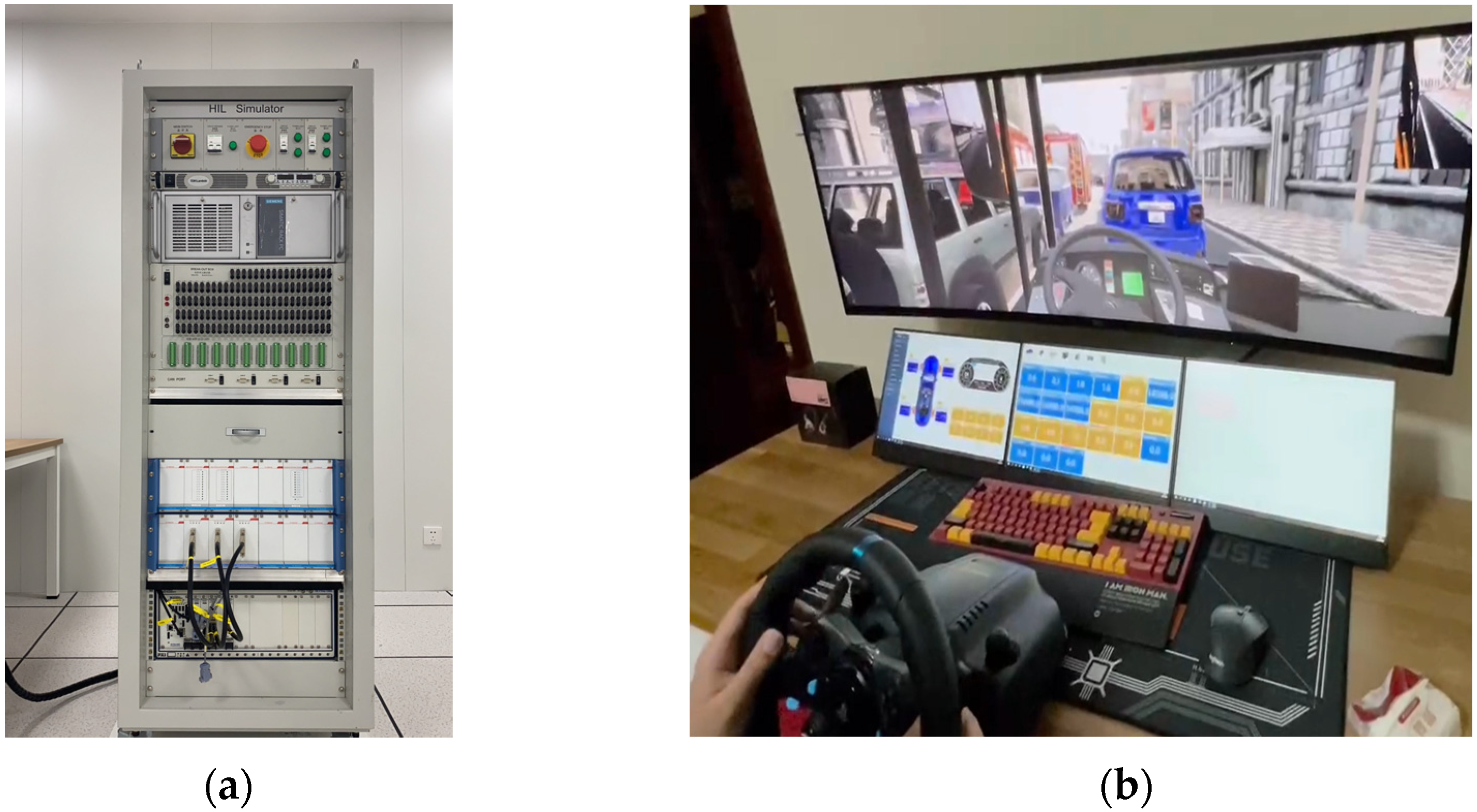
The paper integrates actual vehicle controller hardware and employs dSPACE real-time control simulation equipment to establish an HIL testing platform for experimental research. The HIL testing platform for the vehicle control strategy comprises a host computer, Control Desk control platform, RapidECU_U2 rapid prototype controller, and dSPACE/Simulator real-time simulation system.
In this setup, the dSPACE/Simulator is employed to create a real-time testing environment. The host computer, rapid prototype controller, and simulation system are interconnected via a CAN bus. The host computer manages the downloading of simulation models and driver board interfaces to both the simulator and the rapid prototype controller. The Control Desk platform serves to develop a real-time monitoring interface, facilitating the observation of the simulation process and recording of relevant data. A low-voltage DC power supply and power distribution box provides 24 V DC power to the vehicle controller, while the host computer communicates with the lower computer through a CAN bus module.
The specific implementation process for the hardware-in-the-loop system is as follows: First, resulting from the vehicle simulation structure, the RTI module of the host computer creates a longitudinal simulation model for HIL testing, which is then compiled into a dl1 file and downloaded to the dSPACE/Simulator. Next, using the Codewarrior embedded development environment, we develop embedded control software for the adaptive control strategy. This strategy is compiled into C code using the RTW tool in Matlab/Simulink and programmed into the RapidECU using MeCa V1.5 software via a USBcan downloader.
Finally, the host computer, controller, and simulator are connected through a CAN network to form a local area network, enabling seamless communication among the components. After configuring the simulation monitoring interface on the host computer, we can effectively monitor the vehicle’s operational status and facilitate data reading and storage.

4.2.2. Simulation of Hardware-in-the-Loop Experiment

To assess the potential practical applications of the proposed EMS, HIL experiments were conducted. The integrated systems are depicted in Figure 7a,b [40].
The data detection system, situated below the driver system, is integrated with it. Data interaction is achieved through CAN communication technology allowing for the real-time acquisition of steering wheel angle, acceleration, and brake pedal data. These data are then fed into the vehicle control unit (VCU).
HIL experiments adhere to driving cycles presented in Table 3. Focusing on the new driving cycle, Figure 8a illustrates the HIL results for SOC trajectory (the data sampling frequency is 1000 Hz, and the data undergo filtering processing), and Figure 8b demonstrates the engine operating points. The HIL experiment results in Figure 8a,b are essentially consistent with the simulation tests. Additionally, equivalent fuel consumption for simulated and HIL tests is presented in Table 4. The HIL results demonstrate a high level of agreement with the simulation results, clarifying the fuel-saving performance of the ALDE algorithm.

5. Conclusions and Future Work

We propose a strategy for the vehicle agent that enables it to adaptively handle dynamic environments by modifying its behavior accordingly. We provide a memory library to help the agent make timely adaptive responses to the environment. The learning agent can search the stored repository, find the most similar experience, or extend new experiences to the repository during different periods of time. We combine the Dirichlet and EM algorithms to continuously aggregate and update driving condition clusters. The results indicate that the ALDE strategy efficiently clusters the environment in the potential space, enables memory library utilization, retrieves previously seen environments, and adaptively guides the agent’s actions. The reward curve during training indicates that the ALDE strategy successfully learns from past knowledge, quickly adjusts to changing environments, and converges rapidly. From the perspective of vehicle operation, the engine’s operating point remains near the optimal working curve, resulting in minimal SOC fluctuation.
In our future work, we aim to further explore how to integrate additional relevant factors into the state representation, such as road gradient, traffic conditions, and driver behavior. By including these elements, we hope to gain a more comprehensive understanding of the interactions among state variables, which will enhance the model’s decision-making capabilities and generalization. In addition, we also recognize that computational burden is a crucial consideration in assessing the feasibility of algorithms, and we will continue to prioritize this aspect in our future research.

Author Contributions

Conceptualization, S.S. and C.Z.; methodology, S.S.; software, C.Z.; validation, C.Q., C.S. and S.S.; formal analysis, F.X.; investigation, L.J.; resources, F.T.; data curation, S.S. and C.Z.; writing—original draft preparation, C.Z.; writing—review and editing, S.S.; visualization, S.S. and C.Z., C.Q.; supervision, S.S.; project administration, S.S.; funding acquisition, C.Q. All authors have read and agreed to the published version of the manuscript.

Funding

The Project supported by the Science Fund of State Key Laboratory of Advanced Design and Manufacturing Technology for Vehicle No.82315002.

Data Availability Statement

Data is contained within the article.

Acknowledgments

The Project supported by the Science Fund of State Key Laboratory of Advanced Design and Manufacturing Technology for Vehicle No.82315002. Any opinion expressed here solely belongs to the authors and does not represent that of the sponsors. The authors thank the experienced anonymous reviewers for their constructive, valuable suggestions that improve the overall quality of this paper.

Conflicts of Interest

The authors declare that they have no conflicts of interest to disclose in relation to this research. Specifically, none of the authors have any financial, personal, or professional relationships that could potentially bias the results or interpretation of the data presented in this paper. Additionally, no external funding was received for this study, eliminating any potential for funder-related biases. The authors maintain the highest standards of integrity and objectivity in conducting and reporting this research.

References

  1. Talari, K.; Jatrothu, V.N. A Review on Hybrid Electrical Vehicles. Stroj. Cas. J. Mech. Eng. 2022, 72, 131–138. [Google Scholar] [CrossRef]
  2. Gaidar, S.; Karelina, M.; Laguzin, A.; Quang, H.D. Impact of operational factors on environmental safety of internal combustion engines. Transp. Res. Procedia 2020, 50, 136–144. [Google Scholar] [CrossRef]
  3. Yu, X.; Zhu, L.; Wang, Y.; Filev, D.; Yao, X. Internal combustion engine calibration using optimization algorithms. Appl. Energy 2022, 305, 117894. [Google Scholar] [CrossRef]
  4. Allwyn, R.G.; Al-Hinai, A.; Margaret, V. A comprehensive review on energy management strategy of microgrids. Energy Rep. 2023, 9, 5565–5591. [Google Scholar] [CrossRef]
  5. Bagwe, R.M.; Byerly, A.; Dos Santos, E.C., Jr.; Ben-Miled, Z. Adaptive Rule-Based Energy Management Strategy for a Parallel HEV. Energies 2019, 12, 4472. [Google Scholar] [CrossRef]
  6. Wang, Y.; Li, W.; Liu, Z.; Li, L. An Energy Management Strategy for Hybrid Energy Storage System Based on Reinforcement Learning. World Electr. Veh. J. 2023, 14, 57. [Google Scholar] [CrossRef]
  7. Inuzuka, S.; Zhang, B.; Shen, T. Real-Time HEV Energy Management Strategy Considering Road Congestion Based on Deep Reinforcement Learning. Energies 2021, 14, 5270. [Google Scholar] [CrossRef]
  8. Huang, K.D.; Nguyen, M.K.; Chen, P.T. A Rule-Based Control Strategy of Driver Demand to Enhance Energy Efficiency of Hybrid Electric Vehicles. Appl. Sci. 2022, 12, 8507. [Google Scholar] [CrossRef]
  9. Fu, X.; Wang, B.; Yang, J.; Liu, S.; Gao, H.; He, B.Q.; Zhao, H. A Rule-Based Energy Management Strategy for a Light-Duty Commercial P2 Hybrid Electric Vehicle Optimized by Dynamic Programming. In Proceedings of the SAE 2021 WCX Digital Summit, Virtual, 13–15 April 2021. [Google Scholar]
  10. Peng, J.; Fan, H.; He, H.; Pan, D. A Rule-Based Energy Management Strategy for a Plug-in Hybrid School Bus Based on a Controller Area Network Bus. Energies 2015, 8, 5122–5142. [Google Scholar] [CrossRef]
  11. Zhou, S.; Chen, Z.; Huang, D.; Lin, T. Model Prediction and Rule Based Energy Management Strategy for a Plug-in Hybrid Electric Vehicle with Hybrid Energy Storage System. IEEE Trans. Power Electron. 2021, 36, 5926–5940. [Google Scholar] [CrossRef]
  12. Peng, J.; He, H.; Xiong, R. Rule based energy management strategy for a series–parallel plug-in hybrid electric bus optimized by dynamic programming. Appl. Energy 2017, 185, 1633. [Google Scholar] [CrossRef]
  13. Ding, N.; Prasad, K.; Lie, T.T. Design of a hybrid energy management system using designed rule-based control strategy and genetic algorithm for the series—parallel plug—in hybrid electric vehicle. Int. J. Energy Res. 2021, 45, 1627–1644. [Google Scholar] [CrossRef]
  14. Guercioni, G.R.; Galvagno, E.; Tota, A.; Vigliani, A. Adaptive Equivalent Consumption Minimization Strategy with Rule-Based Gear Selection for the Energy Management of Hybrid Electric Vehicles Equipped with Dual Clutch Transmissions. IEEE Access 2020, 8, 190017–190038. [Google Scholar] [CrossRef]
  15. Mansour, C.J. Trip-based optimization methodology for a rule-based energy management strategy using a global optimization routine: The case of the Prius plug-in hybrid electric vehicle. Proc. Inst. Mech. Eng. Part D J. Automob. Eng. 2016, 230, 1529–1545. [Google Scholar] [CrossRef]
  16. Chen, Z.; Xiong, R.; Cao, J. Particle swarm optimization-based optimal power management of plug-in hybrid electric vehicles considering uncertain driving conditions. Energy 2016, 96, 197–208. [Google Scholar] [CrossRef]
  17. Lian, R.; Peng, J.; Wu, Y.; Tan, H.; Zhang, H. Rule-interposing deep reinforcement learning based energy management strategy for power-split hybrid electric vehicle. Energy 2020, 197, 117297. [Google Scholar] [CrossRef]
  18. Zhou, Y.; Ravey, A.; Pera, M.-C. A survey on driving prediction techniques for predictive energy management of plug-in hybrid electric vehicles. J. Power Sources 2019, 412, 480–495. [Google Scholar] [CrossRef]
  19. Xu, B.; Rathod, D.; Zhang, D.; Yebi, A. Parametric study on reinforcement learning optimized energy management strategy for a hybrid electric vehicle. Appl. Energy 2020, 259, 114200. [Google Scholar] [CrossRef]
  20. Chaoui, H.; Gualous, H.; Boulon, L.; Kelouwani, S. Deep Reinforcement Learning Energy Management System for Multiple Battery Based Electric Vehicles. In Proceedings of the IEEE Vehicle Power and Propulsion Conference, Chicago, IL, USA, 27–30 August 2018. [Google Scholar]
  21. Aljohani, T.M.; Ebrahim, A.; Mohammed, O. Real-Time metadata-driven routing optimization for electric vehicle energy consumption minimization using deep reinforcement learning and Markov chain model. Electr. Power Syst. Res. 2021, 192, 106962. [Google Scholar] [CrossRef]
  22. Zou, Y.; Liu, T.; Liu, D.; Sun, F. Reinforcement learning-based real-time energy management for a hybrid tracked vehicle. Appl. Energy 2016, 171, 372–382. [Google Scholar] [CrossRef]
  23. Xiong, R.; Cao, J.; Yu, Q. Reinforcement learning-based real-time power management for hybrid energy storage system in the plug-in hybrid electric vehicle. Appl. Energy 2018, 211, 538–548. [Google Scholar] [CrossRef]
  24. Qi, C.; Zhu, Y.; Song, C.; Yan, G.; Xiao, F.; Da, W.; Zhang, X.; Cao, J.; Song, S. Hierarchical reinforcement learning based energy management strategy for hybrid electric vehicle. Energy 2022, 238, 121703. [Google Scholar] [CrossRef]
  25. Lee, H.; Song, C.; Kim, N.; Cha, S.-W. Comparative Analysis of Energy Management Strategies for HEV: Dynamic Programming and Reinforcement Learning. IEEE Access 2020, 8, 67112–67123. [Google Scholar] [CrossRef]
  26. Aljohani, T.M.; Mohammed, O. A Real-Time Energy Consumption Minimization Framework for Electric Vehicles Routing Optimization Based on SARSA Reinforcement Learning. Vehicles 2022, 4, 1176–1194. [Google Scholar] [CrossRef]
  27. Sun, W.; Zou, Y.; Zhang, X.; Gua, N.; Zhang, B.; Du, G. High robustness energy management strategy of hybrid electric vehicle based on improved soft actor-critic deep reinforcement learning. Energy 2022, 258, 124806. [Google Scholar] [CrossRef]
  28. Guo, L.; Liu, H.; Han, L.; Yang, N.; Liu, R.; Xiang, C. Predictive energy management strategy of dual-mode hybrid electric vehicles combining dynamic coordination control and simultaneous power distribution. Energy 2023, 263, 125598. [Google Scholar] [CrossRef]
  29. Liu, Y.; Zhang, Y.; Yu, H.; Nie, Z.; Liu, Y.; Chen, Z. A novel data-driven controller for plug-in hybrid electric vehicles with improved adaptabilities to driving environment. J. Clean. Prod. 2022, 334, 130250. [Google Scholar] [CrossRef]
  30. Akamine, K.; Imamura, T.; Terashima, K. Gain-scheduled control for the efficient operation of a power train in a parallel hybrid electric vehicle according to driving environment. Nippon. Kikai Gakkai Ronbunshu C Hen Trans. Jpn. Soc. Mech. Eng. Part C 2003, 69, 1648–1655. [Google Scholar] [CrossRef]
  31. Chen, J.; Qian, L.; Xuan, L.; Chen, C. Hierarchical eco-driving control strategy for hybrid electric vehicle platoon at signalized intersections under partially connected and automated vehicle environment. IET Intell. Transp. Syst. 2023, 17, 1312–1330. [Google Scholar] [CrossRef]
  32. Zhang, Z.; Liu, H.; Lei, M.; Yan, X. Review on the impacts of cooperative automated driving on transportation and environment. Transp. Res. Part D Transp. Environ. 2023, 115, 103607. [Google Scholar] [CrossRef]
  33. Zhu, J.; Wei, Y.; Kang, Y.; Jiang, X.; Dullerud, G.E. Adaptive deep reinforcement learning for non-stationary environments. Sci. China Inf. Sci. 2022, 65, 225–241. [Google Scholar] [CrossRef]
  34. Wang, H.; Liu, N.; Zhang, Y.; Feng, D.; Huang, F.; Li, D.; Zhang, Y. Deep reinforcement learning: A survey. Front. Inf. Technol. Electron. Eng. 2020, 21, 1726–1744. [Google Scholar] [CrossRef]
  35. Ha, J.; An, B.; Kim, S. Reinforcement Learning Heuristic A. IEEE T. Ind. Inform. 2023, 19, 2307–2316. [Google Scholar] [CrossRef]
  36. Zhu, Z.; Lin, K.; Jain, A.K.; Zhou, J. Transfer Learning in Deep Reinforcement Learning: A Survey. IEEE Trans. Pattern. Anal. Mach. Intell. 2023, 45, 13344–13362. [Google Scholar] [CrossRef]
  37. Lv, H.; Qi, C.; Song, C.; Song, S.; Zhang, R.; Xiao, F. Energy management of hybrid electric vehicles based on inverse reinforcement learning. Energy Rep. 2022, 8, 5215–5224. [Google Scholar] [CrossRef]
  38. Balooch, A.; Wu, Z. A new formalization of Dirichlet-type spaces. J. Math. Anal. Appl. 2023, 1, 127322. [Google Scholar] [CrossRef]
  39. Gaisin, A.M.; Gaisina, G.A. On the Stability of the Maximum Term of the Dirichlet Series. Russ. Math. 2023, 67, 20–29. [Google Scholar] [CrossRef]
  40. Qi, C.; Wang, D.; Song, C.; Xiao, F.; Jin, L.; Song, S. Action Advising and Energy Management Strategy Optimization of Hybrid Electric Vehicle Agent Based on Uncertainty Analysis. IEEE Trans. Transp. Electrif. 2024, 10, 6940–6949. [Google Scholar] [CrossRef]
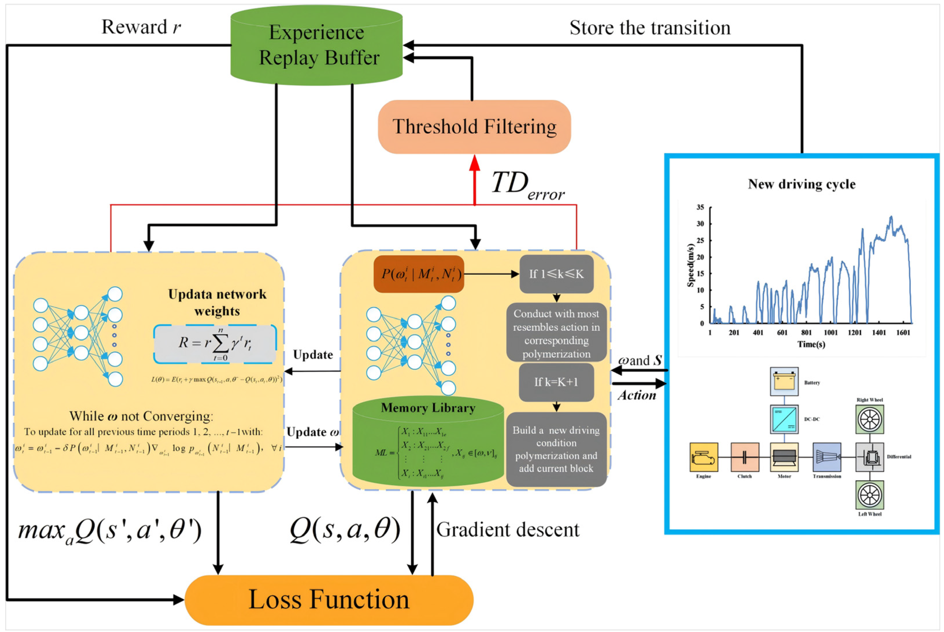
Figure 1. Flow chart of ALDE algorithm.
Designs 08 00102 g001
Figure 2. Definition of driving condition block.
Designs 08 00102 g002
Figure 3. (a) New driving cycle diagram; (b) driving cycle cluster; (c) reward value change curve.
Designs 08 00102 g003
Figure 4. SOC value change curve. The blue and green lines represent the DQN and DDPG algorithms, respectively. The red line represents the ALDE algorithm.
Designs 08 00102 g004
Figure 5. Engine operating points. (a) DQN; (b) DDPG; (c) ALDE.
Designs 08 00102 g005
Figure 6. New driving cycles and SOC curve: (a) cycle 2; (b) cycle 3; (c) SOC curve of new driving cycle 2; (d) SOC curve of new driving cycle 3.
Designs 08 00102 g006
Figure 7. Integrated system and driver operating system: (a) integrated system; (b) integrated system.
Designs 08 00102 g007
Figure 8. SOC variation values and engine operating points: (a) integrated system; (b) driver operating system.
Designs 08 00102 g008
Table 1. Other parameters of the vehicle.
SymbolParameterValues
EngineMaximum power92 kW
Maximum torque175 Nm
Maximum speed6500 rpm
Traction motorMaximum power30 kW
Maximum torque200 Nm
Maximum speed6000 rpm
BatteryCapacity5.3 Ah
Voltage266.5 V
Table 2. Specific contribution rate and cumulative contribution rate.
IngredientContribution Rate/%Cumulative Contribution Rate/%
Average Speed 45.1345.13
Idle Time23.2868.41
Distance10.4778.88
Table 3. Fuel consumption.
AlgorithmDDPGDQNALDEFuel Consumption Reduction Rate Compared with DDPGFuel Consumption Reduction Rate Compared with DQN
Driving
Cycles
WLTP6.74 L/100 km7.05 L/100 km6.32 L/100 km6.23%10.35%
US066.16 L/100 km6.47 L/100 km5.85 L/100 km5.03%9.58%
LA926.44 L/100 km6.68 L/100 km6.08 L/100 km5.60%8.98%
New
driving cycle
7.38 L/100 km7.87 L/100 km7.13 L/100 km3.39%9.04%
Table 4. Fuel consumption (HIL).
AlgorithmALDE/SIMALDE/HIL
Driving Cycles
WLTP6.32 L/100 km6.29 L/100 km
US065.85 L/100 km5.91 L/100 km
LA926.08 L/100 km6.11 L/100 km
New
driving cycle
7.13 L/100 km7.07 L/100 km
Disclaimer/Publisher’s Note: The statements, opinions and data contained in all publications are solely those of the individual author(s) and contributor(s) and not of MDPI and/or the editor(s). MDPI and/or the editor(s) disclaim responsibility for any injury to people or property resulting from any ideas, methods, instructions or products referred to in the content.