Abstract
Saving energy and resources has become increasingly important for industrial applications. Foremost, this requires knowledge about the energy requirement. For this purpose, this paper presents a state-based energy requirement model for mobile robots, e.g., automated guided vehicles or autonomous mobile robots, that determines the energy requirement by integrating the linearized power requirement parameters within each system state of the vehicle. The model and their respective system states were verified using a qualitative process analysis of 25 mobile robots from different manufacturers and validated by comparing simulated data with experimental data. For this purpose, power consumption measurements over 461 operating hours were performed in experiments with two different industrial mobile robots. System components of a mobile robot, which require energy, were classified and their power consumptions were measured individually. The parameters in the study consist of vehicle speed, load-handling duration, load, utilization, material flow and layout data, and charging infrastructure system frequency, yet these varied throughout the experiments. Validation of the model through real experiments shows that, in a confidence interval, the relative deviation in the modeled power requirement for a small-scale vehicle is , whereas, for a mid-scale vehicle, it is . This sets a benchmark for modeling the energy requirement of mobile robots with multiple influencing factors, allowing for an accurate estimation of the energy requirement of mobile robots.
1. Introduction
At a time when the validity of the European Union’s Energy Efficiency Directive [1] is approaching and sustainability and resource efficiency have become major concerns, innovative solutions for reducing energy requirements are needed. In the field of intralogistics, the use of battery powered mobile robots, such as automated guided vehicles (AGVs) or autonomous mobile robots (AMRs) for material flow, has been on the rise for years. AGVs can perform their tasks in a time-efficient manner but could also save energy and reduce the environmental impact through smaller energy storage systems (ESSs). Available ESSs for AGVs are currently designed for continuous operating times of 8 h to 16 h. Some manufacturers even advertise their energy storage capacity for operation times up to 48 h. To determine the actual energy storage capacity required in operation, it is necessary to obtain knowledge of the energy requirement of AGVs under various influencing factors. Despite the increasing prevalence of mobile robots in industrial applications, there is a lack of a comprehensive model to accurately estimate their energy requirement under multiple constraints. In the scientific literature, some approaches for modeling energy requirements can be found, but they only consider single system components, such as drives, controls, or load-handling devices (LHDs). In an extensive review of existing literature in this field, it is notable that no comprehensive model has been found.
This paper presents a comprehensive state-based energy requirement model (ERM) that takes into account various influencing factors on the energy requirement of AGVs. This model can be used for different vehicle types and various transport layouts. A validation was performed by 15 real experiments using two different vehicles. In these, parameters of transport layout, transport orders, utilization, speed, charging system distribution, load-handling time, charging strategy, and operating time were varied. Furthermore, a discrete time simulation model was developed in Java that can be used to simulate real experiments. In addition to the ERM, a simulation model consists of functional modules such as a dispatcher, which distributes transport orders to the AGV being simulated. The energy requirement can be calculated during simulation by integrating power requirement parameters over time. A qualitative analysis of system processes of 25 different AGVs allowed the ERM and their states to be verified. Then, the model was validated by comparing the simulative and experimental data. The results of the validation show that the ERM is suitable for a comprehensive approximation of the energy requirement of AGVs under multiple constraints.
In Section 2, an overview of the most important work in the field of power and energy requirement modeling of AGVs is presented. Furthermore, methods concerning operating and charging strategies, dispatching, ESS modeling, and material flow system modeling are described. In Section 3, the ERM and the energy requirement approximation are presented. Its implementation through a simulation model is described in Section 4. The experimental design, the description of the experimental environment, and the methods for verification and validation are described in Section 5. In Section 6, the quantitative results of the validation, as well as further findings, are presented, followed by a conclusion of the entire study.
2. Related Work
This section overviews related work in the area of modeling power and energy requirements for mobile robots such as AGVs or AMRs and operation and charging strategies, as well as dispatching algorithms. Furthermore, this section includes technical fundamentals of energy storage systems that were used most in the investigation of this paper. Finally, a further investigated model for describing material flow and layout configurations is presented.
2.1. Power and Energy Requirement Modeling of AGVs
The energy or power requirement of components of mobile robots was investigated in several studies, which are considered in this section. At the level of factory and logistics planning, Freis and Günthner [2] presented an analytical model for determining the overall energy efficiency of logistics centers. In this context, key figures for industrial trucks were considered for the intralogistics submodel for energy requirement determination. Key figures include the number of vehicles, the average electrical power consumption per hour, the operating hours per year, and the battery charging efficiency. Furthermore, Mueller et al. [3] presented an approach for energy-efficiency-oriented planning of logistics systems by theoretical aspects using an AGV as an example.
At the level of logistic planning, Ebben [4] investigated the impact of battery constraints on AGVs on logistics performance. The results of his work show that automated contact-based charging processes lead to better logistics performance compared to battery swapping. At the control system level (cf. [5]), Mei et al. [6] presented a power requirement model for an AGV. By varying velocity under energy and travel time constraints, a minimization of the total travel time and energy requirement compared to two heuristics could be achieved. At the same level, Qiu et al. [7] have presented an energy consumption minimization method for the route planning of heterogeneous AGV fleets. Experiments showed that energy consumption could be reduced by at least 6.08% compared to methods for minimizing transportation distances.
Kim and Kim [8] presented a minimum energy translational trajectory planning algorithm for a differential-driven mobile robot and adapted it to a three-wheel-driven mobile robot in a subsequent study [9]. Simulation experiments reveal at least energy savings for differential-driven mobile robots and energy savings for three-wheel-driven mobile robots. Another model for minimizing energy requirements for differential-driven AGVs is shown by Liu and Sun [10] in their paper. Smooth trajectories are obtained by optimization, where the velocity is varied to minimize energy requirements. Related work was completed by Kabir and Suzuki [11], where different routing heuristics were studied considering energy requirements.
Stampa et al. [12] have presented a mathematical model for the estimation of the energy consumption of an omnidirectional AGV, which can be used to investigate different trajectories between the same points for their energy consumption. Comparison with data from real experiments has shown that the energy consumption data from the model are coherent with the measurements.
Hou et al. [13] have presented a model that can be used to determine the power requirement of drives and control during the standby, acceleration, and stable states. Real experiments performed to determine the energy requirement were further investigated by Niestroj et al. [14]. They present an energy requirement model for an AGV using a hybrid ESS consisting of Li-ion and hydrogen. For the simulative experiments, the average energy consumption of an AGV under selected operating conditions was measured at the beginning and subsequently investigated by varying the speed and load. This model, as well as the model by Stampa et al. [12] and Hou et al. [13], does not consider transport orders or transport distances.
The most related works on modeling power and energy requirements of AGVs are [15,16]. Hamdy [15] presents a simulation model to determine the optimal number of vehicles considering energy constraints. The state-based simulation model features the states blocking, traveling empty, traveling loaded, accelerating empty, accelerating loaded, decelerating empty, decelerating loaded, picking, and dropping, whereby each has constant total power. The interpreted relations of the states are shown in the following Figure 1 as a state diagram.
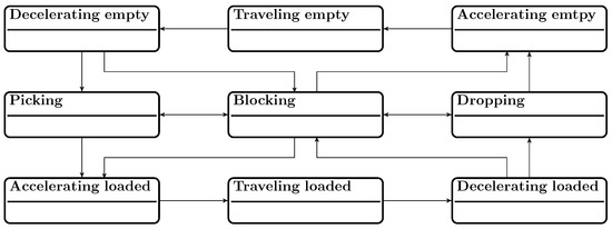
Figure 1.
State-based activity model for AGVs. Own illustration, based on [11,15,17].
Finally, the work of Meissner and Massalski [16] is mentioned, in which the electrical power of the drives of an AGV with differential drives was measured and analyzed for the procedure. In a state-based simulation model, the states accelerating, driving, and decelerating were represented and reported a relative average deviation in the energy requirements of the drives as . Furthermore, the load-handling process was investigated in detail. In experiments, the driving speed and the transported load were varied. Through performance measurements of the LHD and data analysis, five active sub-states could be identified. These are the acceleration of the LHD, lifting without load, lifting load absorption (where the lifting load increases), lifting under full load, and breaking, which are shown in the following Figure 2 as a state diagram.
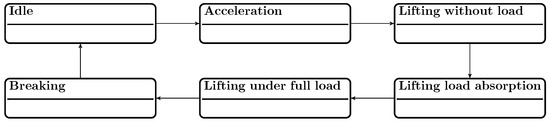
Figure 2.
State-based activity model for an LHD of an AGV. Own illustration, based on [16].
The relative deviation in the energy consumption modeling of the load-handling device was stated as . The findings on energy consumption were processed quantitatively and show that the power does not vary linearly with increasing speed and transport weight. The correlation resulting from the investigations can be further transferred into a nonlinear optimization problem in order to determine an optimum operating point with minimum energy consumption. In Table 1, the previously mentioned studies on the power and energy requirement modeling of AGVs are classified according to relevant characteristics, which will be explained in more detail later in this paper. Compared to the related studies, the energy requirement model (ERM) described in this paper is classified in the bottom row of Table 1.

Table 1.
Literature review on modeling power and energy requirement of AGVs. Charging strategies: C = capacitive, I = interim, O = opportunity. : total vehicle power. (•): Considered. (-): Not considered.
It can be seen that scientific studies with real experiments have neglected the characteristics of operating states, charging strategy, layout and material flow, utilization, and CIS distribution, whereas simulation-based studies without real experiments focus on the variation in material flow and layout. Furthermore, it is clear that the modeling of load-handling power and energy requirement was only investigated by [16]. The ERM was simulated and further validated by real experiments, where the vehicle components were examined individually based on state. Compared to the corresponding models, all other properties of Table 1 are fully covered. Variables marked with tot indicate the total energy or power of the vehicle without separating individual components. Drives and controls were only considered separately by [6], whereas constant values for the power and energy requirements of the controls were assumed in other studies. If specific charging strategies were applied, they are named C for capacitive and O for opportunity. The charging strategies are described in more detail in the following section.
2.2. Operating and Charging Strategies
A charging strategy describes the charging process of each individual vehicle at the control system level according to [5,23]. Operating strategies with energy constraints are to be distinguished from charging strategies because they describe strategies on the process control level according to [5,23], where the charging states of the vehicles and the utilization rates of the charging systems impact the behavior regulation of the AGVs. Jodejko-Pietruczuk and Werbińska-Wojciechowska [22] presented a multi AGV simulation model for this purpose, where the state of charge (SoC) of the ESS is taken into account. For their studies, the number of charging systems in the layout was varied. Colling et al. [20] have presented a method where the SoC of vehicles are distributed in a cycle-oriented manner to maximize the utilization of charging stations and balance the overall system availability. Further work on operating strategies was performed by Singh et al. [18] and Abderrahim et al. [19], where each presented and studied a scheduling model with battery constraints. In a previous paper, a review of charging and operating strategies with energy constraints for AGV systems was conducted [24]. The three most common charging strategies are the capacitive operation (capacitive), the capacitive operation with intermediate charging (interim), and the opportunity charging (opportunity) [24,25,26], which were already mentioned in Table 1. Since only individual vehicles are considered in this paper, the operation strategies with energy constraints from [24] are not relevant. However, dispatching algorithms, which run on the supervision level, are of relevance.
2.3. Dispatching
Dispatching or task allocation describes the systematic distribution of transport orders to the vehicles of a transport system. Whereas, in centralized allocation, a fleet manager has information about the utilization of the vehicles and distributes the orders strategically, in decentralized allocation, the orders are negotiated between the vehicles and distributed [27].
Various methods from the literature for dispatching were summarized by [28,29]. The methods described aim to optimize task allocation according to at least one criterion. Typical optimization criteria are the minimization of the number of required AGVs, the minimization of the sum of distances to be driven, the minimization of buffer sizes at the stations (both input and output), the minimization of the waiting time of a transport order, the minimization of possible blockages due to backlogs, and the maximization of the production ratio. In addition to single-objective optimization, Zamiri Marvizadeh and Choobineh [30] presented a dispatching method in which both input and output queues of stations are balanced.
2.4. Modeling Energy Storage Systems (ESSs)
Many scientific studies modeled ESSs in order to use them to acquire knowledge regarding their behavior toward influencing factors such as calendrical and cyclic aging, temperature, charging power, and others (cf. [31,32,33,34,35,36,37,38,39,40]). Usually only an impact on the maximum capacity of ESSs was investigated. Since this paper is about modeling the power and energy requirement of AGVs under certain constraints, only a linear relation is assumed in determining the current capacity and SoC, respectively. In AGV systems, lead–acid ESSs are still widely used. Even the latest guideline VDI 2510 part 4 [25] still includes parameters for the design of lead–acid ESSs for AGVs. The most typical ESSs are lithium cobalt oxide (LCO), although other types of lithium-based ESSs are frequently used in AGVs due to their low specific energy density. The characteristics (cf. Table A6) show that the cell voltages and the C-rates, as well as the maximum voltage strokes, vary strongly for the ESS. Another type of energy storage is the electronic double-layer capacitor (EDLC). This term describes capacitors with extended capacity compared to electrolytic capacitors. Unlike electrochemical ESSs, the electrical energy is stored by an electric field. An EDLC has a capacitance of to over at typically to per cell [24].
2.5. Material Flow System Description
The literature presented in Section 2.1 partially considers material flow and layout data in its investigations, where transport distances are a major influencing factor for energy requirements (cf. [7,15,18,21]). In a previous paper [41], an approach to modeling material flow systems was presented. The model of a material flow system is called material flow and layout composition and consists of transport orders and the distance relationships between stations. The transport orders and distance relationships are modeled in the form of matrices (cf. [41]), whereas describes the transport matrix of a composition and the distance matrix. Furthermore, a taxonomy of these material flow models was presented. The taxonomy allows for classification compositions in flow path orientation, layout topology, and task structure.
3. Energy Modeling
In order to model an energy requirement of AGVs, components of an AGV that have an energy requirement must be defined first. In the next step, the power requirement of the respective system components was defined as a function of its influencing factors. Finally, the total energy requirement can be determined by summing up the power requirements of the respective system components over time.
3.1. System Components
The individual components vary depending on the AGV type. For this study, three main components—drives, controls, and the load-handling device (LHD)—were identified and defined (cf. Figure 3).
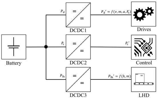
Figure 3.
Block diagram of defined AGV power requirement components.
Drives include the electrical power of the drives and motor controls as a function of velocity, acceleration, and the weight of the load being transported. All remaining parameters, such as slip, expressed as friction force, are considered in the linear power requirement approximation. Motor controllers or regulators are also part of this power requirement component. Controls include all components that are responsible for control, communication, navigation, and localization, as well as system safety. This includes, for example, lighting equipment, safety controls, and safety sensors. Here, unlike that shown in Figure 3, controls can consist of several individual control units (cf. [24,42]). Finally, the LHD includes all components that are involved in the load-handling process. These include lifting or transfer drives and hydraulic pumps, as well as associated control, communication, and sensor units. As shown in Figure 3, for each power requirement component, DC-DC converters (DCDCs) are connected in series to regulate the voltage level between an energy storage system and the system components. The efficiency of the DCDCs is typically described as a function of the output current [43]. Therefore, the power requirement of the system components considering DCDCs is related to the actual power requirement of the components as follows:
3.2. Process Analysis
To be able to describe the behavior of different AGVs in a holistic way, process states have to be identified. In addition to the two state diagrams presented for AGV process description (cf. Figure 1 and Figure 2), Komma et al. [44] and Flake [45] have presented further state diagrams to model system behaviors of AGVs. From these previous studies, the process states of acceleration without load, acceleration with load, drive without load, drive with load, deceleration with load, deceleration without load, pickup, deliver, and standby can be derived. Standby summarizes the processes of waiting, blocking, and idle. In the course of a qualitative process analysis, in which 25 different AGVs were examined, it was found that, in addition to previously identified states, four additional states are required in order to develop a holistic description model. These are Prepare docking, Dock, undock, and Prepare driving. Prepare docking includes waiting times for process calculation and initialization of the LHD for Dock. Similarly, Prepare driving includes process calculation waiting times and initialization of the LHD for driving. The initialization for driving includes substates that bring the vehicle into a state ready for driving. These include, for example, lowering the LHD to a defined transport height.
3.3. Impact Analysis
After defining the power requirement components and process states for AGVs, the factors that impact the power requirements of these system components were identified. The literature review presented in Section 2.1 shows that speed, acceleration, weight of the load, and movement direction have a significant impact on the electrical power requirement of the drives. Another impact on the power requirement of the controls is ambient temperature. Cebrian and Natvig [46] stated that the power requirement of processors is highly temperature dependent. Finally, the weight of the load has a significant impact on the power requirement of the LHD (cf. Table 1, [16]). Eggers et al. [47] analyzed the impact of temperature on the power requirement of industrial robots. They found that increasing temperature reduces the friction force in the joints and thus decreases the total power requirement. The same could apply for LHDs of AGVs but this is not considered further in this work.
Table 1 shows that the energy requirement E is often modeled as a function of time t or as a function of transport distance d. The transport time t or the transport distances d are further impacted by other characteristics as mentioned in Table 1. These include material flow and layout, operating strategy, dispatching method used, and CIS distribution. Based on the findings of this impact analysis, a model for approximating the energy requirement was developed, described in more detail in Section 3.5 and Section 3.6.
3.4. Linear Power Approximation
To model the power requirement of the drives, the functional relations between mass, velocity, acceleration, deceleration, and the movement direction are simplified by linear approximation. This approach was also used in [2,11,15,17,18,19,20,48]. The power requirements of the individual system components are assigned to different states, which are listed in Table 2.
Table 2.
ERM mean power parameter for different operation states.
They are mapped to the states of the ERM (cf. Section 3.5). In addition to the parameters listed above, further parameters are required for the ERM. These are acceleration , deceleration , maximum velocity , C-rate for charge, and typical process state times as well as material flow and layout composition (cf. Section 2.5).
3.5. Energy Requirement Model (ERM)
Based on the identification of the system components with a power requirement (cf. Section 3.1), a process analysis (cf. Section 3.2), a power requirement impact analysis (cf. Section 3.3), a resulting linear power requirement approximation (cf. Section 3.4), and a holistic state-based model were elaborated as shown in Figure 4. Therefore, the ERM can approximate the power requirement of different AGVs.
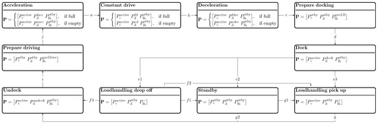
Figure 4.
State-based ERM of an AGV.
Figure 4 shows 10 different states describing the previously mentioned process states of an AGV, each containing a vector , including the individual mean power requirements:
The arrows connecting the states describe the possible linkage of states to an overall process. The initial state is standby. After standby, either a run can be started via states Undock (g2), Prepare driving (i), and Acceleration (j), or a load can be picked up at the current position (Loadhandling pick up via g1). If the vehicle is in Acceleration state, then state Constant drive is achieved after reaching the target velocity (a). With the initiation of a braking process at the end of a run, Deceleration (b) becomes active. After stopping, the next states Prepare docking and Dock become active in sequence. After reaching standstill again, three states are possible: Loadhandling pick up via (e3), Loadhandling drop off via (e1), or Standby via (e2). Standby can be reached if waiting times are required due to interruptions in the operating flow. If the AGV is in Loadhandling drop off state, Standby (f1), Loadhandling pick up (f2), or Undock (f3) state is reachable accordingly. From Standby state, either Undock (g2) can be initiated directly or a load can be picked up (Loadhandling pick up via g1).
3.6. Total Energy Requirement Approximation
As a result of the impact analysis (cf. Section 3.3), the distance is not sufficient for the approximation of the total energy requirement of AGVs. To approximate the total energy requirement of an AGV in operation more accurately, data of the actual material flow and layout are required. However, the linear power requirement approximation of the AGV must already be completed and the power characteristics must be known. In order to determine the partial energy requirements of AGVs in the respective states according to Figure 4, the average durations of the corresponding process states i are required. Starting at a nominal time , the power vector will be integrated until , mathematically formulated as follows:
describes a set of all states that are within an evaluation period t. Considering , , , and the current transport distance , can be determined as follows:
The total scalar energy requirement is the sum of all individual states as a function of , , the evaluation period t, and the dispatching method used (cf. Section 2.3). Mathematically, this is formulated as follows:
where k describes the respective entries of the vector .
4. Implementation
The previously presented model was implemented as a discrete time simulation model in Java. It comprises a central dispatcher and an upstream standalone application for generating transport orders based on material flow and layout compositions. The process sequence for the simulation of the power requirement of an AGV is listed below.
- Identify power characteristics and periods of individual states according to Section 3.5;
- Identify material flow and layout composition (cf. Section 2.5);
- Import parameters from steps 1 and 2;
- Generate order list;
- Execute simulation.
4.1. Dispatching Implementation
A first-come first-served rule was chosen for the dispatching implementation, as this ensures the same processing order in the simulation and the experiment. Besides emulating the incoming transport orders, the dispatcher is also responsible for assigning transport orders to the vehicles by communicating with them. The model was developed for multi-AGV fleets, whereby the experimental validation was carried out with a single AGV.
4.2. UML-Based Software Module Diagram
Based on a UML class diagram, Figure 5 shows the most important modules with their functions and parameters as well as the interfaces within the ERM simulation model.
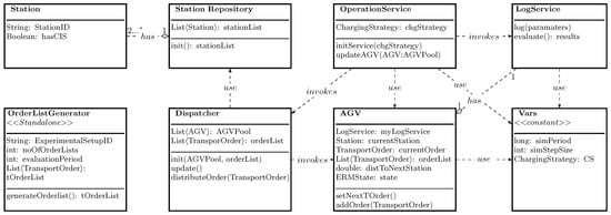
Figure 5.
UML-based software module diagram for ERM simulation. *: unlimited.
The class contains constant simulation parameters that are needed for the simulation. These include the evaluation period , the simulation step size , the applied charging strategy, and the state power parameters (cf. Section 3.4). The class consists of the parameters described in Section 3.4 as well as the variables listed in Figure 5. They are initialized instancing from the same named parameters from the class. Furthermore, AGV contains a separate function for each state presented in Section 3.5, where the parameters of the subclasses , , , and are updated each time the corresponding state functions are called by . contains a list of all stations of the current material flow and layout composition. The stations consist of the parameters and . If a has a charging station, is true; otherwise, it is false. The main process is programmed to run in cycles. Compared to an event-based simulation, a cycle-based simulation offers the opportunity for the parallel time recording of the power and energy data of the individual AGVs. This simplifies the calculation of the power requirement, which is time-dependent as mentioned in Section 3.6. Furthermore, the centrally programmed dispatching is able to allocate it considering the vehicle capacity utilization. The simulation cycle runs with a step size of from class for the duration of (equivalent to the evaluation period t in Section 3.6). Before the main cycle starts, of the class and of the class are called. Next, a central pool of similar AGVs is initialized. Afterwards the main process begins, in which, at each simulation time step, first the method of the and then are called for each of the .
4.2.1. Dispatcher
The method of the dispatcher checks whether the timestamp of a transport order on the matches or is lower than the current simulation time. If one of these cases occurs, the order or orders are transferred to the vehicles of the central . Only the current transport costs, defined by the remaining transport distances of all orders in the of an AGV, are taken into account for order assignment. The vehicle with the lowest capacity utilization is assigned the order unless the destination station of the last transport order from the matches the start station of the order to be assigned. If this matches for several vehicles, the order is assigned to the lowest utilization among these vehicles. If the utilization among these vehicles matches, the order is finally assigned according to the of the vehicle. The order allocation is performed by calling the function of the chosen AGV from the central pool.
4.2.2. OperationService
The method of updates all vehicles of the vehicle pool, including the current transport order, the remaining distance to the target station, the current state and its corresponding power requirement, the current speed, and the current SoC. Depending on the current state of the vehicle, the power requirement of the system components (cf. Section 3.1), the current speed, and the distance to the next station are recalculated. If and the state dock is completed, the current station will be overwritten with the end station of the current transport order. Afterwards, is called. The current transport order is overwritten with the next order of the local . If the list does not contain any orders, will be reset. As long as no new is assigned to the vehicle, it remains in the standby state. At the end of the method, the method of the AGV-associated instance of is called.
4.2.3. LogService
After the completion of a main cycle, is called for all from all AGVs in the central pool. Parameters like load, total distance, number of orders, and others are determined. The results of the simulations are then stored in .csv files.
4.2.4. OrderListGeneration
To ensure that experiments are under statistically reproducible conditions, transport order lists are generated following uniformly distributed order arrival times. As depicted in Figure 5, the OrderListGenerator is a standalone application that makes use of the same classes as in the simulation. The first loop of the function creates the transport orders based on the job list generated from the transport and distance matrices of the corresponding MLCs as described in [41]. The guaranteed transport orders are created as equal to the whole part of each frequency , which can be calculated as , where is valid. The fractional part represents the residual frequency , [0,1) in the corresponding hour t. The remaining frequency is then used, as the probability that another transport order of the same type will be created within the same hour is created under the condition that . In the second step, the new residual frequency for the next hour is calculated based on the following rule:
Finally, the transport order list is sorted by the timestamp of the orders. The experimental setup for AMR Karis only allowed for order batches with a reoccurring sequence. This ensures that the source stations of the current order have a load ready to pick up and the sink stations are free to drop off the load. Hence, only the inter-arrival times of the batches within each hour are varied.
4.3. ERM Input and Output
Once the transport order lists have been created, the model can be executed, provided that all necessary vehicle-specific parameters are known. These are summarized in the input–model–output Figure 6.
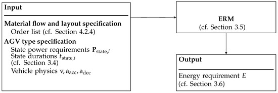
Figure 6.
Input–model–output diagram for the ERM.
5. Verification and Validation
This section presents the verification of the ERM through qualitative process analysis, followed by a description of the quantitative validation.
5.1. Qualitative Process Analysis
To demonstrate the validity of the state-based ERM (cf. Section 3.5, Figure 4), a qualitative process analysis was performed over 25 AGVs of different types from various manufacturers. For this purpose, publicly available video material was analyzed (cf. Table A3). Among all 25 AGVs, the Prepare docking state was observed in 21 AGVs. Within these 21, 10 initialized their LHD during this state for subsequent docking. The prepare driving state was observed in 20 AGVs. Among these, seven AGVs initialized their LHD in this state for subsequent driving. In total, the states Dock, Loadhandling pick up, Loadhandling drop off, and Undock were observed in 22 AGVs. The three remaining vehicles had no active LHD. Based on the results of this qualitative analysis, it is assumed that the state-based ERM is valid for AGVs of diverse configurations. If an AGV is missing any of the established process steps, the respective duration time is set to zero in the ERM. This ensures the functionality of the model for each vehicle-specific process.
5.2. Quantitative Validation
Further, the ERM is validated by comparison with experimental energy consumption measurement data. For this purpose, experiments were performed on two different types of AGVs. The experiments were equally performed by the simulation model described in Section 4. After evaluation of the experiments and the simulations, the average hourly energy requirements of the individual system components, as well as of the entire system, were compared. Two industrial used AGVs were available for the experiments, as shown in Figure 7.
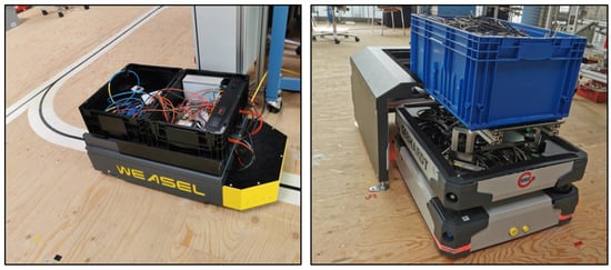
Figure 7.
Industrial used AGVs Weasel (left) and Karis (right) used in real experiments.
The vehicles differ in their chassis geometry, load-handling device, and navigation type, as well as their type of energy supply. A video of the tests with the KARIS vehicle is available as Supplemental Material.
5.2.1. Variation Parameters
As described in Section 3.3, it was assumed that the speed of the vehicle, as well as the load to be transported and the transport distance or transport time, have an effect on energy consumption. Furthermore, it was expected that the utilization of the vehicles and the charging strategy used would have a major impact on energy consumption. For this reason, in the experiments described below, speed, charging strategy, load-handling durations, vehicle utilization, load to be transported, transport layout, and the number and distribution of transport orders were varied. Within the two different vehicles, three different ESSs were used.
5.2.2. Design of Experiments
Table 3 shows the parameters of the corresponding experimental setups. For AGV Weasel, in ExperimentalSetup01A to EpxerimentalSetup01C, the speed was varied for the same transport order input. Between these, ExperimentalSetup02, and the following experimental setups, the load-handling time was varied. From ExperimentalSetup03 to ExperimentalSetup06, the charging strategy interim was evaluated by varying the utilization of the vehicle as well as the CIS frequency. In ExperimentalSetup07 to ExperimentalSetup10, the opportunity charging strategy was investigated. For this purpose, the lead–acid ESS of AGV Weasel was replaced by an EDLC ESS. Here, the utilization of the vehicle as well as the CIS frequency was also varied. The transport orders for the experiments ExperimentalSetup01A to ExperimentalSetup10 were randomly distributed as in Section 4.2.4.
Table 3.
Design of real experiments. S7 is the station with a CIS. C: capacitive, I: interim, O: opportunity. Utilization marked with * is based on simulation results.
Between ExperimentalSetup11 and ExperimentalSetup13, AMR Karis was used, varying both the vehicle load and the CIS frequency. Similarly, the flow path orientation differed as specified in [41]. The transport tasks were generated according to a fixed sequence (cf. Table A5). Depending on the workload to be achieved as seen in Table 3, these sequences were considered up to three times per hour for the creation of the transport order lists.
5.2.3. Stepsize Analysis
As described in Section 4, a discrete time simulation model was used. In order to parameterize an appropriate step size, a case study was conducted to consider the accuracies of the simulated energy requirement as the step size varied. The case study was performed on the results of ExperimentalSetup01A, which is made up of four real experiments, each 8 h in duration. The simulation of the corresponding experiments was performed with step sizes of . Figure 8 shows the variation in the relative deviation in the hourly approximated energy requirement of the drives, as well as the relative deviation in the hourly approximated energy requirement of the controls as a function of the step size s.
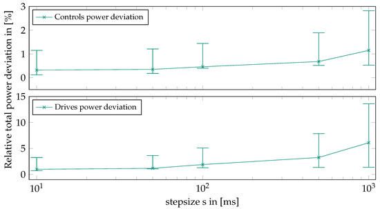
Figure 8.
Step size analysis for the discrete time simulation model.
In addition to the course of the relative deviation, the diagram also shows the lower and upper limits of the confidence interval at a significance level of . With regard to efficient simulation and a limited quality improvement at a step size of , was applied for all simulations described below.
5.2.4. Sample Size Estimation
In order to obtain significant results for the energy requirement, extended test periods are required. For this purpose, the observation period for determining the energy requirement was set to one hour. Within this hour, each vehicle-specific process (cf. Section 3.5) is run entirely at least 10 times. Again, ExperimentalSetup01A is used to determine the required sample rate per experiment. The sample size of was chosen under the assumption of a normal distribution of the results and considering a typical operation time of an AGV of . The Anderson–Darling test can be applied to the results of the study as described in [49,50]. The evaluation allows for assuming normally distributed results, which therefore will be applied to all subsequent experiments.
5.3. Experimental Setup
The experimental setup at the test area of the Institute of Material Handling and Logistics at the Karlsruhe Institute of Technology consisted of a variable transport layout, several transfer stations, charging infrastructure systems, and the two mentioned industrial used AGVs. For AGV Weasel, the experimental setup further consists of the Weasel Fleet Controller (WFC) and a custom designed charging infrastructure system. The transport layout for this vehicle was installed with optical lines on the ground and associated RFID tags, as shown in Figure 9. The CIS was installed at station S7.
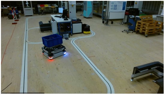
Figure 9.
Combined experimental setup for AMR Karis (left) and AGV Weasel (center), transport layout with optical track for AGV Weasel and three load transfer stations for AMR Karis.
Since AMR Karis is controlled decentrally, there is no central master control as the WFC. Compared to AGV Weasel, AMR Karis uses a manufacturer-specific CIS, which is placed at S7x. A load transfer is not possible here. Three load transfer stations are placed at S1x, S4x, and S6x. The stations S1, S4, S6, and S7 are approached, which correspond to the same stations of the AGV Weasel layout. In the case of AMR Karis, however, the docking process is added, in which the vehicle docks from the position to the corresponding station . The navigation and localization is performed by environment detection with a 2D laser scanner.
Figure 10 shows the transport layout as a representation of a directed graph. The continuous paths are visually marked routes for AGV Weasel. The path to and from station S7 is marked grey, as this is only used for charging or for jobs that start or end at S7. This represents a path with a high edge weight, which may be the case in busy traffic areas in an intralogistics environment. A virtual line is defined for AMR Karis, which is represented by a dotted line. The nodes marked with a • allow AMR Karis to leave the given virtual line in order to approach the corresponding stations.
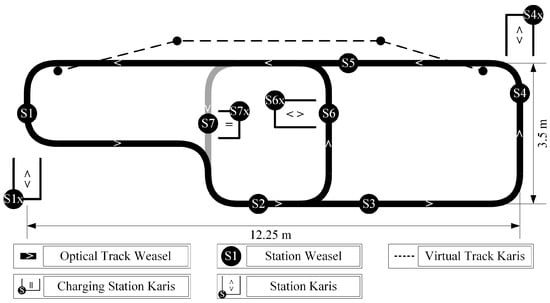
Figure 10.
Experimental layout for AGV Weasel and AMR Karis.
For both systems, a central application was developed in Java that emulates the assignment of the transport orders of the corresponding transport order lists. The application saves the start and end time of the experiments and sends transport orders into the master control (cf. WFC) or directly into the order buffer of AMR Karis. The transport orders were assigned to the vehicles as described in Section 2.3.
5.4. Measurement System
The energy measurement is performed by a measuring system of the company Klaric (cf. Figure 11).
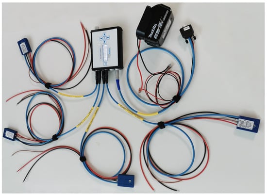
Figure 11.
Klaric measuring system with a four-channel data logger, four power probes, and an ESS-based power supply.
The measurement system consists of a KLARI-CORD 5 data logger and four LP-Probe-10mR probes for power consumption measurement. The power supply for the measurement system is provided by an external Makita battery. The data logger samples the power consumption data at a frequency of and stores the data with a compressed rate of on an external data carrier. The measurement concepts for the two vehicles fitted to the respective system components are shown in Figure A1 and Figure A2. A channel describes a probe of the type LP-Probe-10mR, measuring both the current and the voltage. If several channels were connected to the same voltage potential, the voltage was only measured with one of these channels in order to minimize the amount of data to be stored. The measurement system also includes a temperature data logger from Testo, type 174T, which was parameterized to a recording rate of 60 values per hour.
5.5. Experimental Data Evaluation
To evaluate the collected data of each measurement channel as well as the temperature data, they were loaded into a Matlab script. After reading the start and end timestamp from the respective experiment, the data were synchronized and trimmed to the time period to be considered.
By analyzing the measured power consumption data, it was possible to determine threshold values in the different measurement channels to identify the different process states according to Section 3.5. Subsequently, the power consumptions were divided into classes corresponding to the processes of the ERM. Each class was finally analyzed individually for process duration and average power consumption to linearize the process specific power requirements. These results are required as input parameters for the ERM. Furthermore, the average energy requirements per hour were determined. These are the values that are used as comparison parameters with the simulation model subsequently. The results of the experimental data evaluation can be found in Table A1.
6. Results
To validate the ERM and to determine its quality, 15 real experiments with two test vehicles were conducted. During these experiments, power requirement data were recorded over of operating time for AGV Weasel and of operating time for AMR Karis in total. During the experiments, AGV Weasel drove a total distance of and AMR Karis drove a total distance of .
6.1. ERM and Experiments Comparison
The experiments performed were simulated (cf. Section 4) and the results were compared. Figure 12 shows an example plot of the power consumption data of AMR Karis during a randomly selected transport cycle from ExperimentalSetup13. Starting with a load-handling dropping process (A), the system subsequently goes through the states undock (B), prepare driving (C), drive (D), prepare docking (E), dock (F), and picking (G). The prepare docking as well as dock states are repeated four times in this random cycle until the dock operation is completed. The three diagrams in Figure 12 show the power consumption of the controls, the drives, and the LHD from top to bottom. The dotted lines describe the modeled linear power requirements according to Section 3.4. The vertical black lines show the bounds of the respective states of the model (cf. Section 5.5). Since the power consumption of the drives during the drive state did not provide assignable power peaks for acceleration and deceleration, the acceleration and deceleration states were not parameterized in the simulation. The acceleration and deceleration phases were therefore implicitly taken into account by the state drive.
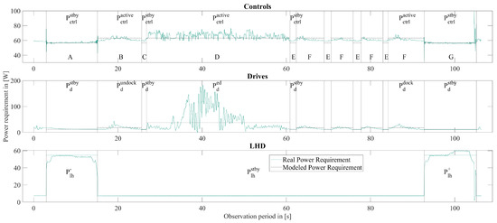
Figure 12.
Comparison of measured power consumption and modeled power requirement.
6.2. Evaluation
The quality of the model is evaluated by comparing the simulative results with the experimental results. The comparison results are the relative deviations in the average power requirements of the individual system components (cf. Section 3.1) and were calculated according to the following calculation rule:
The comparison results are hereafter referred to as samples. After assuming the normal distribution of the samples (cf. Section 5.2.4), the confidence interval procedure of [51,52] was chosen to determine the quality of the model. Based on the samples of relative deviations in energy requirements, the lower and upper bounds of the confidence intervals for the significance levels of and were set. They can be found in Table A2. In the upper part of Figure 13, the relative energy requirement deviation of the corresponding system components of AGV Weasel is shown, whereas, in the lower part, the deviations of AMR Karis can be seen. The marked points describe the corresponding mean value of all tests performed with the respective vehicle. The horizontal lines describe the limits of the confidence intervals at a significance level of .
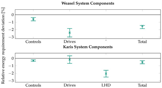
Figure 13.
System-component-dependent relative energy requirement deviation.
It can be seen that the controls were modeled within the confidence interval of to . The accuracy of the energy requirement approximation for the drives varies between the two vehicles. For AGV Weasel, the confidence interval is in the range of to , whereas, for AMR Karis, the confidence interval is in the range of to . Due to the technical equipment, the energy requirement of the LHD could only be investigated for AGV Karis. The relative deviation in the energy requirement of the LHD lies in the confidence interval of to . Overall, the total energy requirements of AGV Weasel was determined within a confidence interval of to and, for AMR Karis, within a confidence interval of to , each at a significance level of . These, as well as the results of each individual experiment and for a further significance level of , can be found in Table A2.
6.3. Discussion
The results show that the controls could be modeled more accurately compared to the drives and the LHD. This can be attributed to environmental impacts such as friction force, as [10,16] have shown. Furthermore, the modeling of the drives for AMR Karis was more accurate than that of AGV Weasel. One possible explanation for this is that the rated power of the drives of AGV Weasel is only about one-third of the rated power of the drives of AMR Karis. Environmental impact, such as the friction force mentioned earlier, may have a greater relative impact on the power required here. In most cases, the energy requirement was underestimated.
Furthermore, necessary assumptions for the experimental setups were made. Concerning the real experiments, the CISs were always installed directly at load transfer stations, which is valid for experiments with charging strategies I and O. A charging process always starts simultaneously with a load-handling process. For the implementation of the dispatching method for real experiments and simulations, each transport order starts with a load pickup and ends with a load delivery, and a load-handling process is not performed during empty runs. In addition to the assumptions, one of the limitations of the ERM is, that since a linear power approximation is performed in the ERM, efficiencies of DCDCs as well as acceleration and deceleration cannot be specified as a functional quantity. Further, the ERM cannot consider possible collisions or traffic rules of AGVs, which are further assumed to be single-load. Finally, the ERM cannot consider the influencing factors of various ESSs and CISs. The process analysis of 25 different AGVs was conducted to make an initial statement about the applicability of the EDM for different AGVs. For more general statements, however, further vehicle types need to be analyzed, and more detailed delimitations of the model need to be defined in case of possible deviations.
The EDM was validated based on real experiments with two different industrial used vehicles with a maximum average total power consumption while driving of and a maximum average power of the LHD in the active load-handling state of . More real experiments with AGVs of higher power classes, such as forklift AGVs, are required to make a more general statement on the applicability of the model. Longer experiments are also required to validate the long-term reliability of the model concerning continuous operation times for more than 24 h.
6.4. Further Findings
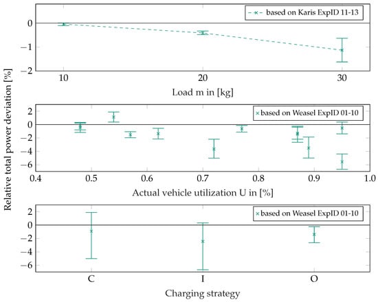
Figure 14.
Relative power requirement accuracy deviation contrasted by various experiment parameters.
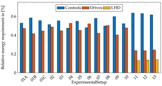
Figure 15.
Relative energy requirements of each system component at experiments (01A to 10) for AGV Weasel and at experiments (11 to 13) for AMR Karis.
Figure 14 shows the impact of the three factors of load, vehicle utilization, and charging strategy on the relative total energy deviation. Considering the influencing factor load, it can be seen that the accuracy of the energy requirement approximation decreases with an increasing load. The width of the confidence interval also widens. Except for one case, it can be seen that the accuracy decreases with an increasing utilization and the width of the confidence intervals also widens. In the bottom graph, it can be seen that the experiments with the charging strategy opportunity (O) could be estimated with an interval of to , followed by the capacitive (C) charging strategy with an interval of to . The experiments with the charging strategy interim (I) have estimated it as the worst, with an interval of to , where all intervals consider the minimum lower limit and maximum upper limit of the confidence intervals of the respective experiments. Another finding is the unexpected impact of the controls on the total energy requirement of an AGV. In contrast to the studies mentioned in the literature review (cf. Section 2), controls also have a major impact on the total energy consumption of an AGV. Figure 15 shows the relative energy requirements of each system component in an AGV.
Figure 15 shows the relative energy consumption of AGV Weasel for ExperimentalSetup01A to ExperimentalSetup10. On average, the controls make up and the drives make up of the total energy consumption. This is also shown for AMR Karis with ExperimentalSetup11 to ExperimentalSetup13. On average, the controls make up , the drives make up , and the LHD makes up of the total energy consumption.
7. Conclusions
In this study, an ERM for AGVs was presented. The state-based model was verified by a comprehensive process analysis and validated with real experiments, and therefore allows for accurate estimation of the energy requirement of AGVs under multiple constraints. The model has mean estimation accuracies of energy requirements at a significance level of of approximately . These models were validated only on test vehicles and not on real vehicles used in industry. This provides opportunities to estimate the energy requirement of AGVs in advance, considering influencing factors. This can be used to derive possible energy efficiency measures or to optimize the design of ESSs for AGVs. Although this model provides accurate energy requirement estimations for the two vehicle types studied, further investigations are needed to establish the generality of this model. This will require the analysis of additional vehicle types and the definition of more detailed model delimitations in the case of possible deviation. It is assumed that the state-based model can be extended for more complex system behaviors if required. Similarly, it is assumed that this can be applied to the energy requirement modeling of storage shuttle systems through adjustments to the process steps of the ERM.
To validate these statements, further investigations are needed, validated with real-world experiments, such as real-world experiments and measurements on storage shuttle systems. As Chang et al. [53] show, the transport orders for public transit buses can be planned in the same way as for AGVs. This allows for further investigation into the calculation of energy requirements for battery-powered transit buses. Finally, based on this work, the energy storage requirements of AGVs can be modeled in future work. In addition to the vehicle’s energy requirement, the maximum operating time, the frequency of charging operations, the distribution of the charging infrastructure systems in the layout, and the charging strategy will also be considered.
Supplementary Materials
The following supporting information can be downloaded at: https://www.mdpi.com/article/10.3390/designs8030048/s1. Video demonstrating experiments with KARIS; Measurement and evaluation data of all experiments; Anderson-Darling-Test showing normal distibution of the results.
Author Contributions
M.S.: conceptualization, methodology, formal analysis, investigation, resources, software, data curation, writing—original draft preparation, writing—review and editing, visualization. K.F.: writing—review and editing, supervision, management and coordination responsibility for the research activity planning and execution. All authors have read and agreed to the published version of the manuscript.
Funding
This research was funded by the German Federal Ministry for Economic Affairs and Energy under the grant number KK5040304ZG0.
Institutional Review Board Statement
Not applicable.
Informed Consent Statement
Not applicable.
Data Availability Statement
The research data supporting this study are available in additional .csv files provided as Supplementary Material. Additionally, tables containing relevant data are presented in the Appendix A of this article.
Acknowledgments
We acknowledge support from the KIT-Publication Fund of the Karlsruhe Institute of Technology. Thanks to the students Yarkin Doruk Dogan, Jacqueline Stefanie Kaefer, Lacin Kertmen, Johannes Pfeifer, Ibrahim Bouriga, Lena Susanne Schmidt, and Mark Rauh for their contributions. Thanks to Pietro Schumacher for his review. Special thanks to the companies Ansmann AG for providing the ELDC Module, Klaric for providing the measurement system, SSI Schäfer for providing the AGV Weasel test vehicle, and Things Alive Robotics for providing the AMR Karis test vehicle.
Conflicts of Interest
The authors declare no conflicts of interest.
Abbreviations
The following abbreviations are used in this manuscript:
| AGV | Automated Guided Vehicle |
| AMR | Autonomous Mobile Robot |
| C | Charging Strategy Capacitive |
| CIS | Charging Infrastructure System |
| ESS | Energy Storage System |
| I | Charging Strategy Interim |
| LHD | Load-Handling Device |
| O | Charging Strategy Opportunity |
| ERM | Energy Requirement Model |
Appendix A
Table A1.
Simulation parameter for model validation, based on measured experimental data.
Table A1.
Simulation parameter for model validation, based on measured experimental data.
| ExpID | Physics | Times | Powers in [W] | ||||||||||||||||
|---|---|---|---|---|---|---|---|---|---|---|---|---|---|---|---|---|---|---|---|
| in [m/s, m/s2, m/s2] | in [s] | Charge | LHD | Controls | Drives | ||||||||||||||
| 01A | 1.0 | 1.0 | 1.0 | 5.0 | - | - | - | - | - | - | - | 7.480 | 5.480 | 39.179 | 12.478 | −14.287 | 1.578 | - | - |
| 01B | 0.5 | 1.0 | 1.0 | 5.0 | - | - | - | - | - | - | - | 7.414 | 5.476 | 26.747 | 6.204 | −6.278 | 1.678 | - | - |
| 01C | 0.7 | 1.0 | 1.0 | 5.0 | - | - | - | - | - | - | - | 7.245 | 5.469 | 30.405 | 8.451 | −9.997 | 1.688 | - | - |
| 2 | 1.0 | 1.0 | 1.0 | 15.0 | - | - | - | - | - | - | - | 7.371 | 5.455 | 39.772 | 12.640 | −14.384 | 1.644 | - | - |
| 3 | 1.0 | 1.0 | 1.0 | 10.0 | - | - | - | - | 75.591 | - | - | 7.430 | 5.457 | 40.080 | 13.008 | −14.338 | 1.685 | - | - |
| 4 | 1.0 | 1.0 | 1.0 | 10.0 | - | - | - | - | 72.159 | - | - | 7.329 | 5.451 | 39.615 | 12.901 | −14.284 | 1.601 | - | - |
| 5 | 1.0 | 1.0 | 1.0 | 10.0 | - | - | - | - | 65.292 | - | - | 7.492 | 5.459 | 40.822 | 13.380 | −14.370 | 1.770 | - | - |
| 6 | 1.0 | 1.0 | 1.0 | 10.0 | - | - | - | - | 73.190 | - | - | 7.520 | 5.457 | 41.282 | 12.928 | −13.931 | 1.629 | - | - |
| 7 | 1.0 | 1.0 | 1.0 | 10.0 | - | - | - | - | 92.626 | - | - | 7.363 | 5.480 | 38.175 | 12.756 | −13.144 | 1.917 | - | - |
| 8 | 1.0 | 1.0 | 1.0 | 10.0 | - | - | - | - | 109.986 | - | - | 7.350 | 5.472 | 38.220 | 12.998 | −13.136 | 1.884 | - | - |
| 9 | 1.0 | 1.0 | 1.0 | 10.0 | - | - | - | - | 52.696 | - | - | 7.338 | 5.477 | 38.987 | 13.103 | −13.210 | 1.970 | - | - |
| 10 | 1.0 | 1.0 | 1.0 | 10.0 | - | - | - | - | 62.658 | - | - | 7.403 | 5.479 | 38.785 | 12.892 | −13.212 | 1.954 | - | - |
| 11 | 0.25 | 0.4 | 1.0 | 10.735 | 3.664 | 17.626 | 9.356 | 0.924 | 1415.0 | 52.254 | 7.339 | 62.961 | 57.271 | - | 36.021 | - | 10.797 | 17.625 | 17.986 |
| 12 | 0.27 | 0.4 | 1.0 | 9.330 | 3.580 | 18.202 | 9.951 | 0.795 | 1415.0 | 54.511 | 7.455 | 62.920 | 55.814 | - | 37.614 | - | 10.913 | 18.160 | 18.488 |
| 13 | 0.28 | 0.4 | 1.0 | 8.667 | 3.436 | 15.708 | 9.693 | 0.870 | 1365.0 | 54.716 | 7.504 | 63.193 | 55.152 | - | 37.897 | - | 11.651 | 18.067 | 18.235 |
Table A2.
System components energy requirement deviation between simulation and real experiments, presented as confidence intervals for specific significance levels .
Table A2.
System components energy requirement deviation between simulation and real experiments, presented as confidence intervals for specific significance levels .
| ExpID | Max. rel. Deviation Controls | Max. rel. Deviation Drives | Max. rel. Deviation LHD | Max. rel. Deviation All Components | ||||||||||||
|---|---|---|---|---|---|---|---|---|---|---|---|---|---|---|---|---|
| α = 1% | α = 5% | α = 1% | α = 5% | α = 1% | α = 5% | α = 1% | α = 5% | |||||||||
| Δlow | Δhigh | Δlow | Δhigh | Δlow | Δhigh | Δlow | Δhigh | Δlow | Δhigh | Δlow | Δhigh | Δlow | Δhigh | Δlow | Δhigh | |
| 01A | - | - | - | - | ||||||||||||
| 01B | - | - | - | - | ||||||||||||
| 01C | - | - | - | - | ||||||||||||
| 02 | - | - | - | - | ||||||||||||
| 03 | - | - | - | - | ||||||||||||
| 04 | - | - | - | - | ||||||||||||
| 05 | - | - | - | - | ||||||||||||
| 06 | - | - | - | - | ||||||||||||
| 07 | - | - | - | - | ||||||||||||
| 08 | - | - | - | - | ||||||||||||
| 09 | - | - | - | - | ||||||||||||
| 10 | - | - | - | - | ||||||||||||
| All Weasel | - | - | - | - | ||||||||||||
| 11 | ||||||||||||||||
| 12 | ||||||||||||||||
| 13 | ||||||||||||||||
| All Karis | ||||||||||||||||
Table A3.
Qualitative Process Analysis of Industrial AGVs. (x): Considered. (-): Not considered.
Table A3.
Qualitative Process Analysis of Industrial AGVs. (x): Considered. (-): Not considered.
| Nr | LHD | AGV Name | Process | Prepare Docking | Dock | LH | Undock | Prepare Driving | Source | ||
|---|---|---|---|---|---|---|---|---|---|---|---|
| Stop | Init LHD | Stop | Init LHD | ||||||||
| 1 | tug | Jungheinrich EZS 350a | pick | x | - | x | x | x | - | - | [54] |
| drop | - | - | x | x | x | - | - | ||||
| 2 | fork-lift | Jungheinrich ERC 215a | pick/drop | x | x | x | x | x | x | x | [55] |
| 3 | fork-lift | Agilox One | pick/drop | x | - | x | x | x | x | - | [56] |
| charge | x | - | x | - | x | x | - | ||||
| 4 | fork-lift | Lmatic high-lift truck | pick/drop | x | x | x | x | x | - | - | [57] |
| 5 | fork-lift | TÜNKERS STacker | pick | x | x | x | x | x | x | x | [58] |
| 6 | fork-lift | K. Hartwall A-Mate | pick/drop | - | x | x | x | x | - | x | [59] |
| 7 | topload | Agilox ODM | pick | x | - | x | x | x | x | - | [60] |
| drop | x | x | x | x | x | x | - | ||||
| 8 | topload | MiR200 | pick/drop | x | - | x | x | x | x | - | [61] |
| park | x | - | x | - | x | x | - | ||||
| 9 | topload | Gebhardt Karis Custom Model | pick/drop | x | x | x | x | x | x | x | - |
| charge | x | - | x | - | x | x | - | ||||
| 10 | topload | Jungheinrich AMR arculee S | pick/drop | x | - | x | x | x | x | [62] | |
| 11 | topload | Idealworks iw.hub | pick/drop | x | - | x | x | x | x | - | [63] |
| 12 | topload | Milvus Robotics SEIT500 | pick | x | - | x | x | x | x | x | [64] |
| drop | x | x | x | x | x | x | - | ||||
| 13 | topload | Grenzebach L600-Li | pick/drop | x | x | x | x | x | [65] | ||
| 14 | topload | Safelog X1 | pick/drop | x | - | x | x | x | x | - | [66] |
| 15 | topload | Bosch Activeshuttle | pick/drop | x | x | x | x | x | x | x | [67] |
| 16 | passive | Mir 250 | pick/drop | x | - | x | x | x | x | - | [68] |
| 17 | passive | SSI Schäfer Weasel Lite | pick/drop | - | - | - | - | - | x | - | [69] |
| 18 | passive | SSI Schäfer Weasel | pick | x | - | - | - | - | - | - | [70] |
| drop | - | - | - | - | - | x | - | ||||
| 19 | passive | BITO FTS Leo | pick/drop | - | - | - | - | - | - | - | [71] |
| 20 | roller conveyor | DS Automation Sally | pick/drop | x | - | x | x | x | x | - | [72] |
| 21 | roller conveyor | Carrybots Herbie | pick/drop | - | - | x | x | x | - | - | [73] |
| 22 | roller conveyor | SHERPA-B | pick/drop | - | - | x | x | x | - | - | [74] |
| 23 | roller conveyor | Omron LD-60/90 | pick/drop | x | - | x | x | x | x | - | [75] |
| 24 | roller conveyor | Gebhardt Karis Model 3 | pick/drop | x | x | x | x | x | x | - | [76] |
| 25 | customized lift | Gessbot Gb350 | drop | x | x | x | x | x | x | x | [77] |
Table A4.
Technical specifications of the AGVs.
Table A4.
Technical specifications of the AGVs.
| Weasel | Karis | |
|---|---|---|
| Manufacturer | SSI Schaefer | Gebhardt Fordertechnik |
| Mass (vehicle without load) | ||
| Mass (load) | - | |
| Dimensions (vehicle without load, l × w × h) | × × | × × |
| Nominal system voltage | , | |
| Battery | Lead–acid Battery, EDLC | Varta Easy Blade 48 V |
Table A5.
Material flow and layout description of the experiments.
Table A5.
Material flow and layout description of the experiments.
| Exp. ID | AGVID | Representation of Material Flow and Layout | Material Flow and Layout Classification | |||
|---|---|---|---|---|---|---|
| Layout | Material Flow per Hour | Flow Path Orientation | Layout Topology | Task Structure | ||
| 01A 01B 01C 02 | Weasel | 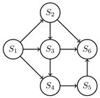 | unidir. | multiloop | m:n | |
| 03 04 05 06 07 08 09 10 | Weasel | 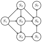 | unidir. | multiloop | m:n | |
| 11 12 | Karis |  | bidir. | multiloop | m:n | |
| 13 | Karis |  | unidir. | multiloop | m:n | |
Table A6.
Technical specifications of the used ESS.
Table A6.
Technical specifications of the used ESS.
| Lead-Acid Battery | 20S4P 400F EDLC | Easy Blade 48 | |
|---|---|---|---|
| Manufacturer | SSI Schaefer | Ansmann AG | Varta Storage GmbH |
| Version | 1.0 | 1.0 | 56654 799 092 |
| Cell type | 2xYuasa NP12-12 | Cornell Dubilier DSF407Q3R0 | N.A. |
| Mass | |||
| Dimensions (l × w × h) | × × | × × | × × |
| Nominal Voltage | |||
| Maximum Current | () | ||
| Nominal Crate Charging | |||
| Nominal E |
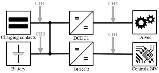
Figure A1.
AGV Weasel power consumption measurement concept.
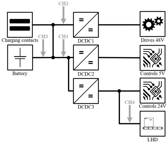
Figure A2.
AMR Karis power consumption measurement concept.
References
- Official Journal of the European Union. Directive (EU) 2023/1791 of the European Parliament and of the Council of 13 September 2023 on Energy Efficiency and Amending REGULATION (EU) 2023/955 (Recast); Official Journal of the European Union: Luxembourg, 2023. [Google Scholar]
- Freis, J.; Günthner, W.A. A systemic approach to analysing interactions and impacts of alternative design options on the total energy balance of distribution warehouses. Wiss. Ges. Tech. Logist. 2016. [Google Scholar] [CrossRef]
- Müller, E.; Hopf, H.; Krones, M. Analyzing Energy Consumption for Factory and Logistics Planning Processes. In Advances in Production Management Systems. Competitive Manufacturing for Innovative Products and Services; Emmanouilidis, C., Taisch, M., Kiritsis, D., Eds.; IFIP Advances in Information and Communication Technology; Springer: Berlin/Heidelberg, Germany, 2013; Volume 397, pp. 49–56. [Google Scholar] [CrossRef]
- Ebben, M. Logistic Control in Automated Transportation Networks; Twente Univ. Press: Enschede, The Netherlands, 2001. [Google Scholar]
- IEC 62264-1:2013; Enterprise-Control System Integration—Part 1: Models and Terminology. International Electrotechnical Commission: Geneva, Switzerlandm, 2013.
- Mei, Y.; Lu, Y.H.; Hu, Y.C.; Lee, C. Deployment of mobile robots with energy and timing constraints. IEEE Trans. Robot. 2006, 22, 507–522. [Google Scholar] [CrossRef]
- Qiu, L.; Wang, J.; Chen, W.; Wang, H. Heterogeneous AGV routing problem considering energy consumption. In Proceedings of the 2015 IEEE International Conference on Robotics and Biomimetics (ROBIO), Zhuhai, China, 6–9 December 2015; IEEE: Piscataway, NJ, USA; pp. 1894–1899. [Google Scholar] [CrossRef]
- Kim, C.H.; Kim, B.K. Minimum-Energy Translational Trajectory Generation for Differential-Driven Wheeled Mobile Robots. J. Intell. Robot. Syst. 2007, 49, 367–383. [Google Scholar] [CrossRef]
- Kim, H.; Kim, B.K. Minimum-energy translational trajectory planning for battery-powered three-wheeled omni-directional mobile robots. In Proceedings of the 2008 10th International Conference on Control, Automation, Robotics and Vision, Hanoi, Vietnam, 17–20 December 2008; IEEE: Piscataway, NJ, USA; pp. 1730–1735. [Google Scholar] [CrossRef]
- Liu, S.; Sun, D. Minimizing Energy Consumption of Wheeled Mobile Robots via Optimal Motion Planning. IEEE/ASME Trans. Mechatron. 2014, 19, 401–411. [Google Scholar] [CrossRef]
- Kabir, Q.S.; Suzuki, Y. Comparative analysis of different routing heuristics for the battery management of automated guided vehicles. Int. J. Prod. Res. 2019, 57, 624–641. [Google Scholar] [CrossRef]
- Stampa, M.; Rohrig, C.; Kunemund, F.; Hes, D. Estimation of energy consumption on arbitrary trajectories of an omnidirectional automated guided vehicle. In Proceedings of the 2015 IEEE 8th International Conference on Intelligent Data Acquisition and Advanced Computing Systems: Technology and Applications (IDAACS), Warsaw, Poland, 24–26 September 2015; IEEE: Piscataway, NJ, USA; pp. 873–878. [Google Scholar] [CrossRef]
- Hou, L.; Zhang, L.; Kim, J. Energy Modeling and Power Measurement for Mobile Robots. Energies 2019, 12, 27. [Google Scholar] [CrossRef]
- Niestrój, R.; Rogala, T.; Skarka, W. An Energy Consumption Model for Designing an AGV Energy Storage System with a PEMFC Stack. Energies 2020, 13, 3435. [Google Scholar] [CrossRef]
- Hamdy, A. Optimization of Automated Guided Vehicles (AGV) Fleet Size with Incorporation of Battery Management. Ph.D. Thesis, Old Dominion University Libraries, Norfolk, VA, USA, 2019. [Google Scholar] [CrossRef]
- Meißner, M.; Massalski, L. Modeling the electrical power and energy consumption of automated guided vehicles to improve the energy efficiency of production systems. Int. J. Adv. Manuf. Technol. 2020, 110, 481–498. [Google Scholar] [CrossRef]
- McHaney, R. Modelling battery constraints in discrete event automated guided vehicle simulations. Int. J. Prod. Res. 1995, 33, 3023–3040. [Google Scholar] [CrossRef]
- Singh, N.; Dang, Q.V.; Akcay, A.; Adan, I.; Martagan, T. A matheuristic for AGV scheduling with battery constraints. Eur. J. Oper. Res. 2022, 298, 855–873. [Google Scholar] [CrossRef]
- Abderrahim, M.; Bekrar, A.; Trentesaux, D.; Aissani, N.; Bouamrane, K. Manufacturing 4.0 Operations Scheduling with AGV Battery Management Constraints. Energies 2020, 13, 4948. [Google Scholar] [CrossRef]
- Colling, D.; Oehler, J.; Furmans, K. Battery Charging Strategies for AGV Systems. Wiss. Ges. Tech. Logist. 2019. [Google Scholar] [CrossRef]
- Zhan, X.; Xu, L.; Zhang, J.; Li, A. Study on AGVs battery charging strategy for improving utilization. Procedia CIRP 2019, 81, 558–563. [Google Scholar] [CrossRef]
- Jodejko-Pietruczuk, A.; Werbinska-Wojciechowska, S. Availability assessment for a multi-AGV system based on simulation modeling approach. In Proceedings of the 2021 International Conference on Electrical, Computer, Communications and Mechatronics Engineering (ICECCME), Mauritius, Mauritius, 7–8 October 2021; IEEE: Piscataway, NJ, USA; pp. 1–6. [Google Scholar] [CrossRef]
- Quadrini, W.; Negri, E.; Fumagalli, L. Open Interfaces for Connecting Automated Guided Vehicles to a Fleet Management System. Procedia Manuf. 2020, 42, 406–413. [Google Scholar] [CrossRef]
- Sperling, M.; Kivelä, T. Concept of a Dual Energy Storage System for Sustainable Energy Supply of Automated Guided Vehicles. Energies 2022, 15, 479. [Google Scholar] [CrossRef]
- VDI Society Production and Logistics. Automated Guided Vehicle Systems (AGVS)—Power Supply and Charging Technology; VDI Society Production and Logistics: Düsseldorf, Germany, 2022. [Google Scholar]
- VDI Society Production and Logistics. Compatibility of Automated Guided Vehicle Systems (AGVS)—Power Supply and Charging Technology; VDI Society Production and Logistics: Düsseldorf, Germany, 2000. [Google Scholar]
- de Ryck, M.; Pissoort, D.; Holvoet, T.; Demeester, E. Decentral task allocation for industrial AGV-systems with routing constraints. J. Manuf. Syst. 2022, 62, 135–144. [Google Scholar] [CrossRef]
- Fragapane, G.; de Koster, R.; Sgarbossa, F.; Strandhagen, J.O. Planning and control of autonomous mobile robots for intralogistics: Literature review and research agenda. Eur. J. Oper. Res. 2021, 294, 405–426. [Google Scholar] [CrossRef]
- Vivaldini, K.C.T.; Rocha, L.F.; Becker, M.; Moreira, A.P. Comprehensive Review of the Dispatching, Scheduling and Routing of AGVs. In CONTROLO’2014—Proceedings of the 11th Portuguese Conference on Automatic Control; Lecture Notes in Electrical Engineering; Moreira, A.P., Matos, A., Veiga, G., Eds.; Springer International Publishing: Cham, Switzerland, 2015; Volume 321, pp. 505–514. [Google Scholar] [CrossRef]
- Zamiri Marvizadeh, S.; Choobineh, F.F. Entropy-based dispatching for automatic guided vehicles. Int. J. Prod. Res. 2014, 52, 3303–3316. [Google Scholar] [CrossRef]
- Yang, X.G.; Wang, C.Y. Understanding the trilemma of fast charging, energy density and cycle life of lithium-ion batteries. J. Power Sources 2018, 402, 489–498. [Google Scholar] [CrossRef]
- Gao, Z.; Xie, H.; Yang, X.; Niu, W.; Li, S.; Chen, S. The Dilemma of C-Rate and Cycle Life for Lithium-Ion Batteries under Low Temperature Fast Charging. Batteries 2022, 8, 234. [Google Scholar] [CrossRef]
- Stroe, A.I.; Stroe, D.L.; Knap, V.; Swierczynski, M.; Teodorescu, R. Accelerated Lifetime Testing of High Power Lithium Titanate Oxide Batteries. In Proceedings of the 2018 IEEE Energy Conversion Congress and Exposition (ECCE), Portland, OR, USA, 23–27 September 2018; IEEE: Piscataway, NJ, USA; pp. 3857–3863. [Google Scholar] [CrossRef]
- Leuchter, J.; Bauer, P. Capacity of power-batteries versus temperature. In Proceedings of the 2015 17th European Conference on Power Electronics and Applications (EPE’15 ECCE-Europe), Geneva, Switzerland, 8–10 September 2015; IEEE: Piscataway, NJ, USA; pp. 1–8. [Google Scholar] [CrossRef]
- Vidal, C.; Gross, O.; Gu, R.; Kollmeyer, P.; Emadi, A. xEV Li-Ion Battery Low-Temperature Effects—Review. IEEE Trans. Veh. Technol. 2019, 68, 4560–4572. [Google Scholar] [CrossRef]
- Wood, E.; Alexander, M.; Bradley, T.H. Investigation of battery end-of-life conditions for plug-in hybrid electric vehicles. J. Power Sources 2011, 196, 5147–5154. [Google Scholar] [CrossRef]
- Saldaña, G.; San Martín, J.I.; Zamora, I.; Asensio, F.J.; Oñederra, O. Analysis of the Current Electric Battery Models for Electric Vehicle Simulation. Energies 2019, 12, 2750. [Google Scholar] [CrossRef]
- Hu, X.; Le, X.; Lin, X.; Pecht, M. Battery Lifetime Prognostics. Joule 2020, 4, 310–346. [Google Scholar] [CrossRef]
- Devillers, N.; Jemei, S.; Péra, M.C.; Bienaimé, D.; Gustin, F. Review of characterization methods for supercapacitor modelling. J. Power Sources 2014, 246, 596–608. [Google Scholar] [CrossRef]
- Yang, H. Effects of Aging and Temperature on Supercapacitor Charge Capacity. In Proceedings of the 2020 IEEE Power & Energy Society General Meeting (PESGM), Montreal, QC, Canada, 2–6 August 2020; IEEE: Piscataway, NJ, USA; pp. 1–5. [Google Scholar] [CrossRef]
- Sperling, M.; Schulz, B.; Enke, C.; Giebels, D.; Furmans, K. Classified AGV Material Flow and Layout Data Set for Multidisciplinary Investigation. IEEE Access 2023, 11, 94992–95007. [Google Scholar] [CrossRef]
- Hanschek, A.J.; Bouvier, Y.E.; Jesacher, E.; Grbovic, P.J. Analysis of power distribution systems based on low-voltage DC/DC power supplies for automated guided vehicles (AGV). In Proceedings of the 2021 21st International Symposium on Power Electronics (Ee), Novi Sad, Serbia, 27–30 October 2021; IEEE: Piscataway, NJ, USA; pp. 1–6. [Google Scholar] [CrossRef]
- Arbetter, B.; Erickson, R.; Maksimovic, D. DC-DC converter design for battery-operated systems. In Proceedings of the PESC’95—Power Electronics Specialist Conference, Atlanta, GA, USA, 18–22 June 1995; IEEE: Piscataway, NJ, USA; pp. 103–109. [Google Scholar] [CrossRef]
- Komma, V.R.; Jain, P.K.; Mehta, N.K. Simulation of AGV System—A Multi Agent Approach. In DAAAM International Scientific Book 2012; Katalinic, B., Ed.; DAAAM International: Vienna, Austria, 2012. [Google Scholar] [CrossRef]
- Flake, S. UML-Based Specification of State Oriented Real Time Properties. Ph.D. Thesis, Paderborn University, Paderborn, Germany, 2003. [Google Scholar]
- Cebrian, J.M.; Natvig, L. Temperature effects on on-chip energy measurements. In Proceedings of the 2013 International Green Computing Conference Proceedings, Arlington, VA, USA, 27–29 June 2013; IEEE: Piscataway, NJ, USA; pp. 1–6. [Google Scholar] [CrossRef]
- Eggers, K.; Knochelmann, E.; Tappe, S.; Ortmaier, T. Modeling and experimental validation of the influence of robot temperature on its energy consumption. In Proceedings of the 2018 IEEE International Conference on Industrial Technology (ICIT), Lyon, France, 20–22 February 2018; IEEE: Piscataway, NJ, USA; pp. 239–243. [Google Scholar] [CrossRef]
- Zhai, N.; Yao, Y.; Zhang, D.; Xu, D. Design and Optimization for a Supercapacitor Application System. In Proceedings of the 2006 International Conference on Power System Technology, Chongqing, China, 22–26 October 2006; IEEE: Piscataway, NJ, USA; pp. 1–4. [Google Scholar] [CrossRef]
- Dodge, Y. Anderson–Darling Test. In The Concise Encyclopedia of Statistics; Springer: New York, NY, USA, 2008; pp. 12–14. [Google Scholar] [CrossRef]
- Berlinger, M. A Methodology to Model the Statistical Fracture Behavior of Acrylic Glasses for Stochastic Simulation; Springer: Wiesbaden, Germany, 2021; Volume 59. [Google Scholar] [CrossRef]
- Schiefer, H.; Schiefer, F. Statistics for Engineers: An Introduction with Examples from Practice; Springer: Wiesbaden/Heidelberg, Germany, 2021. [Google Scholar] [CrossRef]
- Plaue, M. Data Science: An Introduction to Statistics and Machine Learning, 1st ed.; Springer: Berlin/Heidelberg, Germany, 2023. [Google Scholar] [CrossRef]
- Chang, A.; Cong, Y.; Wang, C.; Bie, Y. Optimal Vehicle Scheduling and Charging Infrastructure Planning for Autonomous Modular Transit System. Sustainability 2024, 16, 3316. [Google Scholar] [CrossRef]
- Jungheinrich, A.G. Der Automatisierte Schlepper zur Effizienten Produktionsversorgung: Jungheinrich EZSa. 2021. Available online: https://www.youtube.com/watch?v=NBEKhpSZ7j4 (accessed on 3 January 2024).
- Jungheinrich, A.G. Fahrerlose Transportsysteme von Jungheinrich im Einsatz bei BMW Group. 2017. Available online: https://www.youtube.com/watch?v=4TInapyb3-8 (accessed on 3 January 2024).
- CLS Servizi e Soluzioni in Movimento. Agilox—Intelligent Guided Vehicle. 2020. Available online: https://www.youtube.com/watch?v=F5DoflSjiWQ (accessed on 3 January 2024).
- Linde Material Handling. Two Value-Adding Industrial Trucks at Full Speed|Linde Material Handling. 2021. Available online: https://www.youtube.com/watch?v=4fzakJh2MyY (accessed on 3 January 2024).
- TÜNKERS Maschinenbau GmbH. TÜNKERS STacker. 2022. Available online: https://www.youtube.com/watch?v=8oGxvqBVKs8 (accessed on 3 January 2024).
- Hartwall, K. A-MATE Mobile Robot. 2021. Available online: https://www.youtube.com/watch?v=r_yMB66FCNA (accessed on 3 January 2024).
- Agilox. Agilox ODM Product Demonstration. 2022. Available online: https://www.youtube.com/watch?v=6lzsqsnpO4o (accessed on 3 January 2024).
- Mobile Industrial Robots. A Fleet of MiR200 Robots Boosts Productivity at Whirlpool. 2019. Available online: https://www.youtube.com/watch?v=hGOLQXaFCXQ (accessed on 3 January 2024).
- Jungheinrich AG. AMR Arculee S—Jungheinrich Autonoous Mobile Robots. 2023. Available online: https://www.youtube.com/watch?v=ShJPbAe6Vu8&list=PLq4j2kMTCkn0jzxcpsBToOurZol8IDMwL (accessed on 3 January 2024).
- idealworks. AnyFleet x iw.hub. 2021. Available online: https://www.youtube.com/watch?v=iu625kWJtUA (accessed on 3 January 2024).
- Milvus Robotics. A Fleet of SEIT500 Autonomous Mobile Robots Operating at Unilver Konya HPC Factory. 2021. Available online: https://www.youtube.com/watch?v=4FKv-7OfK70 (accessed on 3 January 2024).
- STAPLERWORLD. Grenzebach Kompakt FTS im Messedemo-EInsatz. 2021. Available online: https://www.youtube.com/watch?v=DGKbD4sETEo (accessed on 3 January 2024).
- SAFELOG. Mobile Transport Robot—SAFELOG AGV X1 tt. 2023. Available online: https://www.youtube.com/watch?v=sAPg9B-Ar2U (accessed on 3 January 2024).
- Bosch Rexroth. Intralogistics Solution with Autonomous Transport System and Production Assistants. 2020. Available online: https://www.youtube.com/watch?v=Y-m3YcmCAVg (accessed on 3 January 2024).
- mR MOBILE ROBOTS. Autonomous Intralogistics with MOBILE ROBOTS: MiR 250 with Body for Conveyor Belt Connection. 2021. Available online: https://www.youtube.com/watch?v=PDpJo00-a84 (accessed on 3 January 2024).
- SSI Schäfer Benelux. AGV-Systeem Weasel, Productielogistiek bij Bachmann Forming AG. 2016. Available online: https://www.youtube.com/watch?v=UOScoyjt4oA (accessed on 3 January 2024).
- SSI Schäfer D-A-CH. Fahrerloses Transportsystem Weasel für Hermes Fulfilment GmbH: SSI SCHÄFER. 2016. Available online: https://www.youtube.com/watch?v=Qhp9BwxZT80 (accessed on 3 January 2024).
- BITO-Lagertechnik. FTS LEO—Automatische Übergabestationen. 2021. Available online: https://www.youtube.com/watch?v=hoeWz2ftIu8 (accessed on 3 January 2024).
- DS AUTOMOTION. SALLY Automatisierte Lastübergabe—Automated Load Handling. 2018. Available online: https://www.youtube.com/watch?v=SqjsVQU5TXA (accessed on 3 January 2024).
- Carrybots GmbH. HERBIE: Das Fahrerlose Transportsystem (FTS) der Carrybots GmbH. 2022. Available online: https://www.youtube.com/watch?v=MqnBsURV6tY (accessed on 3 January 2024).
- SHERPA MOBILE ROBOTICS. 2023 SHERPA INDUSTRIE CAOUTCHOUC. 2023. Available online: https://www.youtube.com/watch?v=-_HQAETfJUQ (accessed on 3 January 2024).
- Omron Industrial Automation EMEA. Material Handling Solutions with Autonomous Mobile Robots. 2021. Available online: https://www.youtube.com/watch?v=03ODgmLZTVU (accessed on 3 January 2024).
- Gebhardt Intralogistics Group. Mobile Verkettung von End-of-Line Solutions durch das GEBHARDT KARIS FTS. 2021. Available online: https://www.youtube.com/watch?v=Z4adQ2YGQyo (accessed on 3 January 2024).
- W. Gessmann. GESSBot Gb 350 mit Systemaufbau. 2023. Available online: https://www.youtube.com/watch?v=FlfVExG52C4 (accessed on 3 January 2024).
Disclaimer/Publisher’s Note: The statements, opinions and data contained in all publications are solely those of the individual author(s) and contributor(s) and not of MDPI and/or the editor(s). MDPI and/or the editor(s) disclaim responsibility for any injury to people or property resulting from any ideas, methods, instructions or products referred to in the content. |
© 2024 by the authors. Licensee MDPI, Basel, Switzerland. This article is an open access article distributed under the terms and conditions of the Creative Commons Attribution (CC BY) license (https://creativecommons.org/licenses/by/4.0/).