Article

Open-Source Vertical Swinging Wood-Based Solar Photovoltaic Racking Systems

by
Nicholas Vandewetering
1,
Koami Soulemane Hayibo
2 and
Joshua M. Pearce
2,3,*
1
Department of Civil & Environmental Engineering, Western University, London, ON N6A 3K7, Canada
2
Department of Electrical & Computer Engineering, Western University, London, ON N6A 3K7, Canada
3
Ivey School of Business, Western University, London, ON N6A 3K7, Canada
*
Author to whom correspondence should be addressed.
Designs 2023, 7(2), 34; https://doi.org/10.3390/designs7020034
Submission received: 19 January 2023 / Revised: 13 February 2023 / Accepted: 20 February 2023 / Published: 22 February 2023
(This article belongs to the Section Smart Manufacturing System Design)

Abstract

:
Vertical bifacial solar photovoltaic (PV) racking systems offer the opportunity for large-scale agrivoltaics to be employed at farms producing field crops with conventional farming equipment. Unfortunately, commercial proprietary vertical racks cost more than all types of conventional PV farm racking solutions. To overcome these cost barriers, this study reports on the development of a new wood-based PV racking design. The open-source design consists of a hinge mechanism, which reduces mechanical loading and enables wood to be used as the main structural material, and is the first of its kind. This open-source vertical wood-based PV rack is (i) constructed from locally accessible (domestic) renewable and sustainable materials, (ii) able to be made with hand tools by the average farmer on site, (iii) possesses a 25-year lifetime to match PV warranties, and (iv) is structurally sound, following Canadian building codes to weather high wind speeds and heavy snow loads. The results showed that the capital cost of the racking system is less expensive than the commercial equivalent and all of the previous wood-based rack designs, at a single unit retail cost of CAD 0.21. The racking LCOE is 77% of the cost of an equivalent commercial racking system using retail small-scale component costs, and is 22%, 34%, and 38% less expensive than commercial metal vertical racking, wood fixed tilt racking, and wood seasonal tilt racking costs, respectively. Overall, wooden vertical swinging PV racking provides users with a low-cost, highly available alternative to conventional metal vertical racking, along with a potential increase in energy yield in high wind areas thanks to its unique swinging mechanism.

1. Introduction

The cost declines of solar photovoltaic (PV) systems have resulted in solar electricity routinely being the lowest-cost source of power [1]. Solar PV is a net energy producer [2], able to reproduce the energy invested in its manufacture in less than a year of deployment [3]. With growing interest in using low-cost sustainable energy from PV to power high-population-density cities, there has been increasing pressure to establish large-scale PV tracts in rural agricultural areas [4]. When wind power, the other large-scale and scalable source of renewable energy, gained economic superiority, it created siting conflicts [5,6]. Similarly, siting conflicts are becoming an issue for large-scale PV, because when it is practiced conventionally PV interferes with agricultural production [7,8]. There is some public distrust of large-scale energy projects on agricultural land because of the energetically questionable practice of sequestering carbon with biomass growth [9] and ethanol fuel production. This practice has increased global food costs and world hunger [10,11,12], causing a negative perception from the public [13,14,15].
Fortunately, a new concept has begun to take hold that allows for PV production and society to ‘eat its cake too’: agrivoltaics, defined as the co-development of land for both agriculture and solar PV electrical generation to meet strategic goals [16,17]. Agrivoltaics have several advantages, including (1) providing sustainable renewable electricity generation [18], (2) decreasing greenhouse gas emissions by offsetting fossil fuels [19], (3) increasing crop yield [20,21,22,23,24], (4) providing crop protection from excess solar energy and destructive weather, such as hail, by creating a microclimate [25], (5) conserving water [26,27,28,29], (6) maintaining agricultural employment, local food production and its benefits [30,31,32] and (7) increasing revenue for farmers [33]. In addition, agrivoltaics have secondary health benefits [34,35]. Overall, agrivoltaics have the potential to increase land use efficiency [36] and global land productivity by 35–73% [37]. As PV needed for agrivoltaics are a capital asset, they have a unique economic role to play for owners. They can be used as a hedge against inflation during times of high inflation [38]. Agrivoltaics could even be used for the production of nitrogen fertilizer for farm use on the farm [39], renewable fuels such as anhydrous ammonia [40] and hydrogen [41,42,43], and, of course, for electricity for charging on- or off-farm electric vehicles [44]. Not surprisingly, because of the myriad benefits of agrivoltaics, it is considered favorably by farmers [45], communities [46] and the PV industry [47].
Agrivoltaics are growing rapidly [48], but they still represent a large capital expenditure for farmers that are already in debt, in both the US [49] and Canada [50]. One way to reduce the cost of capital is to have PV systems that farmers could install themselves using open-source designs able to be fabricated from locally available (domestic) materials and components. Recent works have leveraged open-source hardware design principles to reduce costs for PV racks, including low-tilt angle solar PV arrays for small-scale mobile applications [51], flat roof tops [52], equatorial ground-mounted systems in the developing world [53], solar PV fences [54], tensegrity structures [55], and after-market building integrated PV (or BIPV) [56], vehicle canopies [57] and fixed [58] and variable tilt systems [59] with wood. These approaches using wood were particularly promising in North America, as fixed tilt wood-based solar PV DIY racks showed decreases in costs between 49% and 77% compared to proprietary small-scale commercial metal racks [58]. These racks, however, are not appropriate for all conventional farming activities.
To plant and harvest field crops with conventional farming equipment, east–west-facing vertically mounted bifacial solar PV modules have been proposed as the preferred fixed tilt racking method used for agrivoltaics applications [60]. In addition, because larger boom sizes are often used for large-scale farms, increasing row spacing is needed. This increases the solar flux in the crop growth areas (although it does reduce electric output per unit area and thus revenue) [61]. A thorough review of the literature yielded very little information on the cost of vertical PV racking in agrivoltaics [62,63]. According to the report, vertical PV metal racking costs CAD 0.27/W, which is more expensive than conventional commercial metal racks (CAD 0.23/W) [64].
To overcome these cost challenges for vertical agrivoltaics racks in farming, this study provides the first wood-based vertical PV racking design. The open-source design consists of a hinge mechanism that reduces wind loads on the wood members to minimize their size, and thus their cost. The system is ideally meant for connecting to the grid, but can also be used for off the grid functions. The full bill of materials (BOM) is provided, along with guidance on how these capital costs change with the size of the array. The energy performance of the vertical systems is simulated. The energy results are combined with economic analysis in order to carefully evaluate the full levelized cost of electricity (LCOE) of the vertical wood racking. This racking LCOE is then compared to the full LCOE of the open source fixed-tilt and variable-tilt wood racking, as well as proprietary vertical metal racking. The results are discussed in the context of the potential for farmers to implement agrivoltaics on their farms alongside field crops.

2. Materials and Methods

2.1. System Design and Assembly

2.1.1. Material Selection

For the design of these racks, pressure treated SPF (Spruce, Pine, Fir) is used as a low cost and durable material for outdoor use. Moreover, wood is comprised of 1/5 of the embodied CO2e/kg of aluminum, and actually has negative combined embodied energy and carbon over alternative racking [65]. The lifetime of the system is dependent on varying weather conditions, but pressure-treated lumber can be expected to last up to 40 years with little to no signs of material decay [66]. To ensure the wood stands for 25 years without the need of replacement, the system must be designed according to the load and deflection limitations outlined in the National Design Specification for Wood Construction [67].

2.1.2. Bill of Materials

The BOM for a single-section system is shown in Table 1. All values are provided in Canadian dollars and the components were sourced from Home Depot, London or Copp’s Build-All, London.

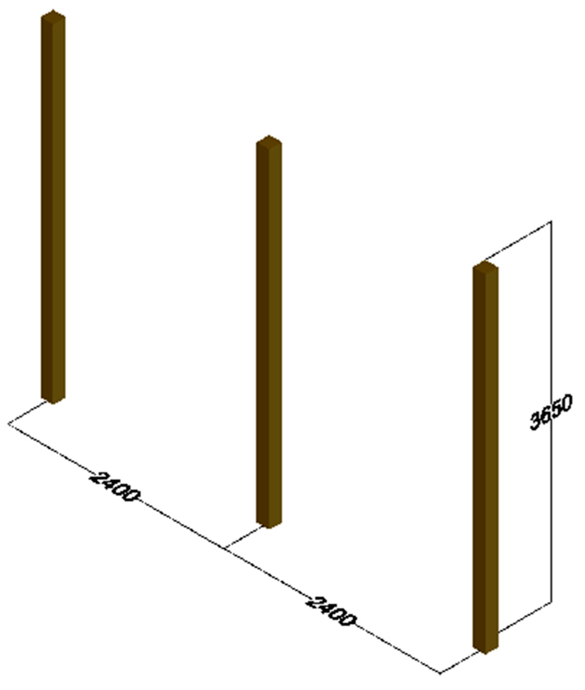
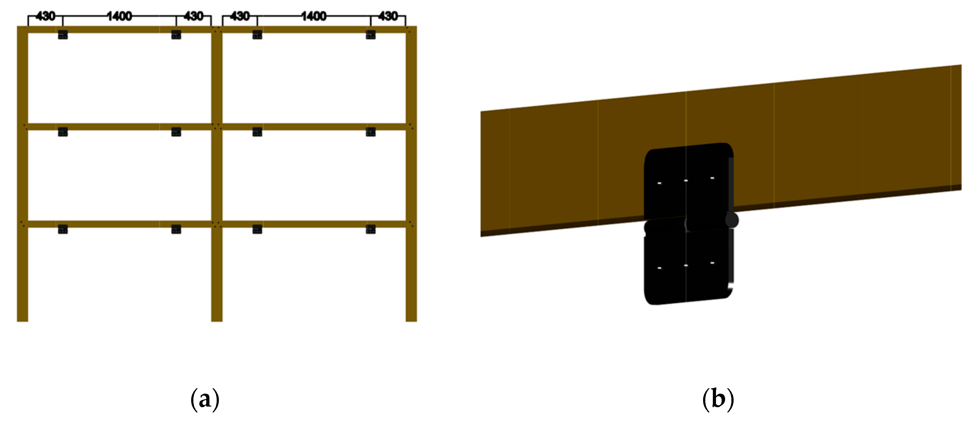
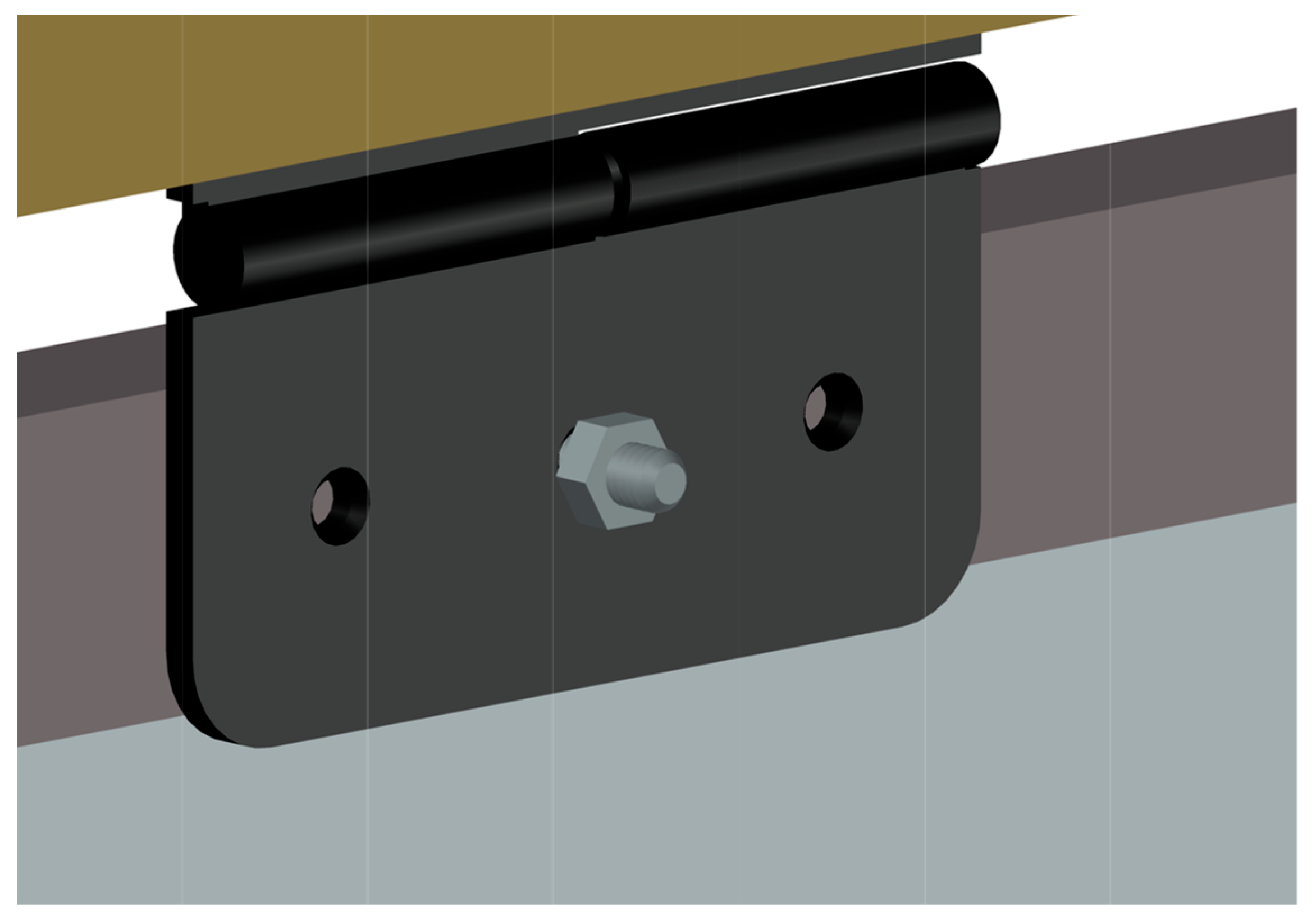
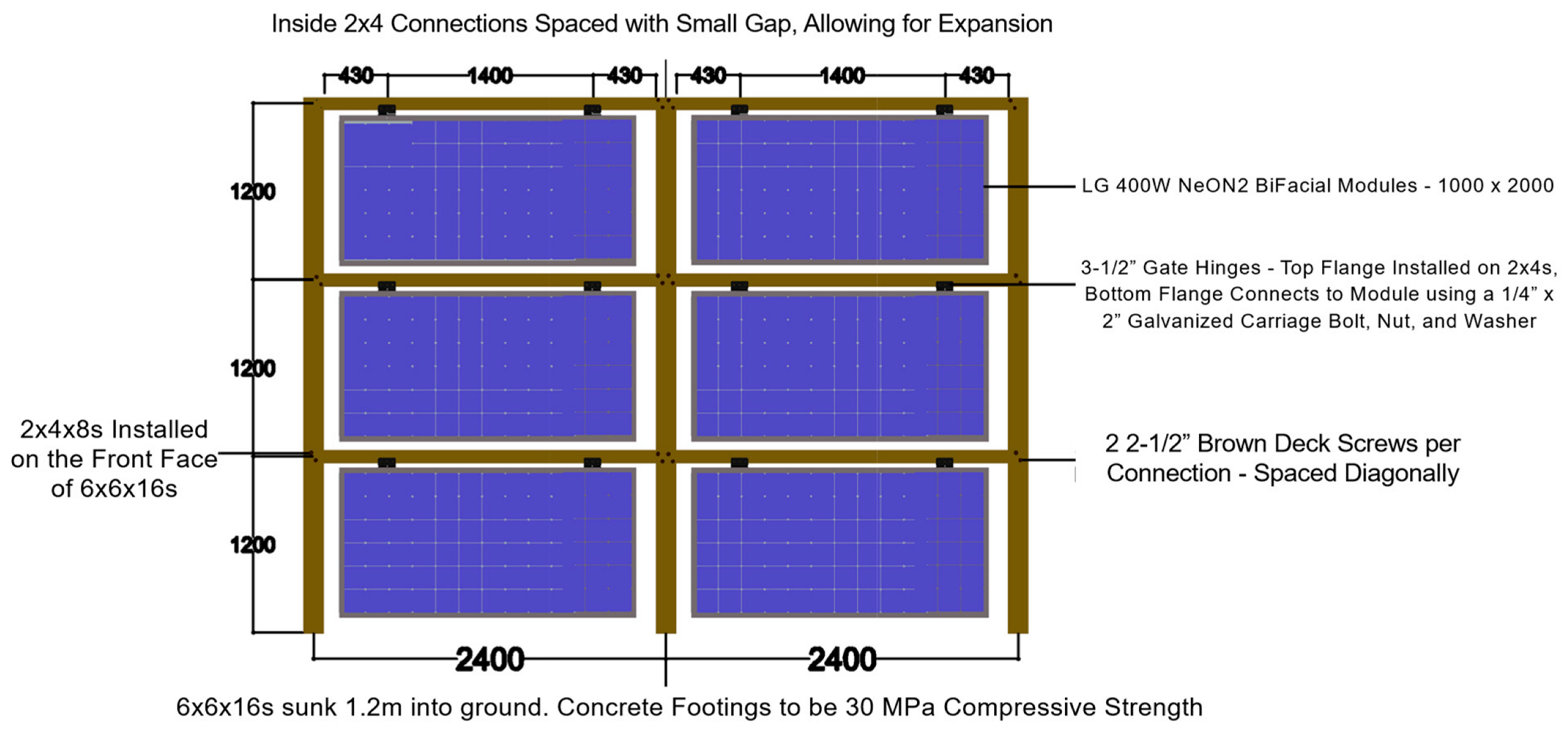
2.1.3. Assembly Instructions

To begin, 6 × 6 × 16 posts must be sunk at least 1.2 m into the ground to prevent frost heaving of any soil type. This is carried out according to the National Building Code of Canada (NBCC) Table 9.12.2.2 [68]. Each post should then be standing 3.65 m above the ground. Each hole should be spaced at 2.4 m, as shown in Figure 1. Holes should be at least 250 mm in diameter. Two bags of 30 kg Quikrete ready-mix concrete can be mixed with water in a wheelbarrow to make footings. Once each hole is filled, the previously removed topsoil can be used to cap the hole. This should be carried out in order to ensure that water runs down the slope away from the footing.
Once the footings have cured and the posts are secured into the ground, 2 × 4 × 8 s can be installed between each post without needing to make any cuts. Each row of 2 × 4 s should be spaced 1.2 m apart, as described in Figure 2a. The 2 × 4 s are installed on the center of the front face of each post with two screws spaced diagonally as shown in Figure 2b. The two 2 × 4 s connected at the interior post’s center should have a small gap between each other to allow room for expansion.
Two 3–½″ outdoor gate hinges are then to be installed along each 2 × 4, as shown in Figure 3a. Install only the top flange to the wood with the screws provided with the hinges. The top flange of the hinge should be installed such that the pin is below the 2 × 4, as shown in Figure 3b. This allows for the full rotation of the bottom flange holding the modules.
Once the hinges are installed, a 1 m × 2 m module can be installed between each row of hinges. Line up each hole of the module with the middle hole of each bottom flange. Replace the hinge screws with ¼″ × 1-1/2″ galvanized carriage bolts to go through the hinge and modules, as shown in Figure 4. The connection can then be secured with a nut and washer on the other side.
The build is complete when all connections are secured as shown in Figure 5. For the end of life, or to move the system, it can then be disassembled in reverse order.

2.2. Energy Performance and Cost Analysis

The energy performance of the proposed system is evaluated using the open source System Advisor Model (SAM) software [69,70]. SAM is preferred as a simulation tool for the proposed PV system energy performance because it is open-source and has been validated against real-world data. It is updated regularly and integrates the latest PV energy calculation methods, such as irradiation models, cell temperature models, inverter models, and different types of losses [71].
The energy performance assessment is conducted for London, Ontario, Canada. In this analysis, the wind speed’s effect on the module is neglected and the modules are assumed to be in a vertical position (90° tilt angle) throughout their lifetime. With this assumption, the system was supposed to have a lower soiling level than a standard fixed tilt system during the simulation, and there was no mutual shading between modules. Additionally, the system’s orientation was considered east–west (90° azimuth angle in London, Ontario) to maximize the incident irradiation on the PV system [72]. The technical performance simulation parameters are shown in Table 2.
The cost analysis relies on the cost per watt. The cost is calculated using 2 = two sections of the proposed vertical wood racks, and then the footing cost is added. Additionally, the energy performance results are used to calculate the levelized cost of electricity (LCOErack) of the racking system. The LCOE is calculated using Equation (1) [77]:
L C O E r a c k   ( $ / k W h ) = N e t   P r e s e n t   V a l u e   o f   t h e   R a c k i n g   ( $ ) N e t   P r e s e n t   V a l u e   o f   P V   E n e r g y   ( k W h )
Here, the cost of the system is used as the net present value of the racking and the energy generated over the system’s lifetime is used as the net present value of energy. The cost per watt and the LCOE of the proposed racking are compared to commercially available vertical metal racking systems. The commercially available racking system cost used in this study is provided by a report on the German market [63]. Additionally, the system cost is compared to other wooden racking systems proposed in the literature for fixed tilt and seasonally adjustable tilt [58,59].

3. Results

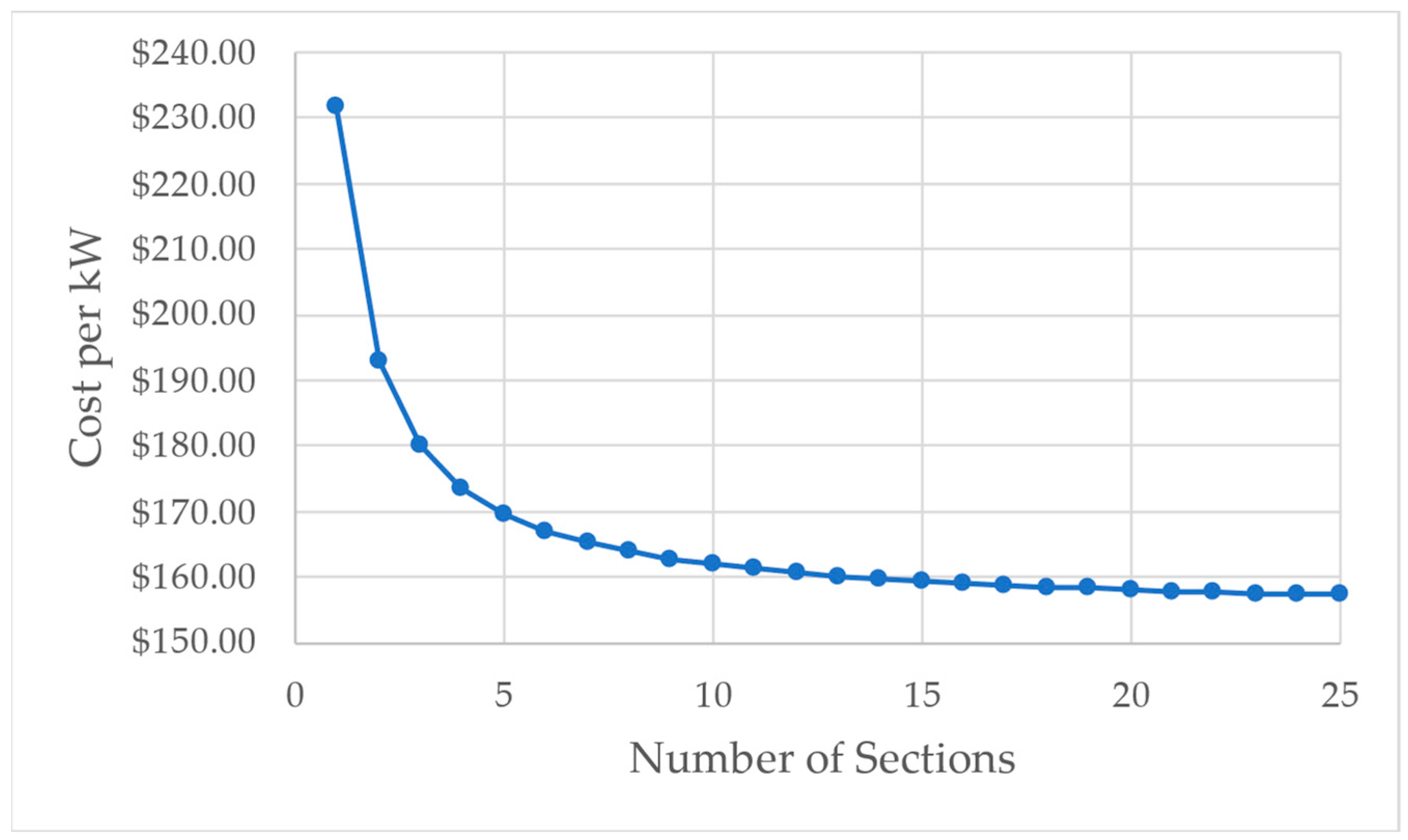
3.1. Cost with Scaling

It should be noted that outside posts carry the load for one half section, while inside posts carry the load for two half sections. Therefore, the more inside posts there are relative to outside posts, the more economically efficient the system becomes. The cost per kW (before footing costs), can be calculated using Equation (2), where S is the number of sections, CostSection is the cost of each section, found in Table 1, Costpost is the cost of each post, and kWSection is the amount of PV power installed on each section.
C k W   ( $ k W ) = C o s t S e c t i o n × S C o s t P o s t × ( S 1 ) k W S e c t i o n × S
Figure 6 graphs this function, which shows the economic benefit of building such a system on a large scale. A system consisting of ten or more sections shows savings of over 30% compared to a system of just one section. Therefore, this system is most desirable to build for large-scale applications. These costs do not consider the additional discount that many hardware stores may honor for purchasing on such a large scale. As the graph tends to infinity, the cost is slightly above CAD 150 per kW (CAD 0.15/W).

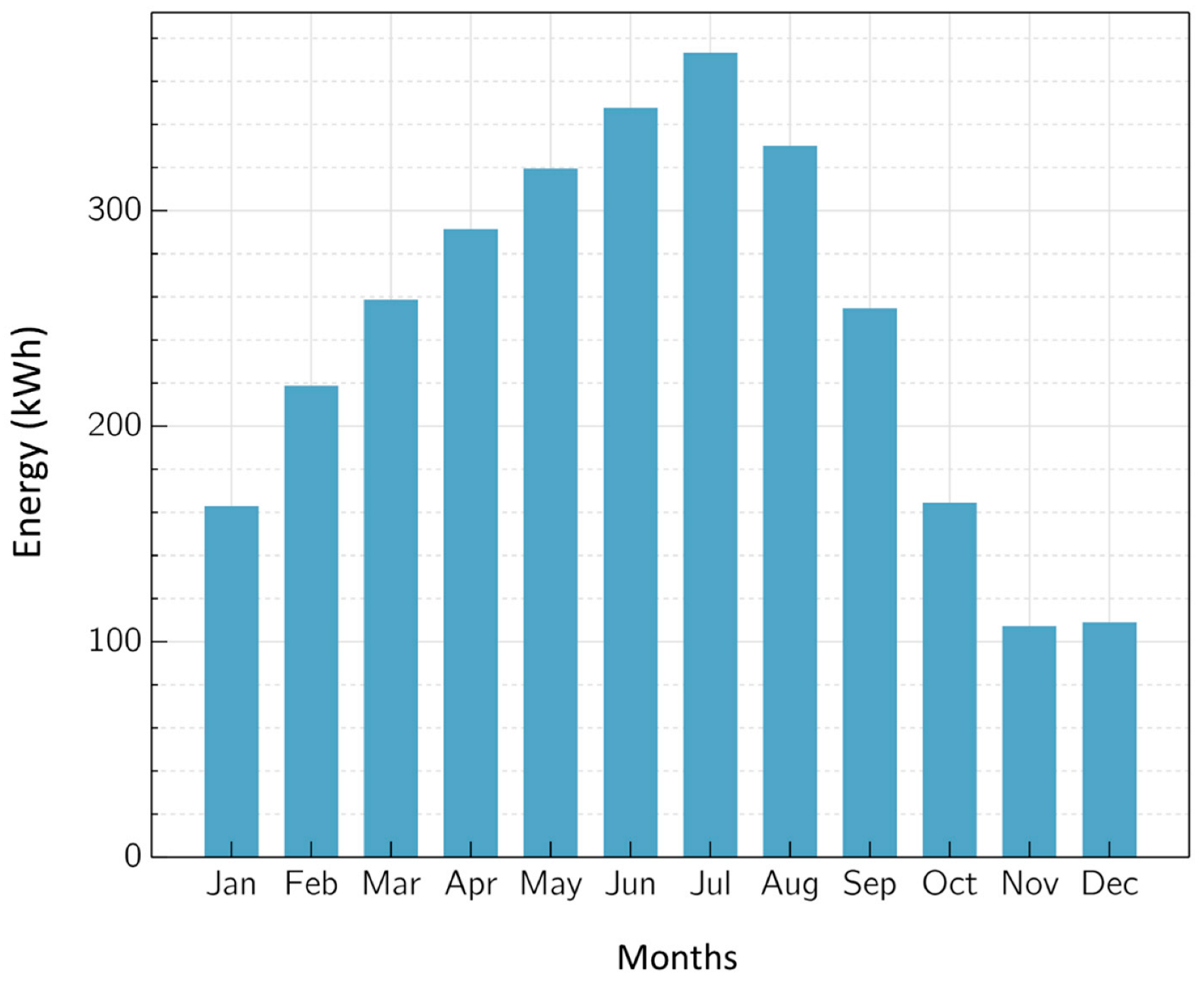
3.2. Energy Performance and Cost Analysis Results

Figure 7 shows the monthly aggregated energy performance of the bifacial vertical tilt PV system during the first operation year. As expected, the system generates more energy during the summer than it does during the winter. The maximum monthly energy production is 373 kWh in July, and the minimum monthly energy production is in November, with 107 kWh. The annual energy generated during the first year is 2938 kWh and the 25-year lifetime energy is 68,940 kWh.
Table 3 shows the cost analysis results of a two-section system made of six PV modules (2.4 kW). The results show the lifetime solar electricity production of the compared systems, as well as the racking cost, the racking LCOE, and the racking cost per watt. The vertical systems generate the least amount of lifetime energy (69 MWh), but are less expensive to install. Fixed-tilt wooden racking and seasonal-tilt wooden racking have a higher racking cost, but they also have a higher energy production than the two vertical systems. Even though the LCOEs of fixed-tilt and seasonal-tilt racks (~CAD 0.01/kWh) are close to the commercial metal vertical racking, the proposed vertical wooden system has an overall lower LCOE (~CAD 0.007/kWh). Additionally, the proposed system has the lowest cost per rack (~CAD 0.21/W). CAD 0.21/W is 22%, 34%, and 38% lower than the commercial metal vertical racking, the wood fixed tilt racking, and the wood seasonal tilt racking costs, respectively. As a result, the proposed vertical free-swinging wood racking appears to be the least expensive racking system in terms of cost per watt to date.

4. Discussion

4.1. Limitations and Future Work

The results shown for both the mechanical analysis (that the system should meet/exceed all Canadian building standards) as well as the base economics make this open-source vertical racking design promising for agrivoltaic applications as well as the potential to be used in other vertical applications. Some examples include privacy screens, fences [54,79,80], and highway sound barriers [81,82,83,84]. There are several areas of important future work. First, this was a theoretical design study and future work is needed to experimentally test the systems in the field and catalog for what farming equipment and crops the systems are appropriate/inappropriate in real-world conditions. Conventional agrivoltaics studies need to be run on this racking system with a wide range of field crops. In particular, the agricultural community would benefit from the knowledge of the impact on crops as a function of the distance from the vertical arrays (e.g., if they function as windbreaks with their concomitant benefits [85,86,87,88]). This knowledge will also assist in choosing optimum spacing between rows, while keeping in mind the energy values and farm equipment spacing requirements.
The second main limitation of this study involves the assumptions used for the modeling. It is well-established that spectral albedo has a large impact on PV performance [89,90]. The spectral albedo is particularly important for bifacial PV modules, as proposed in this work [91,92]. In this study, none of these considerations were included in the simulations. Future work could install an experimental vertical rack and utilize an open-source spectral albedometer [93] to quantify the potential positive impact different types of field crops would have on this system. Finally, a limitation of this study was assuming that the system would always have a vertical position. This is the case in low-wind velocity areas. Other areas, however, that experience increased wind velocities would have the PV at non-vertical tilt angles during operation. In general, this would be expected to increase the performance, so the assumptions used here should be considered conservative and likely to underestimate the total yield. Future work could propose a SAM extension to account for the velocity-dependent tilt angle of this system, as well as providing guidance for which side should be the ‘front’ for bifacial modules in a given location, given the mismatch between the front and the back [94,95,96].
Regarding vertical racks for agrivoltaics with rows spaced further than conventional solar farms, it is expected that the capacity factor would be increased due to freer air flow, resulting in lower operating temperatures as well as radically reduced row-to-row shading. Contrariwise, a small increase in the DC losses would be expected because of longer cable lengths. Further work is needed to determine the cost benefit of changing the energy density for this type of vertical agrivoltaics systems compared to conventional solar farms. These advantages can be added to the capital costs found in this study. Finally, some social science future work is necessary to evaluate the potential for broader acceptance, and thus more total land area will become available with this approach.

4.2. Wood Price Sensitivity

The economics of this vertical wood-based racking system are particularly promising in North America, where it was designed. It should be pointed out, however, that the economics are very sensitive to the commercial price of lumber. This price is known to be volatile, as shown in the sensitivity analysis in the [36] design.
In addition to the global price fluctuations, the BOM costs will also be dependent on the prices at the local sources of wood, whether it is available at all, and, if imported, the taxes and import duties.
Given the variance in wood costs, future work can also investigate designing and building a vertical PV rack made from other materials, using these designs as a baseline (e.g., waste plastic lumbar, metal, etc.).

5. Conclusions

This open-source vertical wood-based solar PV rack is (i) made from locally accessible (domestic) renewable and sustainable materials, (ii) can be made with hand tools by average farmers on their farms, (iii) has a lifetime of 25 years to match those of PV module warranties, (iv) is structurally sound, following Canadian building codes to withstand high speeds and heavy snow loads, (v) has a relatively low capital cost compared to commercially available offerings and (vi) is shared using a free and open source license so that individuals or companies can make it for themselves or others. Others are particularly encouraged to make versions to offer people in their local markets. This study provided an open-source wood-based solar PV racking design that successfully overcame the cost challenge of proprietary vertical commercial racks. The results showed that the capital cost of the racking system is less expensive than the commercial equivalent, and all of the previous wood-based rack designs. The racking cost is CAD 0.21, even at the single system scale using retail costs of materials. The racking LCOE is 77% of the cost of an equivalent commercial racking system. The open-source design consists of a hinge mechanism, which is the first of its kind.

6. OSHWA Certification in Place of Patents

Upon acceptance, the designs will be OSHWA certified and the number will be added here.

Author Contributions

Conceptualization, J.M.P.; supervision, J.M.P.; funding acquisition, J.M.P.; methodology, N.V. and K.S.H.; software, K.S.H.; validation, N.V. and K.S.H.; formal analysis, J.M.P., N.V. and K.S.H.; investigation, N.V. and K.S.H.; visualization, N.V. and K.S.H.; resources, J.M.P.; data curation, N.V. and K.S.H.; writing—original draft preparation J.M.P., N.V. and K.S.H.; writing—review and editing, J.M.P., N.V. and K.S.H. All authors have read and agreed to the published version of the manuscript.

Funding

This research was funded by the Natural Sciences and Engineering Research Council of Canada (NSERC) and the Thompson Endowment.

Institutional Review Board Statement

Not applicable.

Informed Consent Statement

Not applicable.

Data Availability Statement

Data will be made available upon request.

Conflicts of Interest

The authors declare no conflict of interest. The funders had no role in the design of the study; in the collection, analyses, or interpretation of data; in the writing of the manuscript, or in the decision to publish the results.

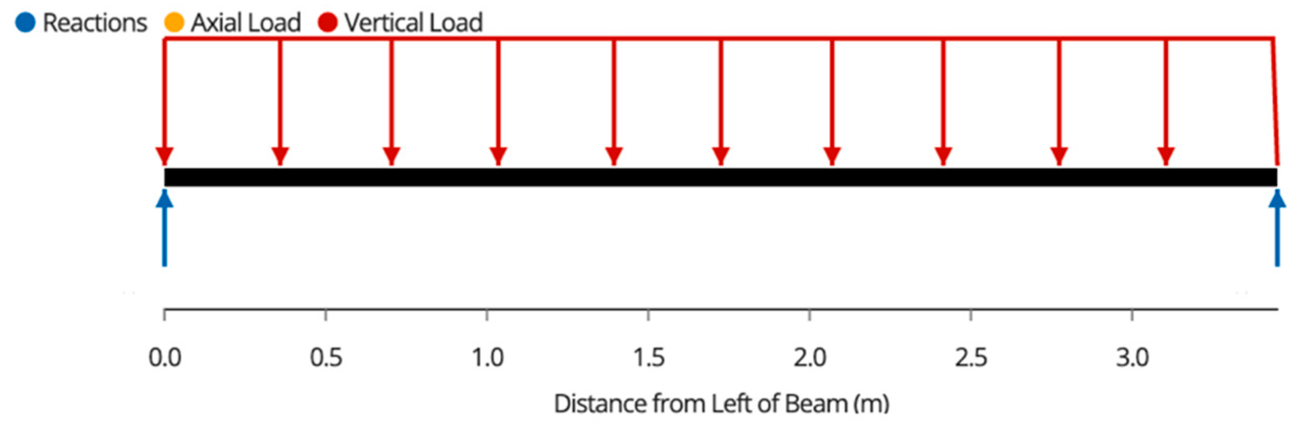
Appendix A. Specified Loads

Vertical modules supported by joists and posts can best be represented as a simple sign structure, and thus it is best practice to consult MTO’s Sign Support Manual [97] and ASCE 7–16 Section 29.3 Design Wind Loads for Solid Signs [98] to obtain the design load for a given location.
The design wind load can be calculated using Equation (A1).
D e s i g n   W i n d   L o a d = 1.4 q K z K z t K d K e G C f
As per the NBCC 4.1.3.2 [68], a safety factor of 1.4 must be applied to specified wind loads to reduce the probability of failure.
The velocity pressure, q, will be taken as 455 Pa for London, Ontario, as per Table A2.9(b) of MTO’s Sign Support Manual [97].
Kz is the velocity pressure exposure coefficient, which can be taken as 0.85 for structures less than 15 feet tall in open terrain.
Kzt is the topographic factor, which can be taken as 1.00 for structures not placed near large hills or escarpments.
Kd is the directionality factor, which can be taken as 0.85 if the structure serves as an open frame.
Ke is the ground elevation factor, which can be taken as 1.00 for all elevations as a conservative assumption.
G is the gust-effect factor, which can be taken as 0.85 for rigid structures not subject to high-rise dynamic oscillation.
Finally, Cf is the force coefficient, and experimental testing suggests that 1.30 can be taken for open space frame structures [99].
Inputting all the factors into Equation (A1) produces a design wind load of 0.51 kPa.
The value of each coefficient is the same for all locations, with the exception of the velocity pressure, q,. If this pressure is not readily tabulated, it can be calculated using the wind pressure Equation (A2) shown below:
q = 1 2 ρ V 2
where ρ is the density of air taken as 1.225 [68], and V is the 1-in-25-year wind speed.
The velocity pressure of 455 Pa satisfies the wind speed design requirements for over 95% of Ontario [97], and over 85% of Canada (including territories and coasts) [68].

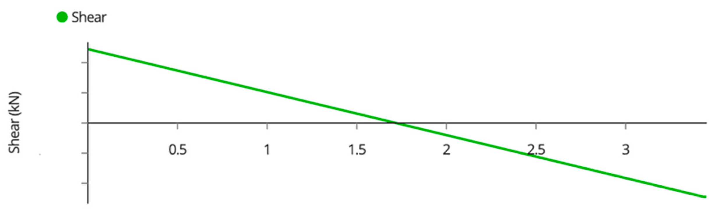
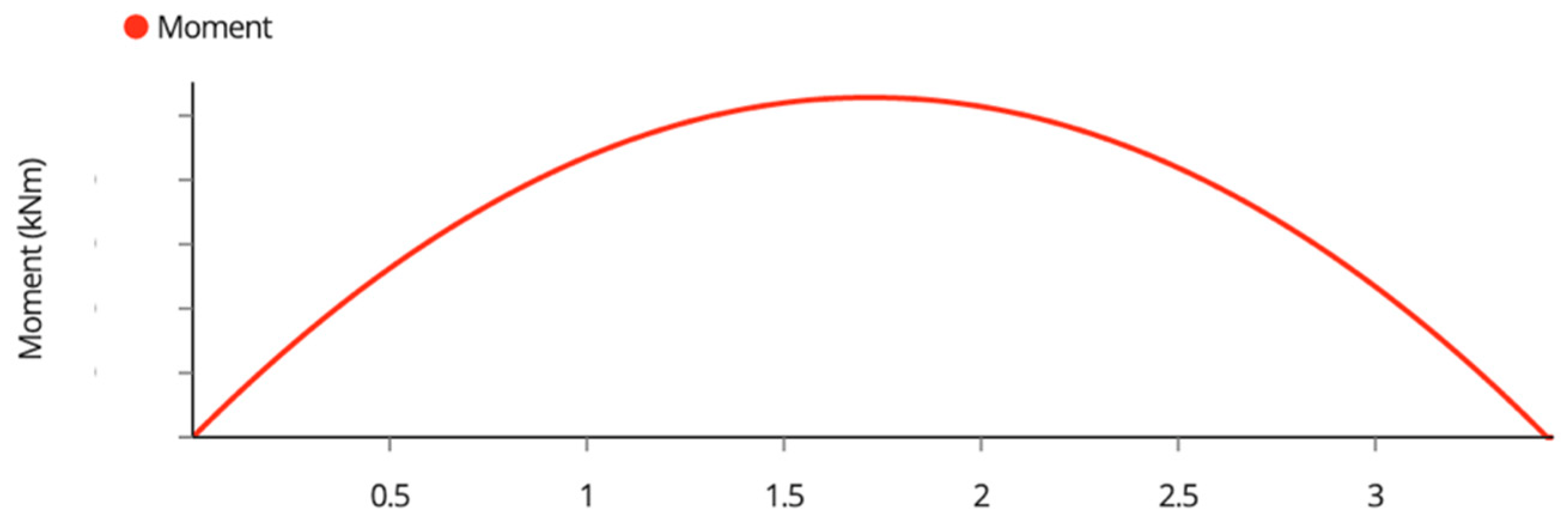
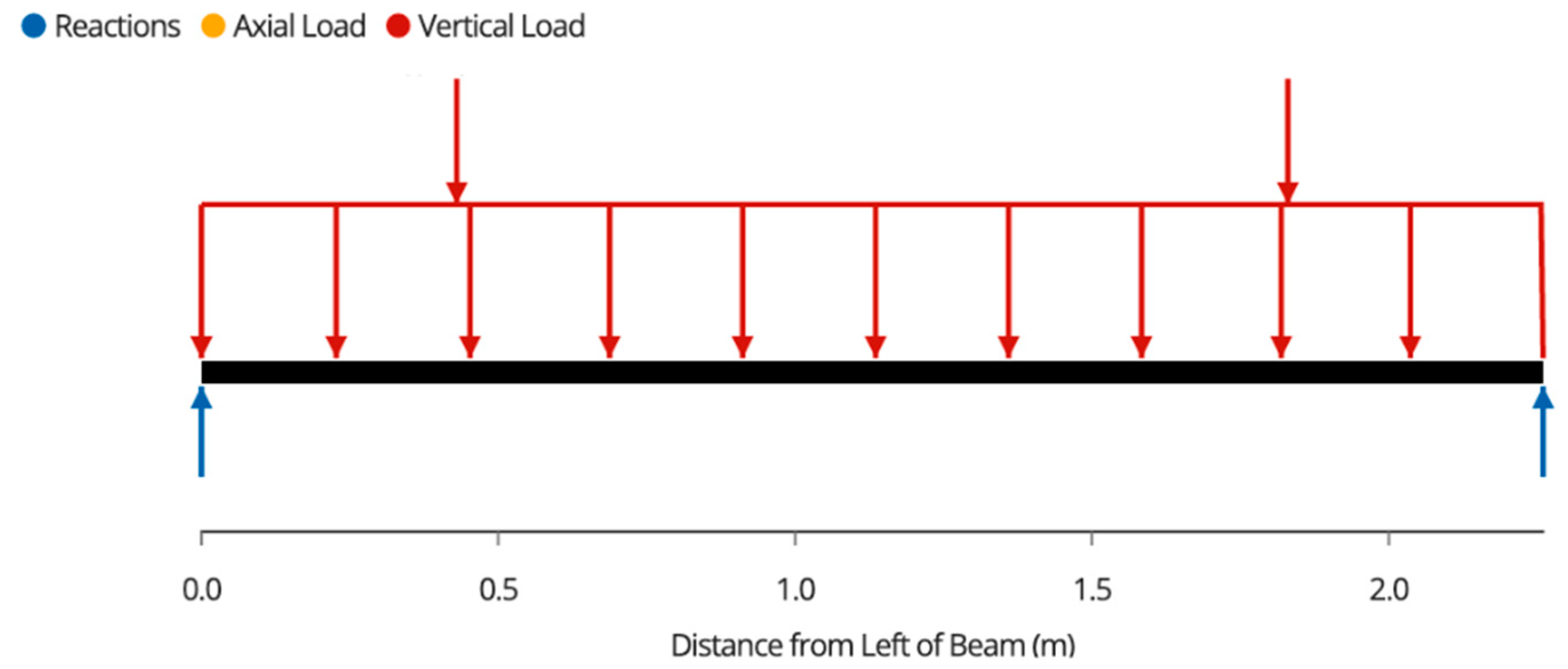
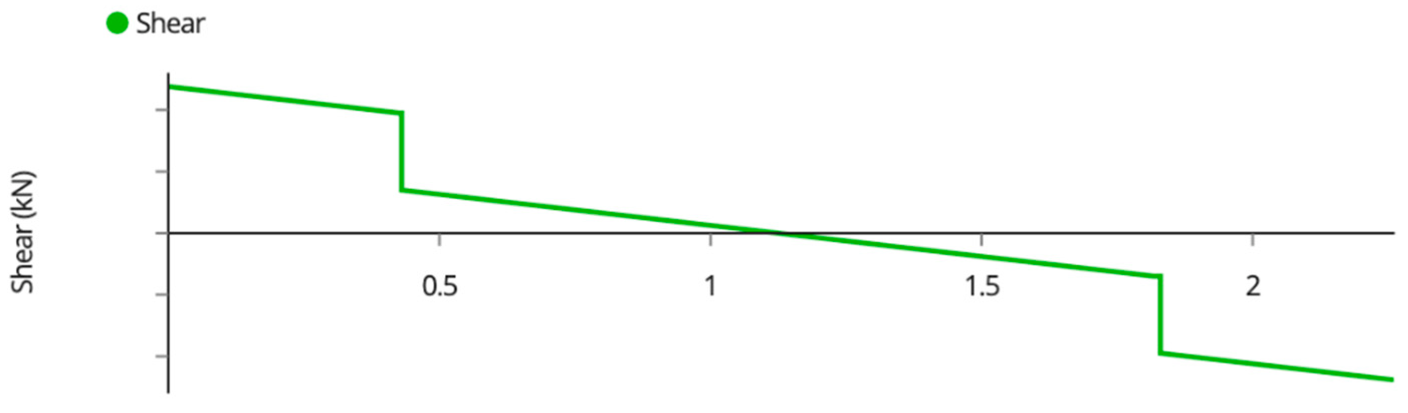
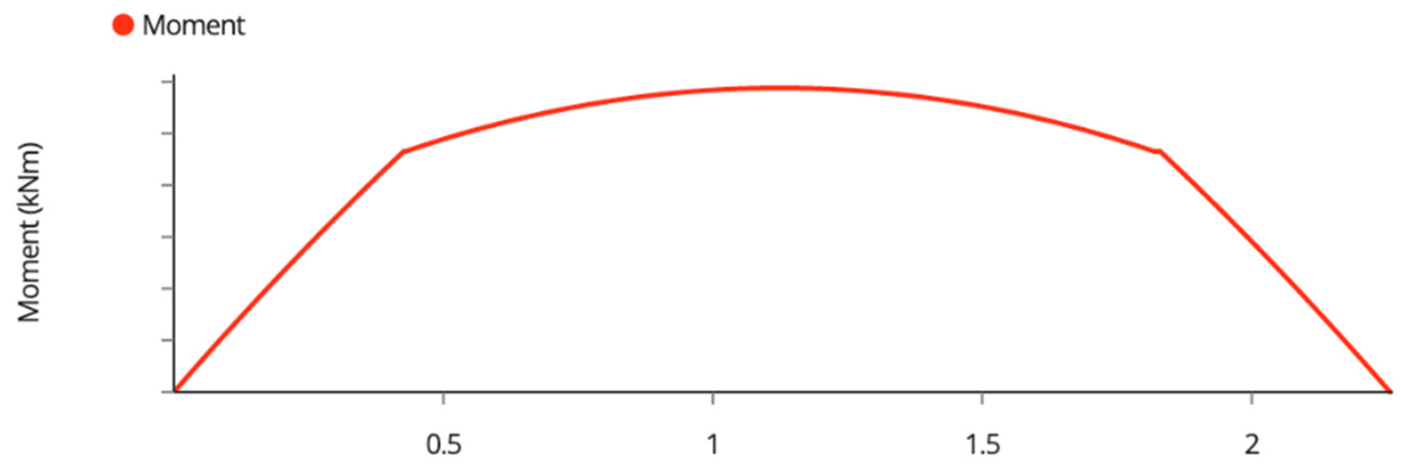
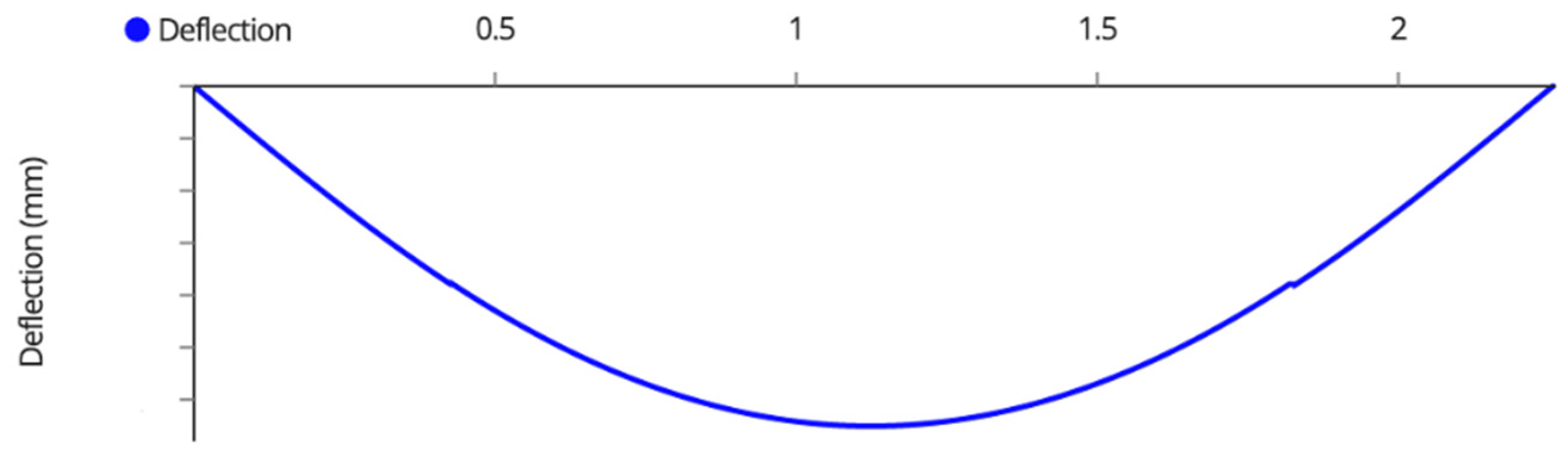
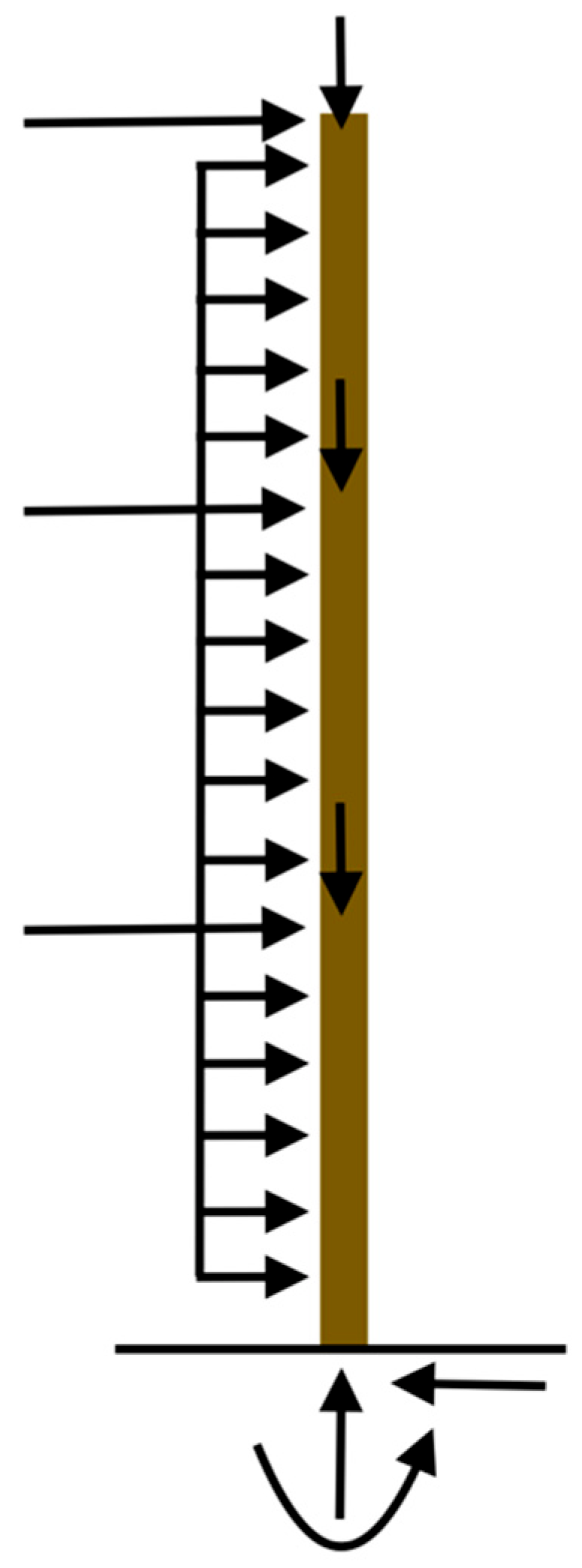
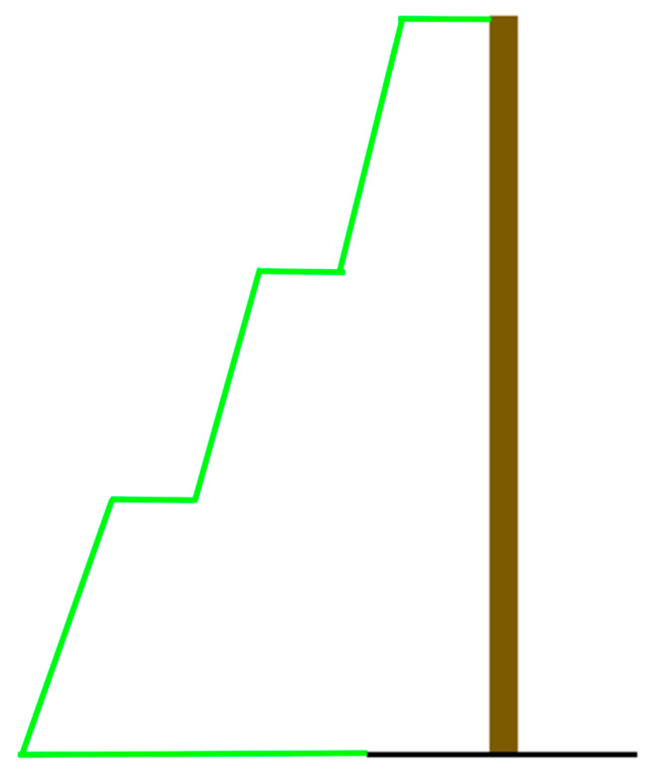
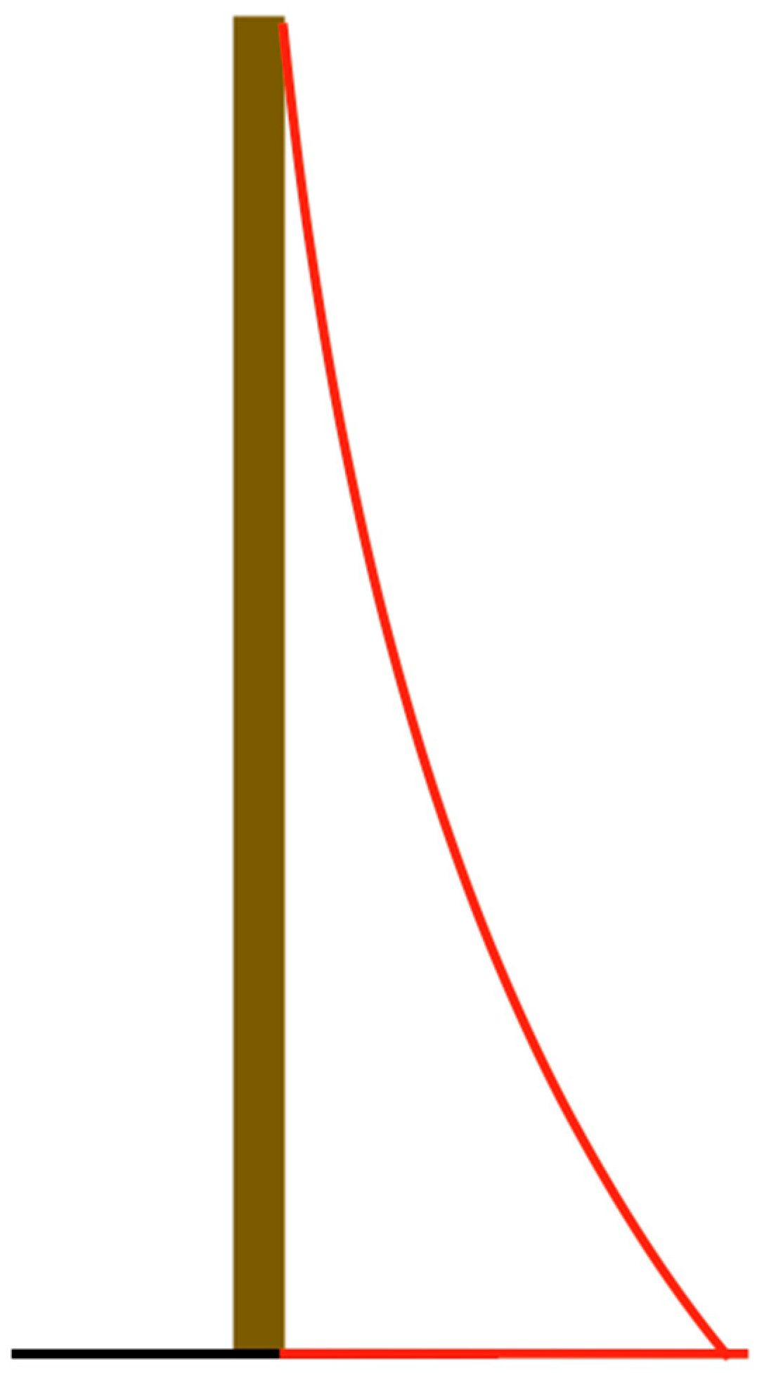
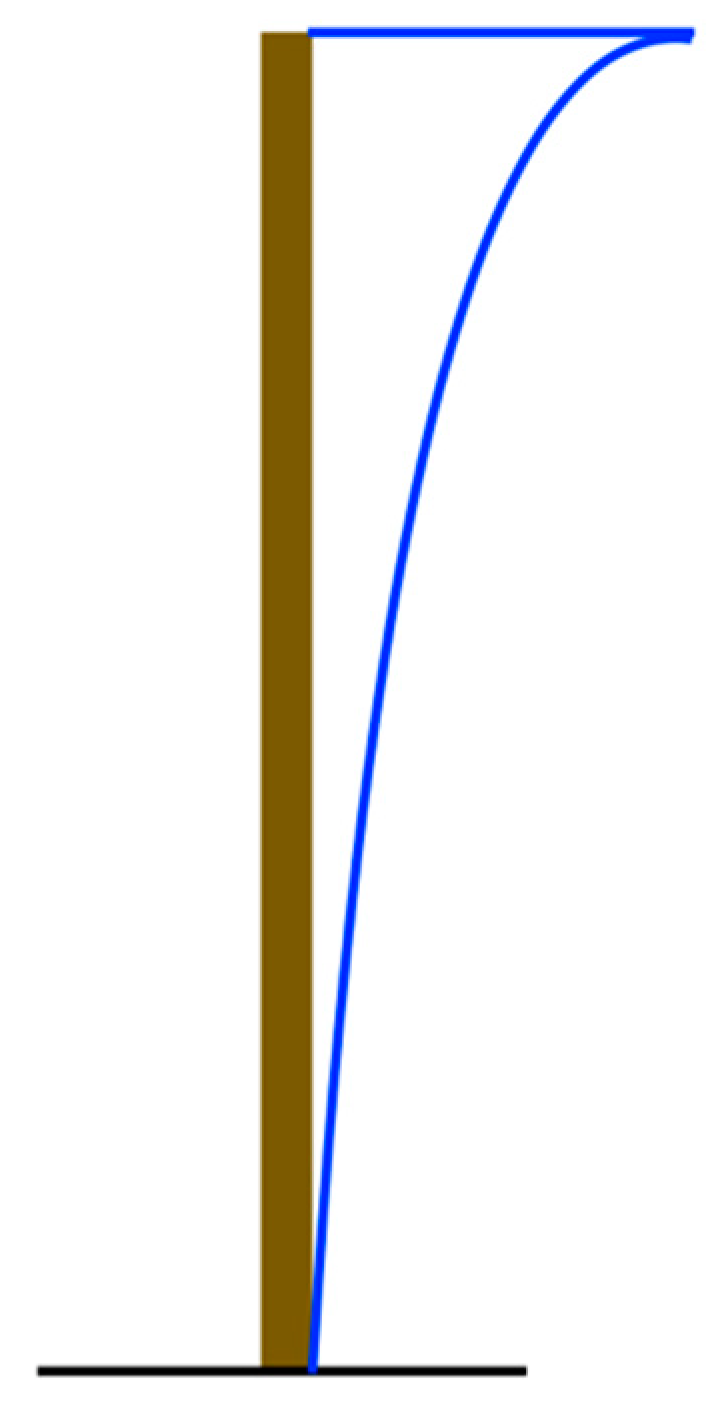
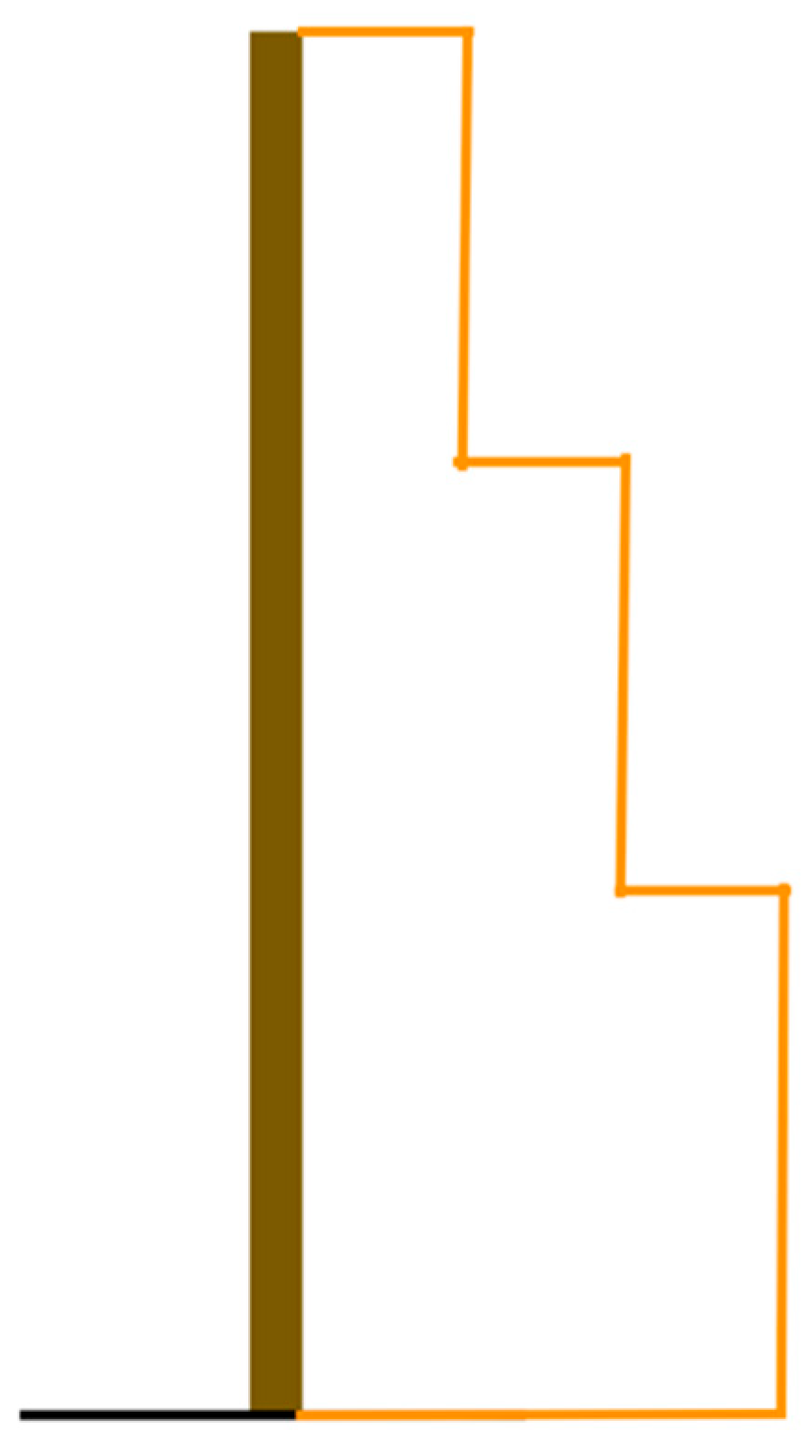
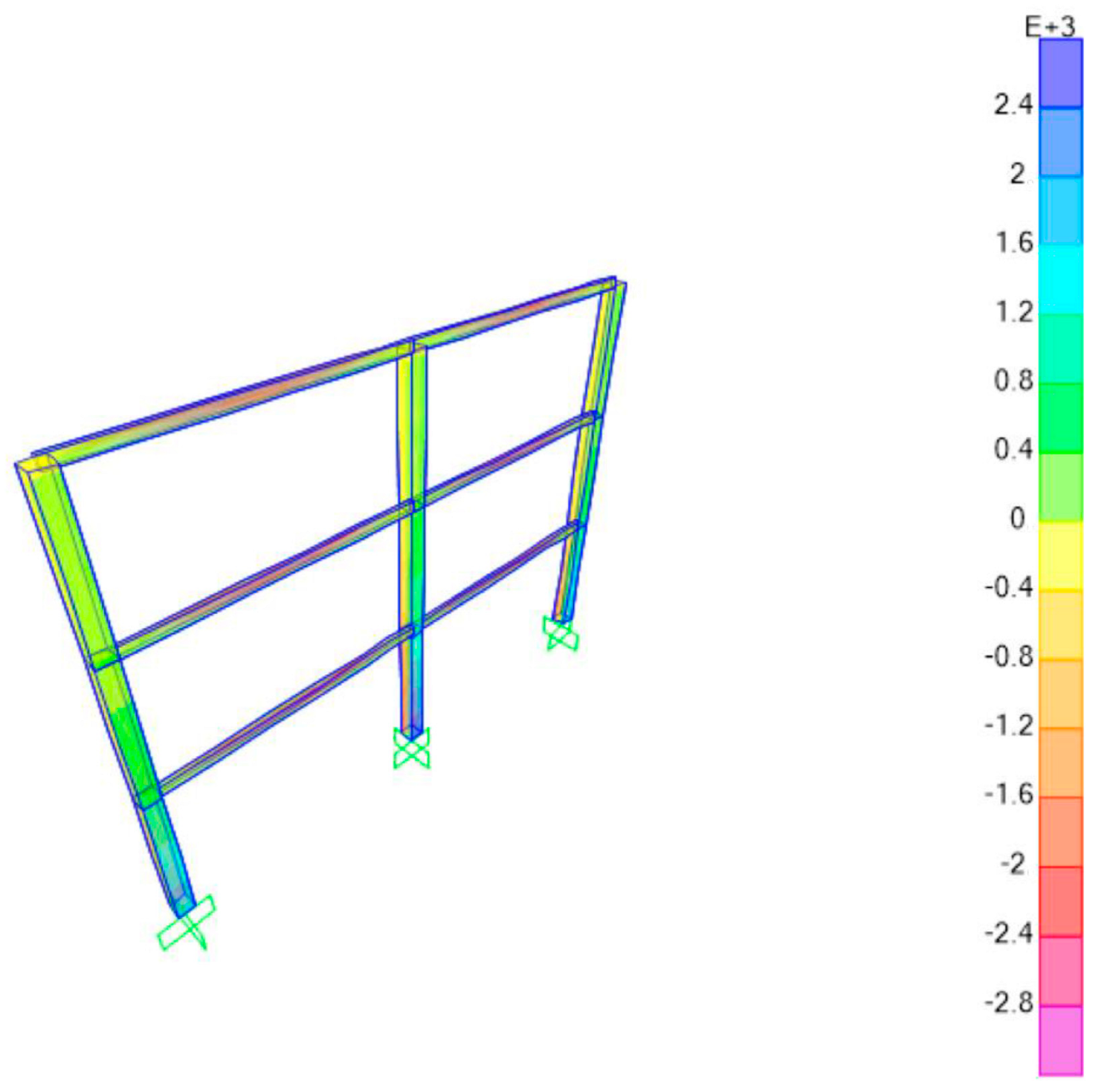
Appendix B. Vertical System Structural Analysis

Since the modules are connected to the 2 × 4 s via hinges, the wind force will rotate the modules rather than strain them, and thus there is no static load to be applied to the modules. Both the lateral wind loads and downwards gravity loads must be analyzed, and the combination of these loads using a stress analysis must be used. Throughout this process, the structural capacities of lumber outlined in Vandewetering et al. [58], which summarizes the design requirements of the National Design Specification for Wood Construction [67], shall not be exceeded.
First, the wind load will attack the 2 × 4 s upon the weak axis. Each 2 × 4 will serve as a simply supported beam carrying a uniform distributed wind load. The magnitude of the distributed load is calculated using Equation (A2):
w = D e s i g n   W i n d   L o a d M e m b e r   W i d t h
For 2 × 4 s, the width being attacked by wind is 89 mm, or 0.089 m. The free body diagram of each 2 × 4 as shown in Figure A1 below.
Figure A1. The 2 × 4 Wind Load Free-Body Diagram.
Designs 07 00034 g0a1
The shear force diagram of each 2 × 4 is seen as in Figure A2.
Figure A2. The 2 × 4 Wind Load Shear Force Diagram.
Designs 07 00034 g0a2
The maximum shear force occurs at the supports, which can be calculated using Equation (A3).
V m a x 2 × 4 W i n d = w L 2
The bending moment diagram of each 2 × 4 is seen as in Figure A3.
Figure A3. The 2 × 4 Wind Load Bending Moment Diagram.
Designs 07 00034 g0a3
The maximum bending moment occurs at midspan. The maximum bending moment can be calculated by Equation (A5).
M m a x 2 × 4 W i n d = w L 2 8
The deflection diagram throughout each 2 × 4 is seen as in Figure A4.
Figure A4. The 2 × 4 Wind Load Deflection Diagram.
Designs 07 00034 g0a4
The maximum deflection occurs at midspan and can be calculated using Equation (A6).
Δ m a x 2 × 4 W i n d = 5 w L 4 384 E I
On the strong axis of each 2 × 4, the self-weight and the weight of two modules must be carried. This loading can be modelled with a uniform distributed self-weight, and the two point loads from the weight of the modules are as shown in Figure A5.
Figure A5. The 2 × 4 Weight Free Body Diagram.
Designs 07 00034 g0a5
The shear force diagram is shown in Figure A6.
Figure A6. The 2 × 4 Weight Shear Force Diagram.
Designs 07 00034 g0a6
The maximum shear force can be calculated using Equation (A7).
V m a x 2 × 4 W e i g h t = 1.25 ( S i n g l e   M o d u l e   W e i g h t + o w 2 × 6 × L 2 )
The bending moment diagram is shown in Figure A7.
Figure A7. The 2 × 4 Weight Bending Moment Diagram.
Designs 07 00034 g0a7
The maximum moment occurs at midspan, and is calculated using Equation (A8).
V m a x 2 × 4 W e i g h t = 1.25 ( S i n g l e   M o d u l e   W e i g h t 2 x + o w 2 × 6 × L 2 8 )
where 1.25 is taken as the factor of safety for dead loads [68].
The deflection diagram is shown in Figure A8.
Figure A8. The 2 × 4 Weight Deflection Diagram.
Designs 07 00034 g0a8
Additionally, the maximum deflection is calculated using Equation (A9).
Δ m a x 2 × 4 W e i g h t = 5 o w 2 × 6 L 4 384 E I + P o i n t   L o a d x ( L x ) 6 E I L ( L 2 4 + x 2 L 2 )
Since the 2 × 4 s serve as beams carrying biaxial bending, the combination of gravity and wind stresses must be less than the maximum bending capacity, as described in Equation (A10).
M f W e i g h t + M f W i n d f b *
The bending stress due to gravity can be calculated using Equation (A11).
M f W e i g h t = 6 M m a x 2 × 4 W e i g h t b h 2
The bending stress due to wind can be calculated using Equation (A12).
M f W i n d = 6 M m a x 2 × 4 W i n d h b 2
The load is then transferred to the 6 × 6 posts, which can be idealized as a cantilever beam column carrying a uniform distributed wind load, a series of point loads from the 2 × 4 wind loads, the weight of the system, and the post’s own weight. The uniform distributed load, w, is calculated the same way as the 2 × 4 s, but now with a member width of 140 mm, or 0.14 m. The magnitudes of the point loads are equal to the reactions from each 2 × 4, which conveniently equals the shear force of each 2 × 4 carried, Vmax2×4. It should be noted that each inside post carries a 2 × 4 from two sections, so the magnitude of each point load is twice the magnitude of the outside posts. The free body diagram of each post is described in Figure A9.
Figure A9. The 6 × 6 Free-Body Diagram.
Designs 07 00034 g0a9
The shear force diagram is seen in Figure A10.
Figure A10. The 6 × 6 Shear Force Diagram.
Designs 07 00034 g0a10
The maximum shear force occurs at the footing, and can be calculated using Equation (A13).
V m a x 6 × 6 = V m a x 2 × 6 W i n d + w L
The bending moment diagram of each post is shown in Figure A11.
Figure A11. The 6 × 6 Bending Moment Diagram.
Designs 07 00034 g0a11
The maximum bending moment occurs at the footing, and can be calculated using Equation (A13).
M m a x 6 × 6 = ( V m a x 2 × 6 W i n d x ) + w L 2 2
where x is the distance from the footing to each of the 2 × 4 reactions.
The deflection diagram is shown as in Figure A12.
Figure A12. The 6 × 6 Deflection Diagram.
Designs 07 00034 g0a12
The maximum deflection occurs at the top of the post, and can be calculated using Equation (A15).
Δ m a x 6 × 6 = V m a x 2 × 4 ( x ) 2 6 E I ( 3 L x ) + w L 4 8 E I
The compression load throughout the post varies as shown in Figure A13.
Figure A13. The 6 × 6 Compression Diagram.
Designs 07 00034 g0a13
The maximum compression occurs at the base, and has a max value given by Equation (A16).
C m a x = 1.25 o w 6 × 6 + V m a x 2 × 6 W e i g h t
The combination of axial compression and bending cause requires a combined loading stress analysis to ensure the fibers in compression do not exceed the wood’s capacity. The load combination limit is described in Equation (A17).
C m a x f c * + M f W i n d f b * 1.00
The resulting shear, moments, deflections and stresses for a design load of 0.51 kPa have been summarized in Table A1.
Table A1. Forces, deflections and stresses of structural members.
LumberShear [kN]Moment [kNm]Deflection [mm]Compression [kN]Stress [MPa]
2 × 4 Wind0.050.0322.24N/A1.47
2 × 4 Weight0.130.072.92N/A1.56
Outside 6 × 60.410.830.020.391.93
Inside 6 × 60.581.260.010.792.80
The system can also be analyzed using FEA software such as SAP2000 to ensure that the wood does not exceed the maximum allowable stress. The stress contour of a two-section model is shown in Figure A14. The percentage difference between the analytical hand calculation approach and the FEA approach is less than 2.5%.
Figure A14. Stress contour of a two-section system, where the max stress of 2.81 MPa occurs at the base of the interior post.
Designs 07 00034 g0a14

References

  1. CSIRO GenCost: Annual Electricity Cost Estimates for Australia. Available online: https://www.csiro.au/en/research/technology-space/energy/energy-data-modelling/gencost-2021-22 (accessed on 10 January 2023).
  2. Pearce, J.; Lau, A. Net Energy Analysis for Sustainable Energy Production from Silicon Based Solar Cells. In Proceedings of the Solar Energy; ASMEDC: Reno, NV, USA, 2002; pp. 181–186. [Google Scholar]
  3. Bhandari, K.P.; Collier, J.M.; Ellingson, R.J.; Apul, D.S. Energy Payback Time (EPBT) and Energy Return on Energy Invested (EROI) of Solar Photovoltaic Systems: A Systematic Review and Meta-Analysis. Renew. Sustain. Energy Rev. 2015, 47, 133–141. [Google Scholar] [CrossRef]
  4. Denholm, P.; Margolis, R.M. Land-Use Requirements and the per-Capita Solar Footprint for Photovoltaic Generation in the United States. Energy Policy 2008, 36, 3531–3543. [Google Scholar] [CrossRef]
  5. Wüstenhagen, R.; Wolsink, M.; Bürer, M.J. Social Acceptance of Renewable Energy Innovation: An Introduction to the Concept. Energy Policy 2007, 35, 2683–2691. [Google Scholar] [CrossRef] [Green Version]
  6. Batel, S.; Devine-Wright, P.; Tangeland, T. Social Acceptance of Low Carbon Energy and Associated Infrastructures: A Critical Discussion. Energy Policy 2013, 58, 1–5. [Google Scholar] [CrossRef]
  7. Calvert, K.; Mabee, W. More Solar Farms or More Bioenergy Crops? Mapping and Assessing Potential Land-Use Conflicts among Renewable Energy Technologies in Eastern Ontario, Canada. Appl. Geogr. 2015, 56, 209–221. [Google Scholar] [CrossRef]
  8. Calvert, K.; Pearce, J.M.; Mabee, W.E. Toward Renewable Energy Geo-Information Infrastructures: Applications of GIScience and Remote Sensing That Build Institutional Capacity. Renew. Sustain. Energy Rev. 2013, 18, 416–429. [Google Scholar] [CrossRef] [Green Version]
  9. Groesbeck, J.G.; Pearce, J.M. Coal with Carbon Capture and Sequestration Is Not as Land Use Efficient as Solar Photovoltaic Technology for Climate Neutral Electricity Production. Sci. Rep. 2018, 8, 13476. [Google Scholar] [CrossRef] [Green Version]
  10. Runge, C.F.; Senauer, B. How biofuels could starve the poor. Foreign Aff. 2007, 86, 41. [Google Scholar]
  11. Tenenbaum, D.J. Food vs. Fuel: Diversion of Crops Could Cause More Hunger. Environ. Health Perspect. 2008, 116, A254–A257. [Google Scholar] [CrossRef] [Green Version]
  12. Tomei, J.; Helliwell, R. Food versus Fuel? Going beyond Biofuels. Land Use Policy 2016, 56, 320–326. [Google Scholar] [CrossRef]
  13. Sovacool, B. Exploring and Contextualizing Public Opposition to Renewable Electricity in the United States. Sustainability 2009, 1, 702–721. [Google Scholar] [CrossRef] [Green Version]
  14. Sovacool, B.K.; Lakshmi Ratan, P. Conceptualizing the Acceptance of Wind and Solar Electricity. Renew. Sustain. Energy Rev. 2012, 16, 5268–5279. [Google Scholar] [CrossRef]
  15. Dias, L.; Gouveia, J.P.; Lourenço, P.; Seixas, J. Interplay between the Potential of Photovoltaic Systems and Agricultural Land Use. Land Use Policy 2019, 81, 725–735. [Google Scholar] [CrossRef]
  16. Dupraz, C.; Marrou, H.; Talbot, G.; Dufour, L.; Nogier, A.; Ferard, Y. Combining Solar Photovoltaic Panels and Food Crops for Optimising Land Use: Towards New Agrivoltaic Schemes. Renew. Energy 2011, 36, 2725–2732. [Google Scholar] [CrossRef]
  17. Mavani, D.D.; Chauhan, P.M.; Joshi, V.P. Beauty of Agrivoltaic System Regarding Double Utilization of Same Piece of Land for Generation of Electricity & Food Production. Int. J. Sci. Eng. Res. V 2019, 10, 118. [Google Scholar]
  18. Pearce, J.M. Photovoltaics—A Path to Sustainable Futures. Futures 2002, 34, 663–674. [Google Scholar] [CrossRef]
  19. Fthenakis, V.M.; Betita, R.; Shields, M.; Vinje, R.; Blunden, J. Life Cycle Analysis of High-Performance Monocrystalline Silicon Photovoltaic Systems: Energy Payback Times and Net Energy Production Value. In Proceedings of the 27th European Photovoltaic Solar Energy Conference and Exhibition, Frankfurt, Germany, 24 September 2012; pp. 4667–4672. [Google Scholar] [CrossRef]
  20. Marrou, H.; Wery, J.; Dufour, L.; Dupraz, C. Productivity and Radiation Use Efficiency of Lettuces Grown in the Partial Shade of Photovoltaic Panels. Eur. J. Agron. 2013, 44, 54–66. [Google Scholar] [CrossRef]
  21. Valle, B.; Simonneau, T.; Sourd, F.; Pechier, P.; Hamard, P.; Frisson, T.; Ryckewaert, M.; Christophe, A. Increasing the Total Productivity of a Land by Combining Mobile Photovoltaic Panels and Food Crops. Appl. Energy 2017, 206, 1495–1507. [Google Scholar] [CrossRef]
  22. Barron-Gafford, G.A.; Pavao-Zuckerman, M.A.; Minor, R.L.; Sutter, L.F.; Barnett-Moreno, I.; Blackett, D.T.; Thompson, M.; Dimond, K.; Gerlak, A.K.; Nabhan, G.P.; et al. Agrivoltaics Provide Mutual Benefits across the Food–Energy–Water Nexus in Drylands. Nat. Sustain. 2019, 2, 848–855. [Google Scholar] [CrossRef]
  23. Hudelson, T.; Lieth, J.H. Crop Production in Partial Shade of Solar Photovoltaic Panels on Trackers. In AIP Conference Proceedings; AIP Publishing LLC: Woodbury, NY, USA, 2021; Volume 2361, p. 080001. [Google Scholar] [CrossRef]
  24. Sekiyama, T. Performance of Agrivoltaic Systems for Shade-Intolerant Crops: Land for Both Food and Clean Energy Production. Master’s Thesis, Harvard Extension School, Cambridge, MA, USA, 2019. [Google Scholar]
  25. Adeh, E.H.; Good, S.P.; Calaf, M.; Higgins, C.W. Solar PV Power Potential Is Greatest over Croplands. Sci. Rep. 2019, 9, 11442. [Google Scholar] [CrossRef] [Green Version]
  26. Elamri, Y.; Cheviron, B.; Lopez, J.-M.; Dejean, C.; Belaud, G. Water Budget and Crop Modelling for Agrivoltaic Systems: Application to Irrigated Lettuces. Agric. Water Manag. 2018, 208, 440–453. [Google Scholar] [CrossRef]
  27. Al-Saidi, M.; Lahham, N. Solar Energy Farming as a Development Innovation for Vulnerable Water Basins. Dev. Pract. 2019, 29, 619–634. [Google Scholar] [CrossRef] [Green Version]
  28. Giudice, B.D.; Stillinger, C.; Chapman, E.; Martin, M.; Riihimaki, B. Residential Agrivoltaics: Energy Efficiency and Water Conservation in the Urban Landscape. In Proceedings of the 2021 IEEE Green Technologies Conference (GreenTech), Denver, CO, USA, 7–9 April 2021; pp. 237–244. [Google Scholar]
  29. Miao, R.; Khanna, M. Harnessing Advances in Agricultural Technologies to Optimize Resource Utilization in the Food-Energy-Water Nexus. Annu. Rev. Resour. Econ. 2020, 12, 65–85. [Google Scholar] [CrossRef]
  30. Brain, R. The Local Food Movement: Definitions, Benefits, and Resources; USU Extension Publication: Logan, UT, USA, 2012; pp. 1–4. [Google Scholar]
  31. Martinez, S.; Hand, M.; Da Pra, M.; Pollack, S.; Ralston, K.; Smith, T.; Vogel, S.; Clarke, S.; Lohr, L.; Low, S.; et al. Local Food Systems: Concepts, Impacts, and Issues; 97; MPRA Paper: Munich, Germany, 2010. [Google Scholar]
  32. Feenstra, G.W. Local Food Systems and Sustainable Communities. Am. J. Altern. Agric. 1997, 12, 28–36. [Google Scholar] [CrossRef]
  33. Dinesh, H.; Pearce, J.M. The Potential of Agrivoltaic Systems. Renew. Sustain. Energy Rev. 2016, 54, 299–308. [Google Scholar] [CrossRef] [Green Version]
  34. Fuller, R.; Landrigan, P.J.; Balakrishnan, K.; Bathan, G.; Bose-O’Reilly, S.; Brauer, M.; Caravanos, J.; Chiles, T.; Cohen, A.; Corra, L.; et al. Pollution and Health: A Progress Update. Lancet Planet. Health 2022, 6, e535–e547. [Google Scholar] [CrossRef]
  35. Prehoda, E.W.; Pearce, J.M. Potential Lives Saved by Replacing Coal with Solar Photovoltaic Electricity Production in the U.S. Renew. Sustain. Energy Rev. 2017, 80, 710–715. [Google Scholar] [CrossRef] [Green Version]
  36. Trommsdorff, M.; Kang, J.; Reise, C.; Schindele, S.; Bopp, G.; Ehmann, A.; Weselek, A.; Högy, P.; Obergfell, T. Combining Food and Energy Production: Design of an Agrivoltaic System Applied in Arable and Vegetable Farming in Germany. Renew. Sustain. Energy Rev. 2021, 140, 110694. [Google Scholar] [CrossRef]
  37. Schindele, S.; Trommsdorff, M.; Schlaak, A.; Obergfell, T.; Bopp, G.; Reise, C.; Braun, C.; Weselek, A.; Bauerle, A.; Högy, P.; et al. Implementation of Agrophotovoltaics: Techno-Economic Analysis of the Price-Performance Ratio and Its Policy Implications. Appl. Energy 2020, 265, 114737. [Google Scholar] [CrossRef]
  38. Sommerfeldt, N.; Pearce, J.M. Can Grid-Tied Solar Photovoltaics Lead to Residential Heating Electrification? A Tech-No-Economic Case Study in the Midwestern U.S. Can grid-tied solar photovoltaics lead to residential heating electrification? A techno-economic case study in the midwestern U.S. Appl. Energy 2023, 336, 120838. [Google Scholar] [CrossRef]
  39. Du, Z.; Denkenberger, D.; Pearce, J.M. Solar Photovoltaic Powered On-Site Ammonia Production for Nitrogen Fertilization. Sol. Energy 2015, 122, 562–568. [Google Scholar] [CrossRef] [Green Version]
  40. Fasihi, M.; Weiss, R.; Savolainen, J.; Breyer, C. Global Potential of Green Ammonia Based on Hybrid PV-Wind Power Plants. Appl. Energy 2021, 294, 116170. [Google Scholar] [CrossRef]
  41. Tributsch, H. Photovoltaic Hydrogen Generation. Int. J. Hydrogen Energy 2008, 33, 5911–5930. [Google Scholar] [CrossRef]
  42. Fereidooni, M.; Mostafaeipour, A.; Kalantar, V.; Goudarzi, H. A Comprehensive Evaluation of Hydrogen Production from Photovoltaic Power Station. Renew. Sustain. Energy Rev. 2018, 82, 415–423. [Google Scholar] [CrossRef]
  43. Pal, P.; Mukherjee, V. Off-Grid Solar Photovoltaic/Hydrogen Fuel Cell System for Renewable Energy Generation: An Investigation Based on Techno-Economic Feasibility Assessment for the Application of End-User Load Demand in North-East India. Renew. Sustain. Energy Rev. 2021, 149, 111421. [Google Scholar] [CrossRef]
  44. Steadman, C.L.; Higgins, C.W. Agrivoltaic Systems Have the Potential to Meet Energy Demands of Electric Vehicles in Rural Oregon, US. Sci. Rep. 2022, 12, 4647. [Google Scholar] [CrossRef]
  45. Pascaris, A.S.; Schelly, C.; Pearce, J.M. A First Investigation of Agriculture Sector Perspectives on the Opportunities and Barriers for Agrivoltaics. Agronomy 2020, 10, 1885. [Google Scholar] [CrossRef]
  46. Pascaris, A.S.; Schelly, C.; Rouleau, M.; Pearce, J.M. Do agrivoltaics improve public support for solar? A survey on perceptions, preferences, and priorities. Green Technol. Resil. Sustain. 2022, 2, 8. [Google Scholar] [CrossRef]
  47. Pascaris, A.S.; Schelly, C.; Burnham, L.; Pearce, J.M. Integrating Solar Energy with Agriculture: Industry Perspectives on the Market, Community, and Socio-Political Dimensions of Agrivoltaics. Energy Res. Soc. Sci. 2021, 75, 102023. [Google Scholar] [CrossRef]
  48. Precedence Research Agrivoltaics Market Size, Growth Report, Trends, 2022–2030. Available online: https://www.precedenceresearch.com/agrivoltaics-market (accessed on 13 January 2023).
  49. U.S. Department of Agriculture Farm Sector Income & Finances: Assets, Debt, and Wealth. Available online: https://www.ers.usda.gov/topics/farm-economy/farm-sector-income-finances/assets-debt-and-wealth/ (accessed on 13 January 2023).
  50. Statistics Canada Farm Debt Outstanding, Classified by Lender 2022. Available online: https://www150.statcan.gc.ca/t1/tbl1/en/tv.action?pid=3210005101 (accessed on 13 January 2023).
  51. Wittbrodt, B.; Laureto, J.; Tymrak, B.; Pearce, J.M. Distributed Manufacturing with 3-D Printing: A Case Study of Recreational Vehicle Solar Photovoltaic Mounting Systems. J. Frugal. Innov. 2015, 1, 1. [Google Scholar] [CrossRef] [Green Version]
  52. Wittbrodt, B.T.; Pearce, J.M. Total U.S. Cost Evaluation of Low-Weight Tension-Based Photovoltaic Flat-Roof Mounted Racking. Sol. Energy 2015, 117, 89–98. [Google Scholar] [CrossRef] [Green Version]
  53. Wittbrodt, B.; Pearce, J.M. 3-D Printing Solar Photovoltaic Racking in Developing World. Energy Sustain. Dev. 2017, 36, 1–5. [Google Scholar] [CrossRef] [Green Version]
  54. Hayibo, K.S.; Pearce, J.M. Optimal Inverter and Wire Selection for Solar Photovoltaic Fencing Applications. Renew. Energy Focus 2022, 42, 115–128. [Google Scholar] [CrossRef]
  55. Arefeen, S.; Dallas, T. Low-Cost Racking for Solar Photovoltaic Systems with Renewable Tensegrity Structures. Sol. Energy 2021, 224, 798–807. [Google Scholar] [CrossRef]
  56. Pearce, J.; Meldrum, J.; Osborne, N. Design of Post-Consumer Modification of Standard Solar Modules to Form Large-Area Building-Integrated Photovoltaic Roof Slates. Designs 2017, 1, 9. [Google Scholar] [CrossRef] [Green Version]
  57. Vandewetering, N.; Hayibo, K.S.; Pearce, J.M. Open-Source Photovoltaic—Electrical Vehicle Carport Designs. Technologies 2022, 10, 114. [Google Scholar] [CrossRef]
  58. Vandewetering, N.; Hayibo, K.S.; Pearce, J.M. Impacts of Location on Designs and Economics of DIY Low-Cost Fixed-Tilt Open Source Wood Solar Photovoltaic Racking. Designs 2022, 6, 41. [Google Scholar] [CrossRef]
  59. Vandewetering, N.; Hayibo, K.S.; Pearce, J.M. Open-Source Design and Economics of Manual Variable-Tilt Angle DIY Wood-Based Solar Photovoltaic Racking System. Designs 2022, 6, 54. [Google Scholar] [CrossRef]
  60. Riaz, M.H.; Imran, H.; Alam, H.; Alam, M.A.; Butt, N.Z. Crop-Specific Optimization of Bifacial PV Arrays for Agrivoltaic Food-Energy Production: The Light-Productivity-Factor Approach. arXiv 2021, arXiv:2104.00560. [Google Scholar]
  61. Katsikogiannis, O.A.; Ziar, H.; Isabella, O. Integration of Bifacial Photovoltaics in Agrivoltaic Systems: A Synergistic Design Approach. Appl. Energy 2022, 309, 118475. [Google Scholar] [CrossRef]
  62. Scharf, J.; Grieb, M.; Fritz, M. Agri-Photovoltaik Stand und Offene Fragen. Available online: https://www.tfz.bayern.de/publikationen/berichte/277749/index.php (accessed on 13 January 2023).
  63. Dahlmeier, U. Cost Comparison between Agrivoltaics and Ground-Mounted PV. Available online: https://www.pv-magazine.com/2021/03/26/cost-comparison-between-agrivoltaics-and-ground-mounted-pv/ (accessed on 5 January 2023).
  64. Feldman, D.; Ramasamy, V.; Fu, R.; Ramdas, A.; Desai, J.; Margolis, R.U.S. Solar Photovoltaic System and Energy Storage Cost Benchmark: Q1 2020; National Renewable Energy Laboratory: Golden, CO, USA, 2021; p. 120.
  65. Embodied Carbon Footprint Database. Circular Ecology. Available online: https://circularecology.com/embodied-carbon-footprint-database.html (accessed on 13 January 2023).
  66. Adpearance, I. What You Need to Know About Pressure Treated Wood|AIFP|PDX, OR. Available online: https://www.lumber.com/blog/what-you-need-to-know-about-pressure-treated-wood (accessed on 17 February 2022).
  67. 2018 NDS. Available online: https://awc.org/publications/2018-nds/ (accessed on 8 March 2022).
  68. National Research Council of Canada (Ed.) National Building Code of Canada 2015, 14th ed.; NRCC, National Research Council of Canada: Ottawa, ON, USA, 2015; ISBN 978-0-660-03633-5.
  69. Freeman, J.M.; DiOrio, N.A.; Blair, N.J.; Neises, T.W.; Wagner, M.J.; Gilman, P.; Janzou, S. System Advisor Model (SAM) General Description (Version 2017.9.5); NREL/TP-6A20-70414; OSTI Identifier: 1440404; National Renewable Energy Laboratory: Boulder, CO, USA, 2018.
  70. NREL. System Advisor Model (SAM); National Renewable Energy Laboratory: Boulder, CO, USA, 2023. Available online: https://sam.nrel.gov/about-sam/sam-open-source.html (accessed on 13 January 2023).
  71. Milosavljević, D.D.; Kevkić, T.S.; Jovanović, S.J. Review and Validation of Photovoltaic Solar Simulation Tools/Software Based on Case Study. Open Phys. 2022, 20, 431–451. [Google Scholar] [CrossRef]
  72. Imran, H.; Riaz, M.H. Investigating the Potential of East/West Vertical Bifacial Photovoltaic Farm for Agrivoltaic Systems. J. Renew. Sustain. Energy 2021, 13, 033502. [Google Scholar] [CrossRef]
  73. California Energy Commission Solar Equipment List—CA Energy Commission. Available online: https://solarequipment.energy.ca.gov/Home/PVModuleList?ManufacturerID=LG+Electronics+Inc.&ModelNameID=-1&Submit=Search&Rows=25 (accessed on 5 January 2023).
  74. Baumann, T.; Nussbaumer, H.; Klenk, M.; Dreisiebner, A.; Carigiet, F.; Baumgartner, F. Photovoltaic Systems with Vertically Mounted Bifacial PV Modules in Combination with Green Roofs. Sol. Energy 2019, 190, 139–146. [Google Scholar] [CrossRef]
  75. Srivastava, R.; Tiwari, A.N.; Giri, V.K. An Overview on Performance of PV Plants Commissioned at Different Places in the World. Energy Sustain. Dev. 2020, 54, 51–59. [Google Scholar] [CrossRef]
  76. Phinikarides, A.; Kindyni, N.; Makrides, G.; Georghiou, G.E. Review of Photovoltaic Degradation Rate Methodologies. Renew. Sustain. Energy Rev. 2014, 40, 143–152. [Google Scholar] [CrossRef]
  77. Branker, K.; Pathak, M.J.M.; Pearce, J.M. A Review of Solar Photovoltaic Levelized Cost of Electricity. Renew. Sustain. Energy Rev. 2011, 15, 4470–4482. [Google Scholar] [CrossRef] [Green Version]
  78. Google Finance EUR/CAD Currency Exchange Rate & News—Google Finance. Available online: https://www.google.com/finance/quote/USD-CAD (accessed on 15 January 2023).
  79. Araki, I.; Tatsunokuchi, M.; Nakahara, H.; Tomita, T. Bifacial PV System in Aichi Airport-Site Demonstrative Research Plant for New Energy Power Generation. Sol. Energy Mater. Sol. Cells 2009, 93, 911–916. [Google Scholar] [CrossRef]
  80. Joge, T.; Eguchi, Y.; Imazu, Y.; Araki, I.; Uematsu, T.; Matsukuma, K. Applications and Field Tests of Bifacial Solar Modules. In Proceedings of the Conference Record of the Twenty-Ninth IEEE Photovoltaic Specialists Conference, New Orleans, LA, USA, 19–24 May 2002; pp. 1549–1552. [Google Scholar]
  81. Zimmerman, R.; Panda, A.; Bulović, V. Techno-Economic Assessment and Deployment Strategies for Vertically-Mounted Photovoltaic Panels. Appl. Energy 2020, 276, 115149. [Google Scholar] [CrossRef]
  82. Wadhawan, S.R.; Pearce, J.M. Power and Energy Potential of Mass-Scale Photovoltaic Noise Barrier Deployment: A Case Study for the U.S. Renew. Sustain. Energy Rev. 2017, 80, 125–132. [Google Scholar] [CrossRef] [Green Version]
  83. Kasahara, N.; Yoshioka, K.; Saitoh, T. Performance Evaluation of Bifacial Photovoltaic Modules for Urban Application. In Proceedings of the 3rd World Conference onPhotovoltaic Energy Conversion, Osaka, Japan, 11–18 May 2003; Volume 3, pp. 2455–2458. [Google Scholar]
  84. Guo, S.; Walsh, T.M.; Peters, M. Vertically Mounted Bifacial Photovoltaic Modules: A Global Analysis. Energy 2013, 61, 447–454. [Google Scholar] [CrossRef]
  85. Baker, T.P.; Moroni, M.T.; Mendham, D.S.; Smith, R.; Hunt, M.A.; Baker, T.P.; Moroni, M.T.; Mendham, D.S.; Smith, R.; Hunt, M.A. Impacts of Windbreak Shelter on Crop and Livestock Production. Crop Pasture Sci. 2018, 69, 785–796. [Google Scholar] [CrossRef]
  86. Nuberg, I.K. Effect of Shelter on Temperate Crops: A Review to Define Research for Australian Conditions. Agrofor. Syst. 1998, 41, 3–34. [Google Scholar] [CrossRef]
  87. Thevs, N.; Aliev, K. Agro-Economy of Tree Wind Break Systems in Kyrgyzstan, Central Asia. In Agroforest Systems; Springer: Berlin/Heidelberg, Germany, 2021. [Google Scholar] [CrossRef]
  88. Brandle, J.R.; Takle, E.; Zhou, X. Windbreak Practices. In ASA, CSSA, and SSSA Books; Garrett, H.E., “Gene”, Jose, S., Gold, M.A., Eds.; Wiley: Hoboken, NJ, USA, 2021; pp. 89–126. ISBN 978-0-89118-377-8. [Google Scholar]
  89. Andrews, R.W.; Pearce, J.M. The Effect of Spectral Albedo on Amorphous Silicon and Crystalline Silicon Solar Photovoltaic Device Performance. Sol. Energy 2013, 91, 233–241. [Google Scholar] [CrossRef] [Green Version]
  90. Brennan, M.P.; Abramase, A.L.; Andrews, R.W.; Pearce, J.M. Effects of Spectral Albedo on Solar Photovoltaic Devices. Sol. Energy Mater. Sol. Cells 2014, 124, 111–116. [Google Scholar] [CrossRef] [Green Version]
  91. Gostein, M.; Marion, B.; Stueve, B. Spectral Effects in Albedo and Rearside Irradiance Measurement for Bifacial Performance Estimation. In Proceedings of the 2020 47th IEEE Photovoltaic Specialists Conference (PVSC), Calgary, ON, Canada, 15 June–21 August 2020; pp. 515–519. [Google Scholar]
  92. Riedel-Lyngskær, N.; Ribaconka, M.; Pó, M.; Thorseth, A.; Thorsteinsson, S.; Dam-Hansen, C.; Jakobsen, M.L. The Effect of Spectral Albedo in Bifacial Photovoltaic Performance. Sol. Energy 2022, 231, 921–935. [Google Scholar] [CrossRef]
  93. Botero-Valencia, J.S.; Mejia-Herrera, M.; Pearce, J.M. Design of a Low-Cost Mobile Multispectral Albedometer with Geopositioning and Absolute Orientation. HardwareX 2022, 12, e00324. [Google Scholar] [CrossRef]
  94. Deline, C.A.; Ayala Pelaez, S.; MacAlpine, S.; Olalla, C. Bifacial PV System Mismatch Loss Estimation & Parameterization; National Renewable Energy Lab. (NREL): Golden, CO, USA, 2019.
  95. Raina, G.; Sinha, S. A Comprehensive Assessment of Electrical Performance and Mismatch Losses in Bifacial PV Module under Different Front and Rear Side Shading Scenarios. Energy Convers. Manag. 2022, 261, 115668. [Google Scholar] [CrossRef]
  96. Pearce, J.M.; Hayibo, K.S. Vertical Free-Swinging Photovoltaic Racking Energy Modelling: A Novel Approach to Agrivoltaics; Preprints: Basel, Switzerland, 2023. [Google Scholar]
  97. Ontario Structural Office. Sign Support Manual; Ontario, Ministry of Transportation, Quality and Standards Transportation Engineering Branch, Structural Office: Toronto, ON, Canada, 1997; ISBN 978-0-7729-7999-5.
  98. Null, N. Minimum Design Loads and Associated Criteria for Buildings and Other Structures; American Society of Civil Engineers: Reston, WV, USA, 2017; ISBN 978-0-7844-1424-8. [Google Scholar]
  99. Taylor, P.; Santo, H.; Choo, Y.S. Current Blockage: Reduced Morison Forces on Space Frame Structures with High Hydrodynamic Area, and in Regular Waves and Current. Ocean Eng. 2013, 57, 11–24. [Google Scholar] [CrossRef]
Figure 1. Post arrangement of a 2-section system. This arrangement can be continued to include as many sections as desired.
Designs 07 00034 g001
Figure 2. (a). The 2 × 4 × 8 spacing between each post, and (b) each 2 × 4 being connected to the center face of 6 × 6 s with two 2-1/2″ brown deck screws spaced diagonally, where inside 2 × 4 connections should have a small gap to allow expansion.
Designs 07 00034 g002
Figure 3. (a). Four hinges are to be installed 1m apart on each 2 × 4, and (b) top flanges installed using screws included, allowing for the pin and bottom flange to hang freely.
Designs 07 00034 g003
Figure 4. Module hole aligning with the middle bottom flange hinge hole, which is held by ¼″ × 1-1/2″ galvanized carriage bolts, where connections are secured with a nut and washer.
Designs 07 00034 g004
Figure 5. Completed 2-section system. The installation process can be continued for systems with more than two sections.
Designs 07 00034 g005
Figure 6. System cost per kW, before tax and footing costs, as a function of the number of 1.2 kW sections.
Designs 07 00034 g006
Figure 7. Monthly aggregated energy production of the vertical wood rack bifacial PV system during its first operation year.
Designs 07 00034 g007
Table 1. List of materials for one section of a system.
Member NamePiece 1Cost per Piece 2QuantityCost
Posts6 × 6 × 16CAD 93.002CAD 186.00
Beams2 × 4 × 8CAD 10.543CAD 31.62
Module to 2 × 4 Hinges3-1/2″ Gate HingesCAD 9.516CAD 57.06
2 × 4 to Module Connections¼″ Carriage Bolt (1-1/2″), Nut, and WasherCAD 0.486CAD 2.88
2 × 4 to Post Connections2-1/2″ Brown Deck ScrewsCAD 0.04 312CAD 0.48
Total Cost Without ConcreteCAD 278.04
Concrete for the Posts30 MPa commercial
Quikrete concrete
CAD 5.404 BagsCAD 21.60
Total Cost:CAD 299.64
1 All lumber is to be pressure treated, and all hardware is to be hot-dipped galvanized. 2 All costs are in Canadian dollars as of 5 June 2022, before tax. 3 Assuming a pail of 1175 screws to be purchased at CAD 38.99.
Table 2. Parameters used in the energy performance simulation of vertical bifacial PV.
ParameterValueReference
PV ModuleLG Electronics Inc. LG400N3C-V6[73]
Cell TypeMonocrystalline Silicon (Bifacial)[73]
Number of Modules6This Study
Tilt Angle90°This Study
Azimuth90°[74]
DC Power Rating2.4 kWThis Study
Inverter AC Power2.5 kW[70]
DC to AC Ratio0.96This Study
Soiling Losses1%This Study
DC Power Losses4.44%[70]
Lifetime25 years[75]
Annual PV Degradation Rate0.5%[76]
ShadingNoThis Study
Table 3. Cost comparison of the proposed racking system and a commercial racking system.
Racking System (2.4 kW)Lifetime Energy (kWh)Racking Cost (CAD)Racking LCOE (CAD/kWh)Racking Cost per Watt (CAD/W)
Wood Fixed Tilt [58]80,130CAD 768.00CAD 0.0096CAD 0.32
Wood Seasonal Tilt [59]84,304CAD 816.00CAD 0.0097CAD 0.34
Commercial Metal Vertical Tilt 1 [63]68,940CAD 656.00CAD 0.0095CAD 0.27
Proposed Vertical Wood Racking68,940CAD 505.08CAD 0.0073CAD 0.21
1 The racking cost per watt of the commercial vertical tilt was originally in euros and converted to CAD with the rate of 5 June 2022 (EUR 1 = CAD 1.35) [78].
Disclaimer/Publisher’s Note: The statements, opinions and data contained in all publications are solely those of the individual author(s) and contributor(s) and not of MDPI and/or the editor(s). MDPI and/or the editor(s) disclaim responsibility for any injury to people or property resulting from any ideas, methods, instructions or products referred to in the content.

