Article

Airfoil Shape Morphing through a Novel Parameterization and Fitting Optimization Method Based on Uniform Non-Rational B-Spline Functions

by
Giancarlo Tortora
1,*,
Antonio Concilio
2 and
Rosario Pecora
3,*
1
Department of Mathematics, University of Naples “Federico II”, 80125 Napoli, Italy
2
Italian Aerospace Research Centre—C.I.R.A., 81043 Capua, Italy
3
Department of Industrial Engineering, University of Naples “Federico II”, 80125 Napoli, Italy
*
Authors to whom correspondence should be addressed.
Designs 2023, 7(1), 28; https://doi.org/10.3390/designs7010028
Submission received: 14 December 2022 / Revised: 9 January 2023 / Accepted: 13 January 2023 / Published: 2 February 2023
(This article belongs to the Section Vehicle Engineering Design)

Abstract

:
The aim of this work is to implement an innovative parameterization and fitting procedure for the definition of a mathematical model useful to describe a wide range of airfoils. They are partitioned into three sections: central box, leading edge, and trailing edge. Each section is mathematically represented by two opposed, uniform, non-rational B-spline curves, describing the upper and lower airfoil segments’ perimeter. A novel approach is used to ensure both the desired continuity between two adjacent segments (up to 2nd derivatives) and sufficient model versatility and flexibility while managing a limited number of parameters, defining tangent and curvature vectors as scale factor variables. These parameters allow for a variable separation approach during the geometric fitting procedure that can be carried out considering two nested optimization processes, one based on a genetic algorithm and the other on a numerical gradient evaluation of the objective function. The representation method has been verified against different airfoils, comparing the geometric and aerodynamic properties of the input and model-based generated profile. To show the mathematical model’s capabilities and possible applications, a comparison between existing and proposed airfoil approximation methods has been provided together with examples of “global” and “local” morphing and CFD analyses of the resulting airfoils.

1. Introduction

Parameterization of geometry is one of the essential requirements in shape optimization, both for inverse design and direct numerical optimization [1]. The design of a new airfoil could require small changes to the initial geometry and/or the availability of a wider range of new shapes. Numerous methods have been devised to numerically represent airfoil geometry [2]. One must keep in mind that in one-dimensional space, a design search can be accomplished by spanning the q set of possible values assumed by the variable. If a k-dimensional space is considered, then a larger number of possible evaluations, in the order of qk, need to be taken in account. On the other hand, such a punctual parameterization presents disadvantages due to a large number of parameters (up to an infinite number) and geometric oscillations induced by a high number of degrees of freedom.
In selecting a geometrical representation for aerodynamic design, the first issue is to reduce the number of design variables as much as possible while maintaining the profile representation smoothness and the sufficient freedom and flexibility of the mathematical model to represent a large class of airfoil sections [3].
The existing parameterization methods can be regarded according to the geometrical extent of the influence of any design variable or considering the possible geometrical interpretation of the defined parameters. The PARSEC, Bezier, and Bezier–PARSEC parameterization methods have been recalled in the following.

1.1. PARSEC Method

The PARSEC method uses eleven basic parameters to define the aerofoil shape as shown in Figure 1. Various parameters have physical relevance for the aerodynamic flow, and they are: leading edge radius (rLE); upper maximum thickness location (XUP, ZUP), lower minimum thickness location (XLO, ZLO); upper and lower curvature (ZxxUP, ZxxLO); trailing edge coordinate (ZTE) and direction (αTE); trailing edge wedge angle (βTE) and thickness (∆ZTE);
In this method, a linear combination of shape functions describes the aerofoil shape.
Z k = n = 1 6 a n , k X k n 1 2
The an can be expressed as a function of the defined geometric parameters. The subscript k will take values 1 and 2 for the upper and lower surface, respectively. In this way, using these parameters, one can control the maximum curvature on the upper and lower surfaces and their location. However, PARSEC does not provide sufficient control over the trailing edge shape, where important flow phenomena can occur, because it fits a smooth curve between the maximum thickness point and the trailing edge, making changes difficult at the trailing edge zone.

1.2. Bezier Parameterization

The airfoil consists of two curves, namely the camber line and thickness distribution. To obtain the upper and lower boundaries of the aerofoil, we add and subtract the thickness distribution to and from the camber line distribution, respectively. A Bezier curve is controlled with the help of its control points in a plane. It passes through initial and final control points, but the Bezier curve does not need to pass through each intermediate control point which defines the shape of the aerofoil.
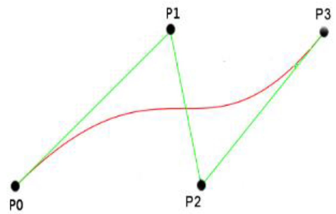
An n-degree Bezier curve is defined by (n + 1) control points. A three-degree Bezier curve will have four control points and a shape as shown in Figure 2, depending on the position of control points.
The shape functions of Bezier curves are Bernstein polynomials. The shape function is denoted by B i n , where
B i n = n i 1 t n i t i ,       i = 0 , 1 , 2 , 3 ;  
and n i = n ! i ! n i ! is the binomial coefficient.
For a Bezier curve having n = 3:
B 0 3 = 1 t 3 ;     B 1 3 = 3 t 1 t 2 ;       B 2 3 = 3 t 2 1 t ;         B 2 3 = t 3
The Bezier curve associated with the given control points can be expressed as:
P t = i = 0 n P i B i n t
As such, a Bezier parameterization of an airfoil has control points that are only indirectly determined by the underlying aerodynamics.

1.3. Bezier-Parsec Parameterization

This method combines Bezier and PARSEC parameterization techniques, drawing on the advantages of both approaches. The Bezier–PARSEC parameterization uses PARSEC variables as parameters, which are used to define four separate Bezier curves. These four curves represent the leading and trailing edge of the camber line and thickness distribution. The Bezier–PARSEC parameterization uses second-order continuity to join the leading and trailing edges. Bezier–PARSEC parameterization is denoted by BP ijkl, where i and j represent the order of the leading and trailing edge of the thickness curve, and k and l represent the order of the leading and trailing edges of the camber curve. Bezier–PARSEC parameterization increases the robustness and convergence speed for aerodynamic optimization using genetic algorithms.

1.4. BP 3333 Parameterization

All four curves of the Bezier–PARSEC Parameterization, i.e., leading and trailing edges of the thickness curve and leading and trailing edges of the camber curve, are defined by polynomials of the third order. Parametrically a third-degree Bezier curve is given by:
x u = x 0 1 u 3 + 3 x 1 u 1 u 2 + 3 x 2 u 2 1 u + x 3 u 3 y u = y 0 1 u 3 + 3 y 1 u 1 u 2 + 3 y 2 u 2 1 u + y 3 u 3
where u varies from 0 to 1. The BP 3333 parameterization depends on the 12 aerodynamic parameters shown in Figure 3. There are no free Bezier points in BP 3333.
The control points are given by:
Leading edge thickness curve
x 0 = 0 ;             x 1 = 0 ;                                                                 x 2 = r t ;                 x 3 = x t ; y 0 = 0 ;           y 1 = 3 k t x t r t 2 / 2 + y t ;         y 2 = y t ;               y 3 = y t ;
Trailing edge thickness curve
x 0 = x t ;     x 1 = 2 x t r t ;   x 2 = 1 + d z t e 3 k t x t r t 2 / 2 + y t c o t β t e ;   x 3 = 1   ; y 0 = y t ;           y 1 = y t ;             y 2 = 3 k t x t r t / 2 + y t ;                                                                                         y 3 = d z t e ;
Leading edge cambers curve
                                        x 0 = 0 ;             x 1 = r c c o t γ l e ;                 x 2 = x c 2 r c y c / 3 k c ;                 x 3 = x c ; y 0 = 0 ;               y 1 = r c ;             y 2 = y c ;                                                                               y 3 = y c ;
Trailing edge camber curve
x 0 = x c ;             x 1 = x c + 2 r c y c / 3 k c ;         x 2 = 1 + Z t e r c c o t α l e ;       x 3 = 1 ; y 0 = y c ;               y 1 = y c ;                                                                             y 2 = r c ;                                                                         y 3 = Z t e ;
These two techniques combine the advantages of both methods. The BP 3333 technique rapidly converges due to the smaller number of parameters involved. However, BP 3333 does not control the trailing edge in detail due to a smaller number of parameters. The BP 3434 technique (here not reported) overcomes the drawback of BP 3333, but convergence speed reduces due to a more significant number of variables. High-speed digital computers can compensate for the slow convergence rate of BP 3434. Hence, BP 3434 can be effectively applied for the optimization of an airfoil.
In this work, a novel approach is presented for the airfoil parametrization. The approach takes into account the currently available methodologies but, at the same time, gets closer to real design applications and aircraft geometrical/functional configuration, relying upon a mathematical model that:
  • easily allows airfoil shape morphing for leading edge/trailing edge rotation (global morphing) and skin deformation (local morphing).
  • easily enables the identification of functional areas and their contribution evaluation to the forces involved in the physical phenomena under analysis.
  • easily allows the application of geometric constraints.
  • involves a limited/reduced number of parameters for airfoil representation.
  • is eligible/suitable for developing aerodynamic, structural, or FSI optimization design processes on existing wing aircraft airfoils to evaluate the opportunity for morphing technology implementation [4].
In the proposed methodology, the airfoil mathematical representation is not based on a classical airfoil identification that includes the superposition of camber and thickness distributions and does not focus on the classical engineering parameters as in the PARSEC airfoil parameterization method. The 2D airfoil is partitioned in three sections [5]: central box, leading and trailing edge. Each of these three main sections is mathematically represented by two opposed, hand-side, uniform, non-rational B-spline curve segments describing the upper and lower segments’ perimeter. The curves continuity between two connected segments, belonging to two different sections, is ensured up to the 2nd derivatives. The originality of the approach used for the parameters setting consists in ensuring both the desired curve continuity and sufficient model freedom and flexibility with a limited number of variables, thanks to the introduction of tangent and curvature vectors scale factor parameters allowing for:
  • variables separation during the geometric fitting process.
  • smooth modification of the geometry of curved segments’ edges.
Relying upon variable separation, the geometric fitting procedure can be carried out innovatively considering two nested optimization processes, the first based on a genetic algorithm and the second based on numerical gradient evaluation of the objective function.
The airfoil representation method has been verified against different profiles, comparing the points and aerodynamic properties of the input profile and its model-based generated airfoil. A comparison between the geometrical approximation performance of the proposed method and the existing ones has been performed considering the parameterizations results reported in [2]. Each segment’s contribution to the aerodynamic force has been evaluated. This contribution has been decomposed in the direction of the asymptotic velocity and of its normal, to determine the lift and drag components for both unmorphed and morphed shapes. Finally, an example of global and local morphing CFD optimization process results has been provided to show possible applications of the airfoil mathematical model.

2. Descriptions of the Methodology

The procedure defining the 2D airfoils mathematical model with a reduced number of parameters is summarized in the flowchart described in Figure 4.
Each flowchart step will be described in detail in the subsections of this paragraph. The first step considers the input of a 2D airfoil whose geometric perimeter is represented by Cartesian coordinate pairs, detailed in Section 2.1. The second step deals with the partition of the input airfoil into sections and again the partition of each section into segments, upper and lower ones, presented in Section 2.2. In the third step, described in Section 2.3, each single airfoil segment is mathematically represented by B-spline curves. The considered curve parameters are the control points (CPs), whose number can be reduced with the introduction of scale factor parameters (SFs). The fourth step considers how the geometric boundary conditions have been applied at the extremity of each segment, in Section 2. The fifth step describes the procedure to evaluate each segment parameter, valid for the entire airfoil model representation, in Section 2.5.
The airfoil mathematical model and the aerodynamic analysis have been developed considering the MATLAB R2022a update 3 [6], the open-source Xfoil 6.99 software [7], and the Octave Nurbs package software [8]:
  • MATLAB is the main software for implementing optimization algorithms and for calling the CFD Xfoil 6.99 code inside the optimization loops.
  • Xfoil 6.99 is the aerodynamics solver for evaluating the 2D airfoil aerodynamic properties.
The hardware used for all the performed simulations is an AMD 3.80 GHz and 16 GB RAM.

2.1. Input 2D Airfoil

The input airfoil is given by points in the 2D Cartesian coordinate system P(xi, yi), i = 1, …, n, representing the airfoil perimeter. The P(xi, yi) coordinates are provided counterclockwise, starting from the trailing edge and following the airfoil’s upper side, then coming back to the trailing edge following the airfoil’s lower side. The input airfoil points can be taken from different sources:
  • from the University of Illinois at Urbana-Champaign Dept. of Aerospace Engineering website, in particular from the UIUC Airfoil Data Site website section [9,10];
  • from the book “Theory of wing sections” [11];
  • from the library of the Xfoil 6.99 software geometric tool [12].
Three airfoils have been chosen for verifying the mathematical model capability to represent different airfoil geometries, starting from a symmetric one: NACA 0012, NACA 23012, and NREL’s S809. In addition, three airfoil geometries have been reduced with the proposed method to perform a comparison with existing methods: RAE2822, NACA 0406, NACA 0160.

2.2. Airfoil Partitioning

The airplane wing usually is characterized by three functional areas: the central box (CB), which can be considered fixed without any morphing ability due to structural constraints; the forward, leading edge (LE), and backward extremity, trailing edge (TE), areas with geometric modification capabilities. It has been therefore decided to partition the airfoil into three sections with the opportunity for the user to define the partition intervals so that the morphing portion can increase or decrease due to design choices. In the following, the LE, CB and TE have been defined by the chord percent partition points at [0.0 0.3 0.7 1.0], but the user could modify these values if necessary:
  • LE section starting from the airfoil point P(x, y) of minimum x coordinate up to the 30% of the airfoil chord: 0 ≤ x/c ≤ 0.3.
  • CB section starting from 30% up to 70% of the airfoil chord: 0.3 ≤ x/c ≤ 0.70.
  • TE section starting from 70% up to 100% of the airfoil chord: 0.70 ≤ x/c ≤ 1.
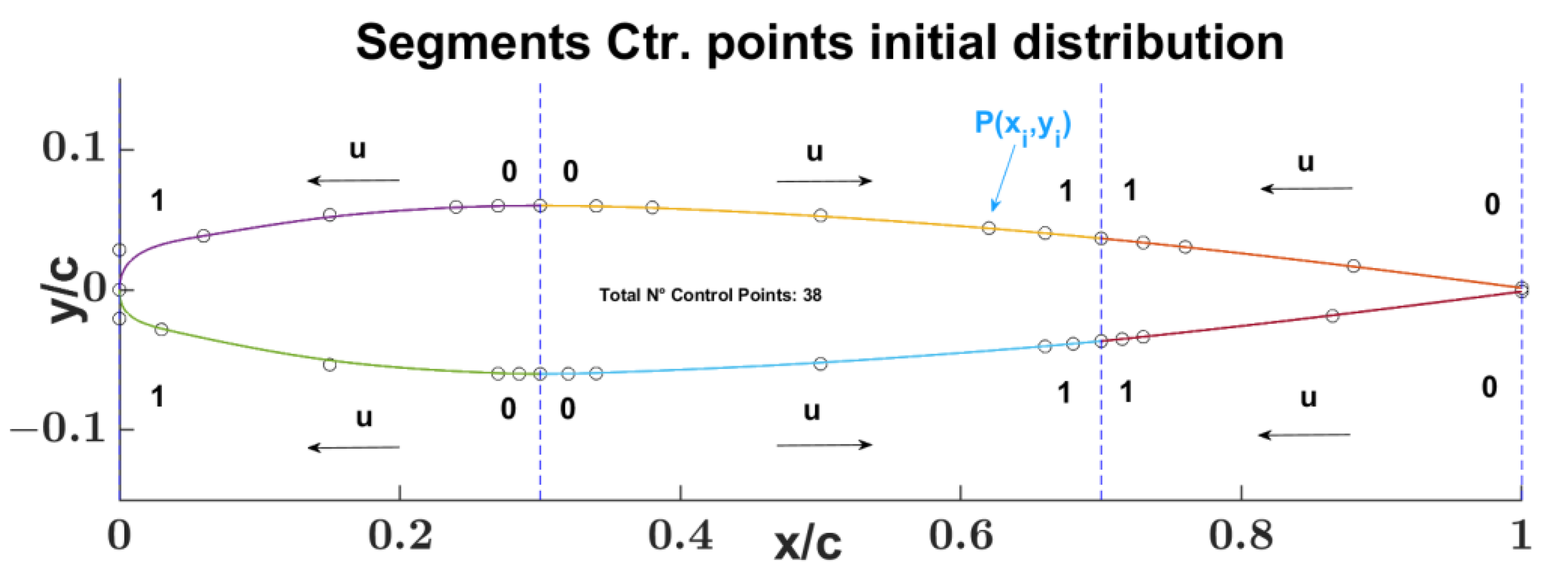
During the partition phase, if partition points are not already present among the input airfoil data, they are included, and the closest points, within a Euclidean distance tolerance of ±1 × 10⁻³, are removed. Each zone is characterized by two curve segments: the upper and the lower, for a total of six curve segments. The partition points identify the curve segments’ extremities. The consecutive segments are connected at their extremity points, here referred to as joints, shown in Figure 5.
The output of the airfoil partitioning phase consists of the partition of the input airfoil Cartesian coordinates into 6 segments, each with two joints, belonging to 3 different sections. Table 1 describes the geometric segment topology of the partitioned airfoil.

2.3. Mathematical Airfoil Segments Representation

For this work, a parametric representation [13] of the curve segments was selected, and, without loss of generality, the u parameter domain can be considered normalized to [0 1]:
C(u) = (x(u), y(u))             0 ≤ u ≤ 1
with C(u) indicating a uniform, non-rational B-spline (UNRBS) [13].

2.3.1. UNRBS

The general definition of UNRBS curves is:
C u = i = 0 n N i , p u P i         1   u 0
U = u 0 , , u m = 0 , , 0 p + 1 , u p + 1 , , u m p 1 , 1 , , 1 p + 1 where   m = n + p + 1
where: Pi are the n control points (forming a control polygon); {Ni, p(u) } are the pth-degree (order p + 1) B-spline basis functions in general defined on the non-periodic and nonuniform knot vector U whose parameter values u (u0 < u1 < …ui < 1) are called breakpoints. The segments, denoted by Ci(u), 1 ≤ i ≤ m, are constructed so that they join with some level of continuity not necessarily the same at every breakpoint.
The ith B-spline basis function of p-degree (order p + 1), denoted by Ni, p(u), is defined as
N i , 0 = 1   i f   u i u u i + 1 0   otherwise
N i , p = u u i u i + p u i N i , p 1 u + u i + p + 1 u u i + p + 1 u i + 1 N i + 1 , p 1 u
The UNRBS is a non-rational pth-degree B-spline curve characterized by U knot vector break points’ uniform distribution, as shown in Figure 6.
The considered UNRBS is the cubic one, p = 3, and its mathematical representation is defined by:
C u = i = 0 n N i , p u P i           1   u 0
U = u 0 , , u m = 0 , 0 , 0 , 0 3 + 1 , u 4 , , u m 4 , 1 , 1 , 1 , 1 3 + 1 where   m = n + 4
N i , 0 = 1   if   u i u u i + 1 0   otherwise  
N i , 1 = u u i u i + 1 u i N i , 0 u + u i + 2 u u i + 2 u i + 1 N i + 1 , 0 u
N i , 2 = u u i u i + 2 u i N i , 1 u + u i + 3 u u i + 3 u i + 1 N i + 1 , 1 u
where
u k u k 1 = Δ u   =   cos t               k = 4 m 3
Δ u   = 1 / m 1
The uniform knot vector breakpoints distribution and the alternate segment parametric curve orientation (see Section 2.3.3) provide a sort of “symmetry” to the airfoil mathematical model representation. This mathematical configuration provides a more regular curve behavior at the neighbor segments’ point of connection, reducing the possible collapsing and x-coordinate inversion of the control points during the geometry morphing.

2.3.2. Curve Derivatives in Parametric and Cartesian Formulation & SF Parameter

The 1st curve derivative in parametric (tangent vector) and Cartesian formulation can be written as follows [14]:
C u = C x u   ,   C y u   = x u ,   y u = dx du , dy du ;
  y x = dy dx = dy du du dx =   y u   x u = C y u C x u
Multiplying the C’(u) vector by a scale factor parameter (SF), the value of the 1st derivative does not change:
SF   C u = SF   C x u   ,   C y u   = SF   x u ,   y u = SF dx du , dy du ;
y x = SF   C y u SF   C x u = y x .  
The curve’s 2nd derivative in parametric (tangent vector) formulation can be written as:
C u = C x u   ,   C y u   = x u ,   y u = d 2 x du , d 2 y du ;
y x = d 2 y dx = d du dy du du dx du dx = d du C y u C x u 1 C x = dC y du 1 C x 2 + C y C x d du 1 C x
Then, considering y’(x) as function of C’(u):
y x = C y C x y C x 2 = C y C x C y / C x C x 2
Multiplying the curvature vector C″(u) by the scale factor parameter (SF) used for the tangent vector C′(u), but this time squared, the value of the 2nd derivative does not change:
SF 2   C u = SF 2 C x u   ,   C y u   = SF 2 x u ,   y u = SF 2 d 2 x du , d 2 y du ;
Considering the scaled tangent vector SF C′(u), it results:
y x = SF 2   C y SF 2 C x y SF   C x 2 = C y C x   C y / C x   C x 2 = y x

2.3.3. UNRBS Boundaries Control Points in Terms of C′ C″ and SF

The 1st and 2nd vector derivatives at the extremities curve segment (u = 0, u = 1) can be expressed in terms of the UNRBS parameters (control points Pi, breakpoints {ui}, p curve degree):
C 0 = p u p + 1 P 1 P 0 ;
C 1 = p 1 u m p 1 P n P n 1 ;
C 0 = p p 1 u p + 1 2 P 0 p p 1 u p + 1 1 u p + 2 1 u p + 1 P 1 + p p 1 u p + 1 u p + 2 P 2 ;
C 1 = p p 1 u m p 1 2 P n p p 1 u m p 1 1 u m p 2 1 u m p 1 P n 1 + p p 1 u m p 1 u m p 2 P n 2 ;
Given or assigned the:
  • extremities of the curve segment coordinates P0 = P(x0, y0) and Pn = P(xn,yn)
  • tangent vectors at the extremities of the curve segment C′(0) and C′(1)
  • curvature vectors at the extremities of the curve segment C″(0) and C″(1)
It is possible to evaluate the pair coordinates of the P1 = P(x1, y1) P2 = P(x2, y2) and Pn−1 = P(xn−1, yn−1)Pn−2 = P(xn−2, yn2) control points in terms of SF parameter:
P 1 = P 0 + u p + 1 p SF   C 0 ;
P n 1 = P n 1 u m p 1 p SF   C 1 ;
P 2 = p 1 u p + 1 P 0 p 1 1 u p + 2 1 u p + 1 P 1 + u p + 1 u p + 2 p p 1   SF   C 0 ;
P n 2 = p p 1 u m p 1 P n p 1 1 u m p 2 1 u m p 1 P n 1 + u m p 1 u m p 2 p p 1 SF   C 1 ;
Introducing the SF parameter, it is possible to modify the P1, Pn−1, and the P2 and Pn−2 control points’ position by varying the velocity and acceleration of the parametric curve segment at its extremities but keeping the same 1st and 2nd Cartesian derivatives values.

2.3.4. Segment Parameters

The airfoil, as seen in Section 2.2, is partitioned into three areas: LE, CB, and TE. Each area is delimited by two curve segments, the upper and lower, for a total of six segments. A single airfoil segment is mathematically represented by a uniform B-spline curve defined by the Control Points (CPs):
  • boundary control points (BCps).
  • interior control points (InCps).
The advantage of this approach is that free-form geometrical shapes can be represented with fewer design variables compared to the direct use of pairs coordinates.
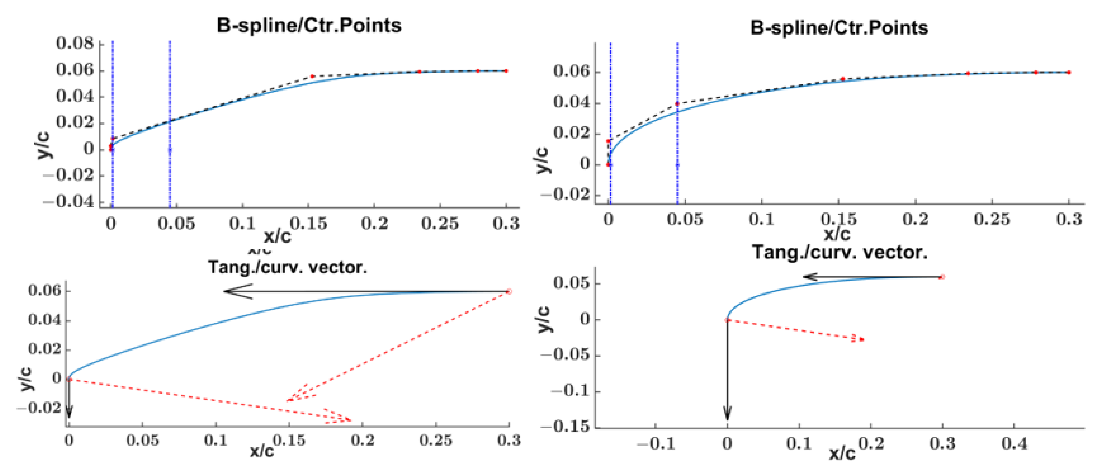
Each CP P(xi, yi) is characterized by two parameters, its Cartesian coordinates. Figure 7 shows an example of airfoil segment CPs distribution and the considered B-spline u parameter orientation. Figure 8 shows the tangent curvature vectors at the segment 5 extremity points.
The BCPs are useful to define the position of the segment extremities and the related tangent (C′) and curvature (C″) vectors. The number of BCPs can vary on each segment extremity from 1 up to 3 depending on the geometric condition to be imposed: 1 BCP for C0 continuity; 2 BCPs for C1 continuity; 3 BCPs for C2 continuity. The InCPs are all the CPs located between the two boundaries of CP groups. Table 2 and Table 3 summarize, in segment-wise order, the number of parameters for C0 and C2 segment boundary condition requirements related to the limit cases; this is done by specifying the:
  • boundary conditions assigned at the extremities of each segment: C0 up to C2 continuity.
  • required number of BCPs to satisfy the boundary conditions.
  • desired number of InCPs.
The positions of the extremity points of the segment curves were assigned during the partition phase, so the BCPs at the segment extremities do not have to be considered as variables. Table 2 shows that the required number of parameters for describing the partitioned airfoil geometry, ensuring the C0 continuity condition between the segments, is 52. In this case, the mathematical model is more flexible but unable to resolve the 1st and 2nd derivative discontinuities at the segment joints. From Table 3, it is possible to see that the number of parameters useful for describing the partitioned airfoil geometry, ensuring the C2 continuity condition between the segments, is 12. In this case, the mathematical model is less flexible.
By adjusting the parameters topology of each segment, it is possible to get a more or less complex mathematical model between the two limiting cases and represent a wide range of 2D airfoils for a design optimization process. The next subsection describes the parameters topology considered in this document.

2.3.5. Segments Reduced Parameters

A way to reduce the number of parameters of the mathematical model while simultaneously preserving its capacity to ensure the desired curve continuity and to describe a wide range of airfoil geometry families is to introduce the scale factor parameters (SFps).
The SFps are generally two for each segment, and one SFp for each extremity. By varying the SFps, it is possible to modify the position of the BCPs but, at the same time, to keep the same values for 1st and 2nd Cartesian derivatives of the segment curve, shown in Section 2.3.2 as Equations (25) and (30), and to satisfy the desired boundary conditions at the segments’ extremities. In the following Table 4, each segment’s parameters and boundary conditions are summarized for the reduced case.
The number of parameters has been reduced from 52 to 22, Table 4, no longer considering the BCPs parameters but considering the SFs parameters in their place. The upper and lower SFs boundary limits have been evaluated by imposing the max min x coordinate range for the segment BCPs. In the end, the airfoil is represented by 2 SFps for the segments from 2 to 5, 1 SFp for segments 1 and 6, and the desired number of InCPs (minimum 1) for each segment ((x, y) coordinates parameters).
Table 5 reports the established BCPs x coordinate extremities intervals in terms of the percentage of the segment length and the related SFs upper and lower bounds for the NACA 0012 airfoil.
Figure 9 shows an example of the results obtained for the left side SFps upper and lower bounds of NACA 0012 segment 3 (upper LE segment).
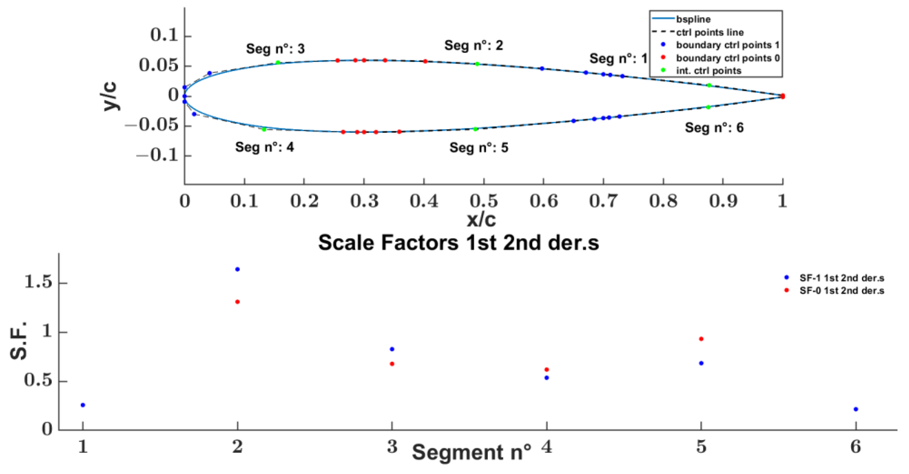
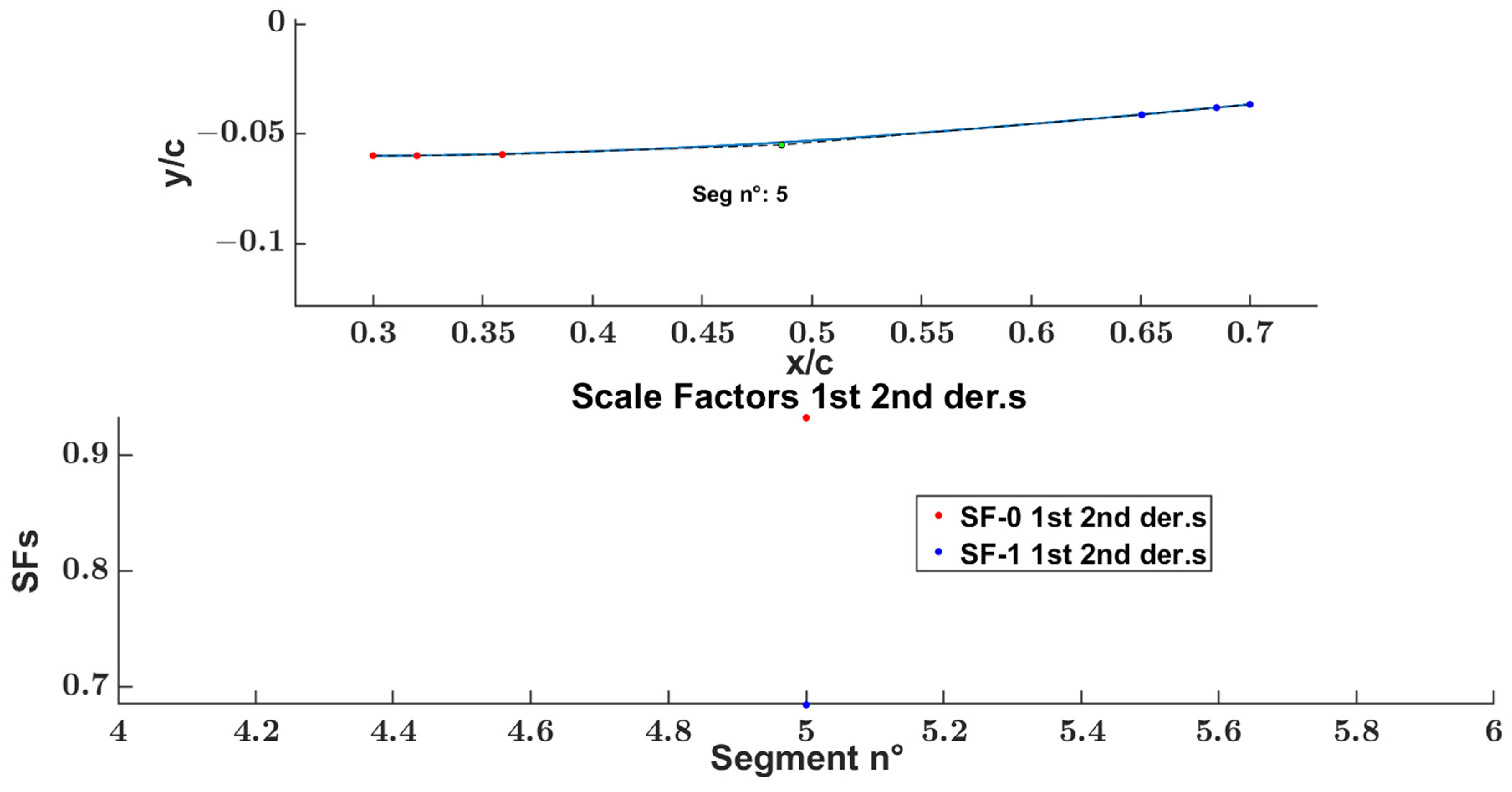
Figure 10 shows the NACA 0012 segments’ CPs distribution (BCPs and InCPs), and Table 6 the SFs values after an optimization cycle.

2.4. Segment Geometric Boundary Conditions

In Section 2.3.2, the 1st and 2nd Cartesian derivatives of the segment curve have been expressed as a function of the parametric C′ and C″ components; see Equations (23) and (28). To impose the desired continuity boundary condition at the segment extremities, it is necessary to evaluate the tangent C′ and curvature C″ vectors from the available data while taking into account the airfoil geometry partition topology, as shown in Table 1. To improve the segment curves’ smoothness at joint points, the C′ and C″ vectors at the extremities of the curve segments were evaluated by interpolating the input segment data through a B-spline interpolation routine and taking into account points from the neighbor segments.
A possible and currently implemented segment-wise strategy and priority sequence for the evaluation of the parameter and the geometric boundary conditions assignment is summarized in Table 7; even if the current choice of the parameter topology ensures the evaluation of the variables independently from the segment-wise priority and makes the same suitable for a parallel calculation.

2.5. Segment Fitting Procedure for Reduced Parameters

The fitting process aims to find the optimum parameter values for each UNRBS curve segment, minimizing the maximum Euclidean distances between the evaluated points and the related airfoil data points [15,16,17]. The reference data used to evaluate the parameters are the input airfoil points, segments-wise partitioned. The fitting process is composed of two phases:
  • 1st phase of pre-processing the airfoil data (Figure 11): this phase is characterized by three steps:
    • C′ and C″ vectors evaluation at each segment joint.
    • segments BCPs positioning in accordance with the C′ and C″ vectors.
    • SFps upper and lower bounds evaluation.
The C′ and C″ vectors can be evaluated by interpolating, through a B-spline interpolation routine, the input segment data airfoil points belonging to the neighbor segments, thus improving the smoothness of the curves at joints. Then, the BCPs 2D space positioning is evaluated according to Equations (35)–(38) of Section 2.3.3.
The segments SFps upper and lower bounds are evaluated considering the user-defined max/min x-coordinate range for the segment BCPs—see the example in Section 2.3.5—, as shown in Table 5. Algorithm 1 represents the pseudocode of the airfoil pre-processing phase.
Algorithm 1 [InitialAirfoil C′,C″,SF_lb, SF_ub]=Airfoil_preprocessing ( )
1Variable_Declaration ( )                            /* Airfoil global variable…definition*/
2File_Inizialization ( )                   /* fine name definition */
3Folder_Inizialization ( )               /* making working folders */
4Airfoil_Topology ( )                            /* x partitions, seg.s discretization
typology, fixed/free CPs,
x% seg. boundaries …definition */
5Airfoil_Load()                                    /* load target airfoil points, */
6Initial_Airfoil_PartitioningSeg( )         /* target airfoil partitioning */
7Create_Initial_B-pline_curves ( )         /* create segment b-spline curves */
8[C’,C″]=Segments_Joints_dC_ddC ( )    /*evaluating C’ & C″ vectors at
each joint from the target airfoil
points coordinates and apply
the same to the current airfoil
b-spline segments */
9[SF_lb,SF_ub]=Segment_bounds ( )     /* given the x% seg. boundaries the SFs upper and lowerboundaries are evaluated*/
10end Airfoil_preprocessing
  • 2nd phase segment reduced parameters evaluation (Figure 12): This step applies to all the segments whose C’ and C” extremity vectors are already known and assigned. The aim is to find the optimum segment UNRBS curve parameters that best fit the input segment airfoil points with the desired continuity boundary extremity conditions. Two nested optimization routines perform the parameter evaluations, an external and an internal one, considering the reduced segment parameters as variables, namely the SFs for the external routine, varying between the upper and lower bounds assessed in step 1, and the InCPs for the internal one. More specifically,
    • the external optimization cycle is based on a MATLAB genetic optimization function gamultiobj [18,19,20,21,22] dedicated to the two SFps only with two objective functions:
      obj1: sum((Euclidean distance between points).
      obj2: max(Euclidean distance between points).
      The two SFs parameters affect the position of the BCPs that define the lower and upper bounds of the interior CPs coordinates used for the inside optimization cycle.
    • the internal optimization cycle is based on MATLAB non-linear optimization fmincon [23,24,25,26,27] function involving the interior CPs parameters with:
      -objective function obj: minimizing the max (Euclidean distance between points);
      -upper and lower bounds: defined by the BCPs coordinates as a function of the SFps, output of the GA external cycle optimization.
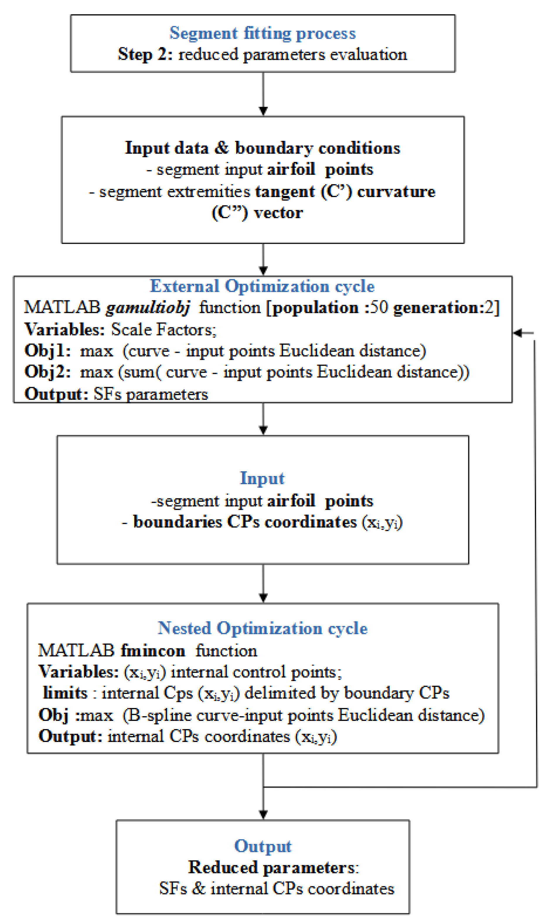
Figure 12. Segment fitting process, step2 flowchart.
Designs 07 00028 g012
Algorithms 2–4 are the segment fitting process step 2 pseudocodes and the setting of MATLAB external gamultiobj, nested fmincon algorithms.
Alghoritm 2 [InitialAirfoil]=Airfoil_Fitting_process (InitialAirfoil, C’,C″,SF_lb, SF_ub)
1For each curve segment
2[InitialAirfoil]=SegOptim_InCPs_SFs_nested_GA_Fmin(InitialAirfoil)
/* evaluation of segment SFps and InCPs
coordinates by:
                             - external gamultiobj
                             - nested fmincon
                              MATLAB algorithms */
3SaveAirfoil (InitialAirfoil);        /* save working InitialAirfoil variables*/
4Endfor
5end Airfoil_Fitting_process
Alghoritm 3 Matlab gamultiobj genetic algorithm settings
1[f1,f2]= fit_fcn (Airfoil current segment)   /*fitness function for evaluation
of two objective functions:
f1: max abs(Euclidean points distances);
f2: sum abs(Euclidean points distances);
fit_fnc calls the MATLAB fmincon
algorithm*/
/
2n_vars:= n_SFs                                    /* number of segment curve SFs */
3A = []; b = []; Aeq = [];beq = [];               /* linear constrains */
n_seg=current segment number             /* segment under fitting procedure*/
4lbGa= SF_lb (n_seg);                                 /*assign segment lower bound
ubGa= SF_ub(n_seg)                                 and upper bound*/
5[c,ceq]=nonlcon(Airfoil current segment)    /*check for avoiding b-spline
segment curve x coordinates
inversion*/
6 n_generationsGA=1; population_n=50;
opt = optimoptions(@gamultiobj,’PlotFcn’,’gaplotpareto’,
‘MaxGenerations’,n_generationsGA,
‘PopulationSize’,population_n,
‘PopulationType’,’doubleVector’
7[SFs_GA,fval_GA]=gamultiobj(fit_fcn,n_vars,A,b,Aeq,beq,lbGa,ubGa,nonlcon,opt)
8AirfoilPoints(InitialAirfoil);       /*update the segment curve geometry
properties and discretization*/
Alghoritm 4 MATLAB fmincon gradient based algorithm settings
1[BCPs0,InCPS0]=B-spline_SegmentCurve_updating(InitialAirfoil,
C′,C″,SF_GA)
2[y]=fit (InitialAirfoil)                    /* updating InCPsand B-spline cuve,
Evaluating objective function:
y=max(abs(Eucledian curve points
distance)) */
3IntCps0                                          /* initial internal control points*/
4A = []; b = []; Aeq = [];beq = [];
5 lb = flb(BCPs0); ub= flb(BCPs0)           /* InCPs upper and lower bounds
evaluated as function of the defined
boundary control points BCPs0 */
6[c,ceq]=nonlcon(Airfoil current segment)     /*check for avoiding b-spline
segment curve x coordinates
inversion*/
7opts = optimset(‘fmincon’, ‘TolFun ‘,1.e−12, FinDiffRelStep, 1.e−12);
8[InCP_fmin,fval_fmin]=fmincon(fit, InCP 0,A,b,Aeq,beq,lb,ub,[],opts);
9AirfoilPoints(InitialAirfoil);      /*update the segment curve geometry
properties and discretization*/
The reduced parameterization, as conceived, allows the parallelization of the single curve segment fitting process. Each segment fitting process is independent of the other ones. In the following subsection, an example of the results of the segment 5 (lower CB) fitting process of the NACA 0012 airfoil is reported.

Segments 5 (CB section) Fitting Process Results

Segment 5 belongs to the CB of the airfoil. The reduced SFps and InCPs can be evaluated by applying steps 1 and 2 of the segment fitting process:
  • The first step for evaluating the extremities boundary conditions, C’ C” vectors, and the SFps upper and lower bounds.
  • The second step for evaluating 4 reduced parameters: two (2) InCPs coordinates and two (2) SFps.
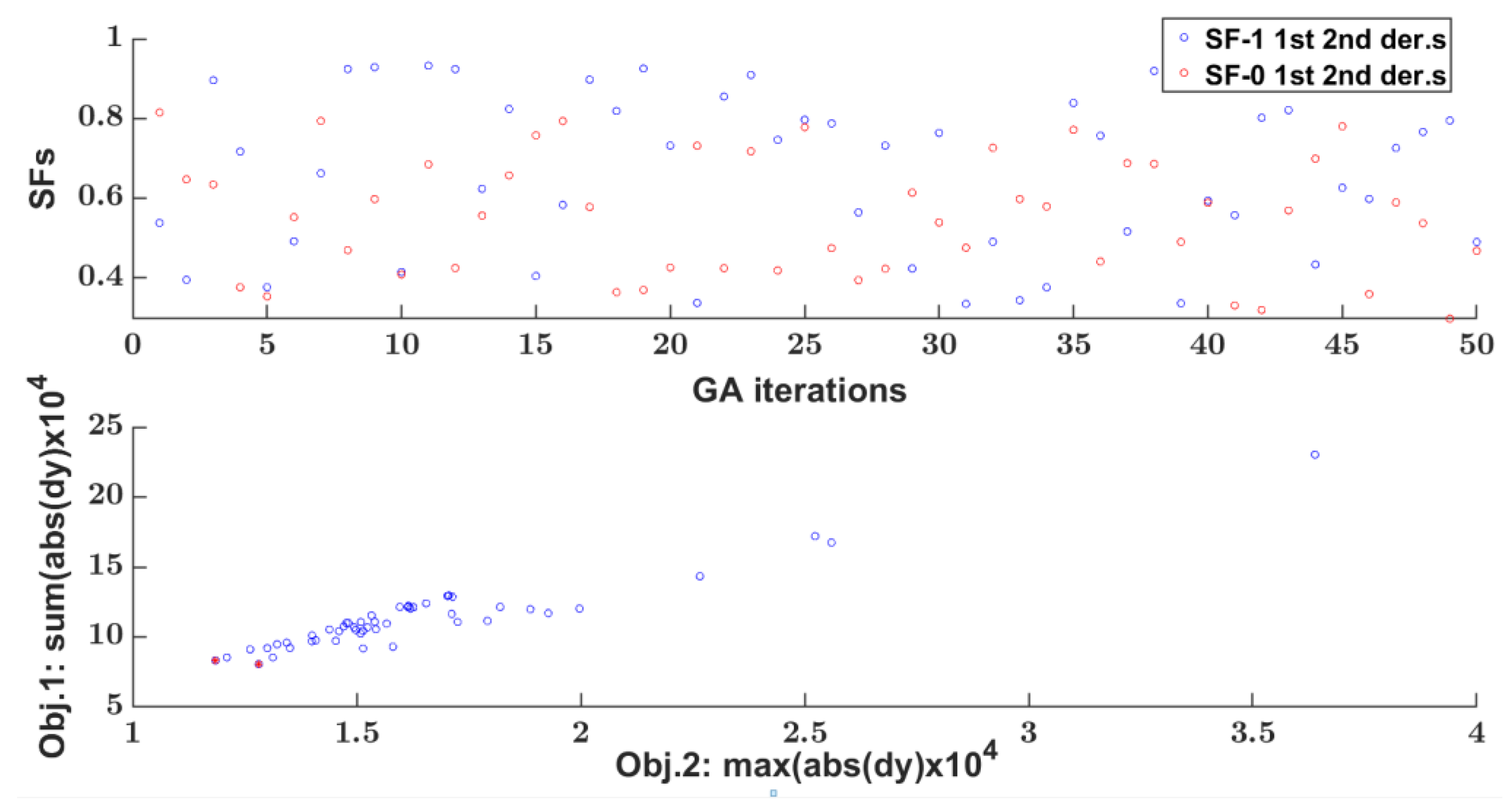
Figure 13 and Figure 14 show the NACA 0012 external genetic algorithm optimization iteration of the segment 5 step 2 for the SFps (1 generation with a population of 50) and the evaluated SFps optimum values.
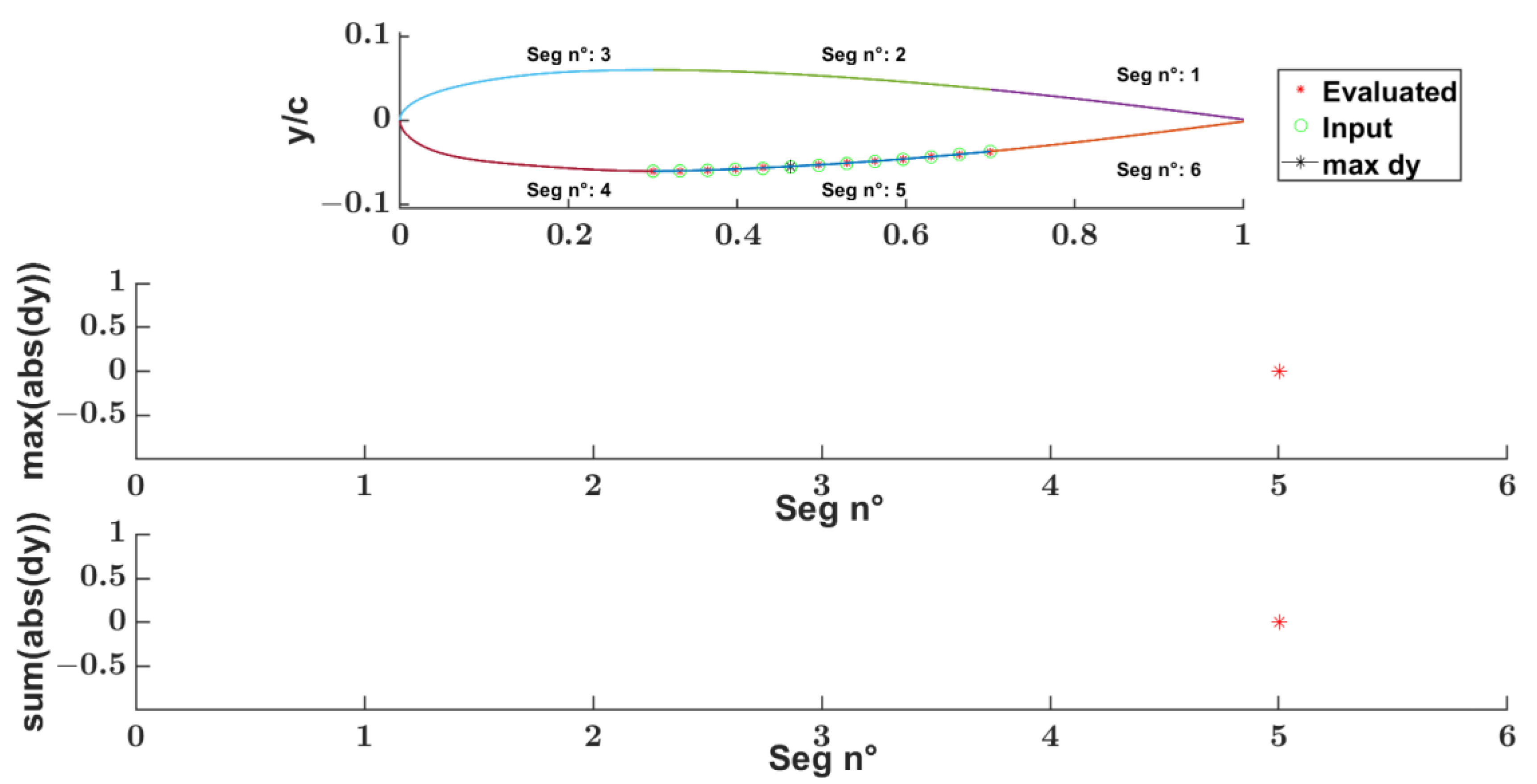
Figure 15 shows the NACA 0012 step 2 inside optimization algorithm iterations and optimum InCP parameters of segment 5, with the associated max geometrical error made on the same segment shown in Figure 16.

3. Results

The following Section 3.1, Section 3.2 and Section 3.3 shows a comparison between the geometric and aerodynamic properties of the input airfoil and the airfoil constructed by the mathematical model with reduced parameters: SFps and InCPs.
For each comparison, there are four typologies of figures:
  • geometrical input airfoil.
  • maximum Euclidean distance for each segment between the input airfoil and evaluated airfoil points.
  • the input airfoil aerodynamic properties compared with the evaluated airfoil properties considering two different discretizations: the input airfoil and an augmented one.
The analysis was performed on three airfoils to show the mathematical model’s capability to describe different 2D profile families. NACA 0012, NACA 23012, and NREL’s S809 airfoils were considered to validate the mathematical model with reduced parameters.
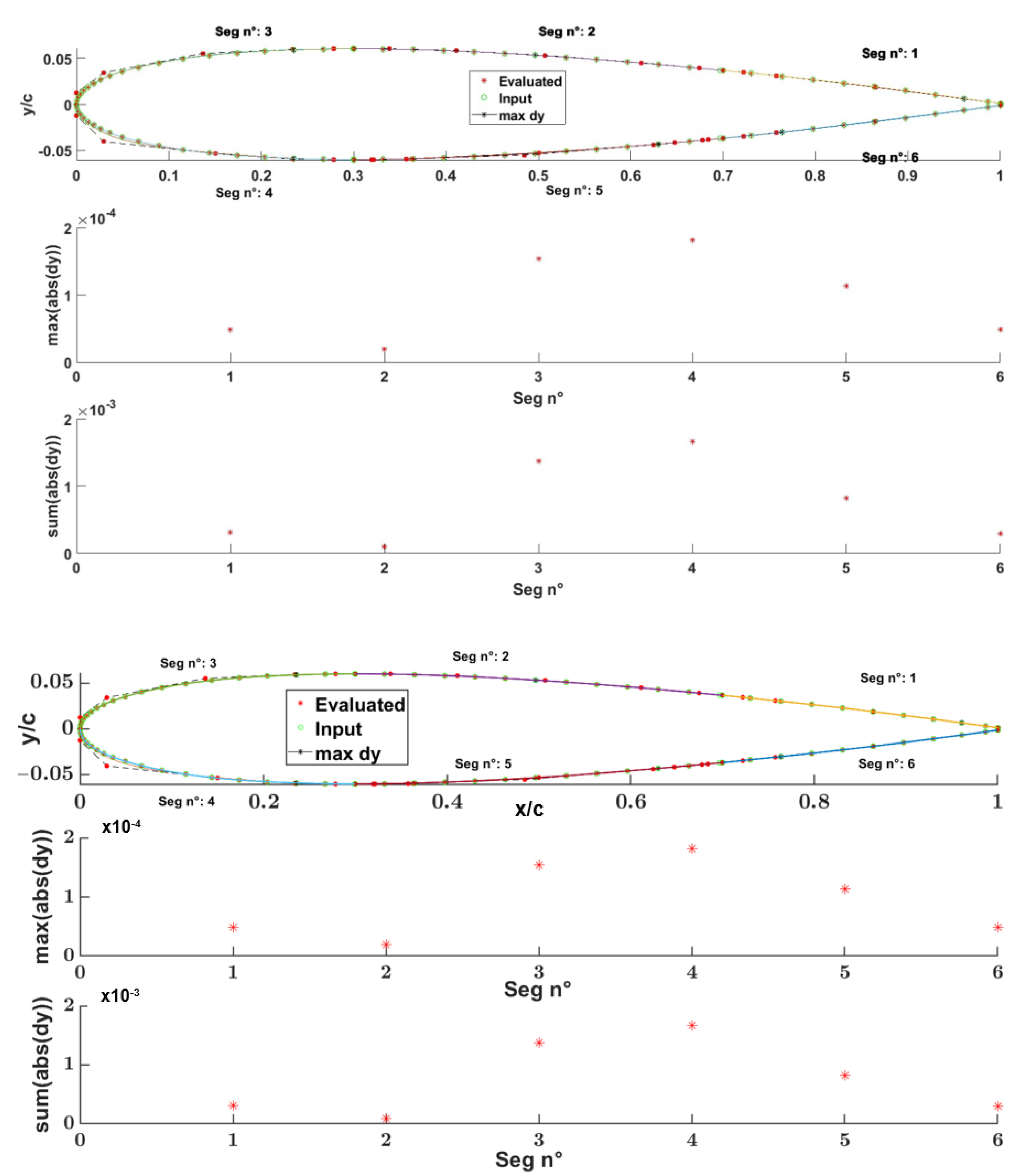
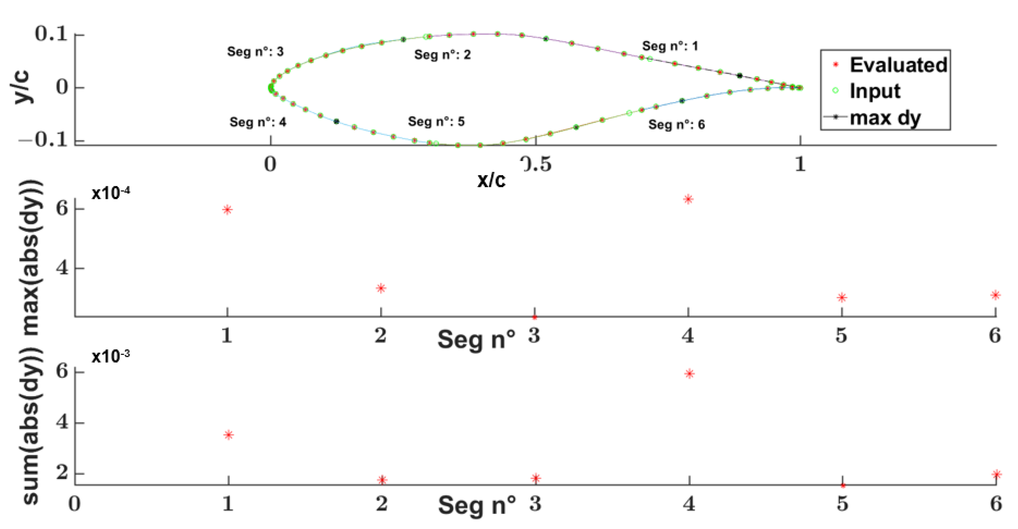
The geometrical maximum Euclidean distance observed in all the analyses was of the order O (10−4) and the aerodynamic properties of the evaluated airfoils with equal and increased discretization have all the same qualitative and quantitative behavior of the input airfoil aerodynamic properties. Table 8 reports the segment-wise and total timing required to evaluate the parameterized airfoil by a sequential calculation. Table 9 reports the segment-wise max Euclidean distance error and the sum of all absolute value Euclidian distance errors for each segment, where: max stay for maximum, abs absolute functions, and dy vertical abscissa difference.
The last Section 3.4 suggests a comparison between the results of target airfoils’ geometrical approximation performed by the methods described in [2], and the one herein proposed. The 2D profiles used for the comparison are the same as mentioned in the reference article [2]: RAE2822, NACA 0406, and NACA 0610.

3.1. NACA 0012

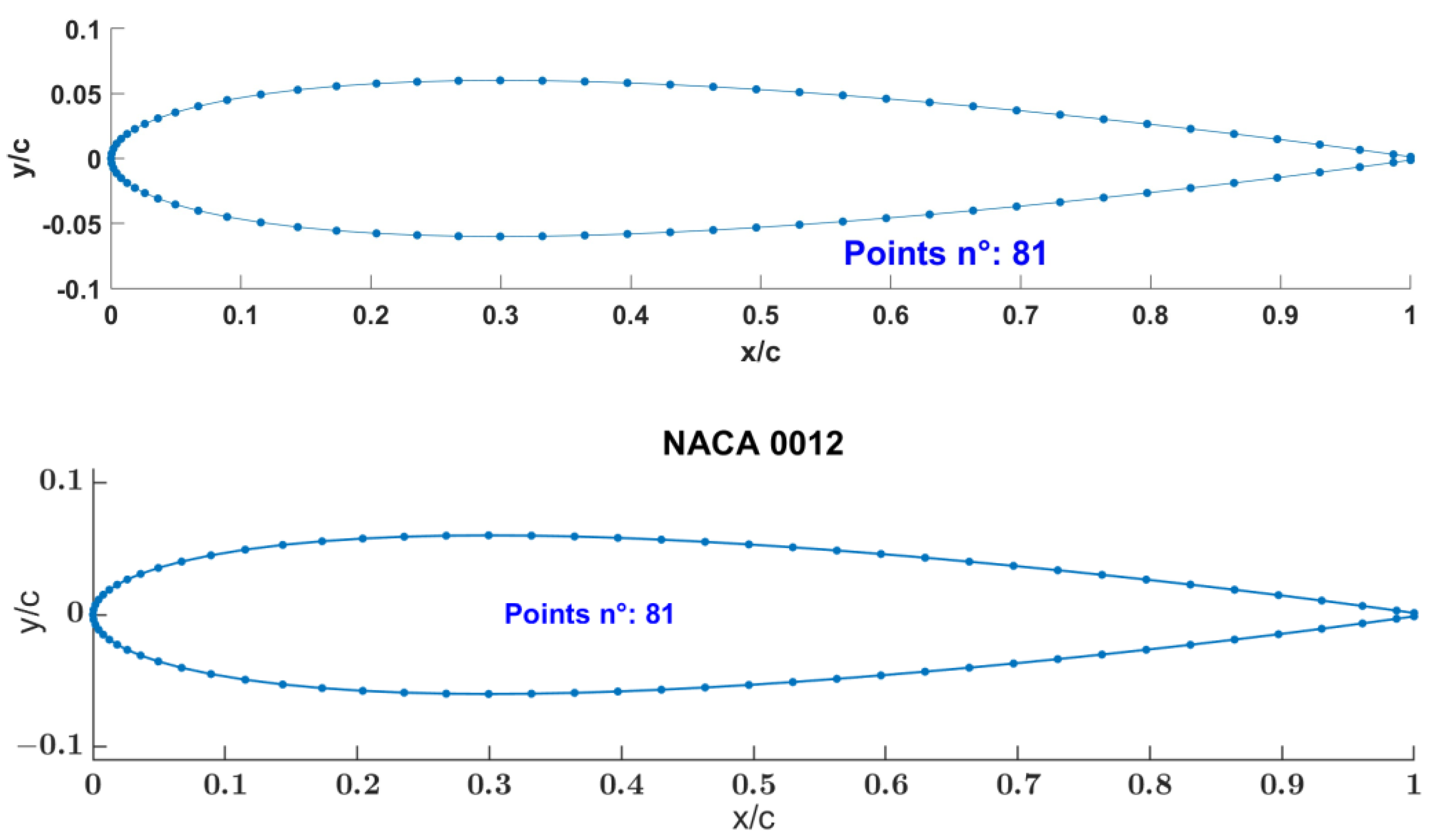
Figure 17 and Figure 18 show the target airfoil NACA 0012 and the segment-wise geometrical error (also reported in Table 9 column NACA 0012) between the input and parametrized profile.
Figure 19 shows the comparison of the aerodynamic curves c l α , c l c d   c m c l , E α = c l α / c d α between the target NACA 0012 and parametrized airfoil.

3.2. NACA 23012

Figure 20 and Figure 21 show the target airfoil NACA 23012 and the segment-wise geometrical error (also reported in Table 9 column NACA 23012) between the input and parametrized profile.
Figure 22 shows the comparison of the aerodynamic curves c l α , c l c d   c m c l , E α = c l α / c d α between the target NACA 23012 and parametrized airfoil.

3.3. NREL’s S809

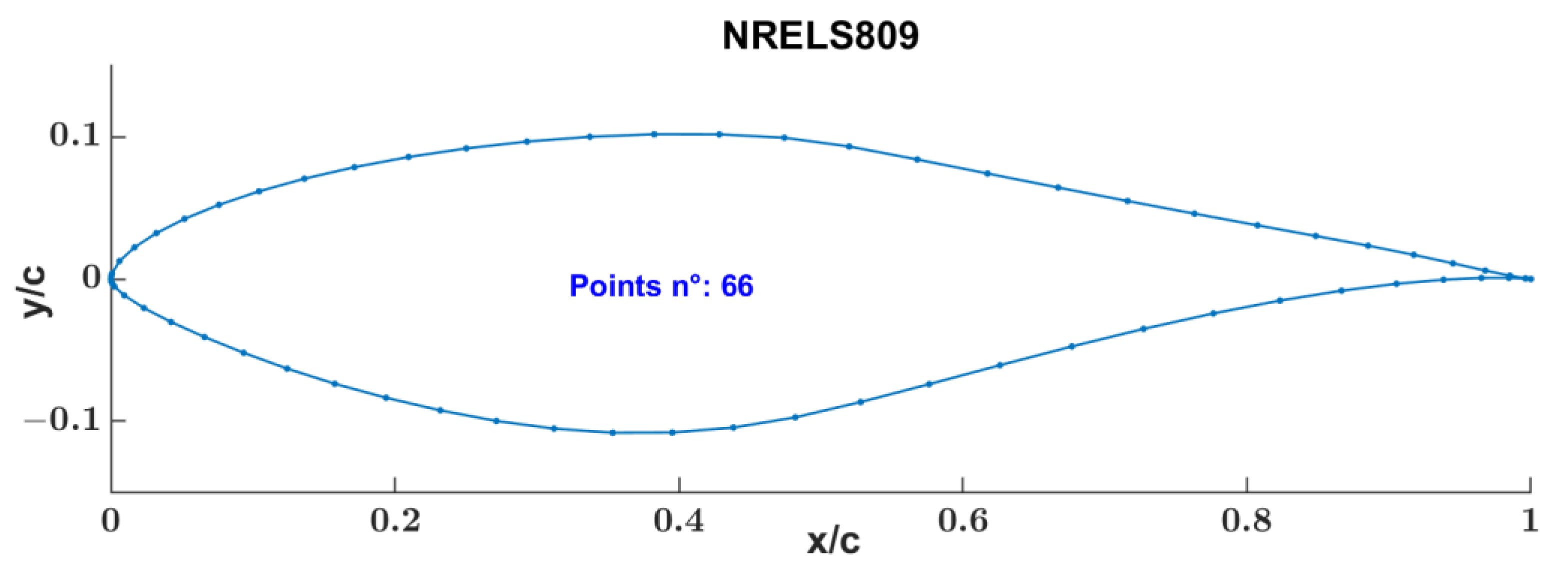
Figure 23 and Figure 24 show the target airfoil NLEL’s S809 and the segment-wise geometrical error (also reported in Table 9 column NLEL’s S809) between the input and parametrized profile.
Figure 25 shows the comparison of the aerodynamic curves c l α , c l c d   c m c l , E α = c l α / c d α between the target NREL’s 809 and parametrized airfoil.

3.4. Comparison between Existing Methods and the Proposed One

These airfoils RAE2822, NACA 0406, and NACA 0610 have been represented by the new mathematical model and both the fitting process segment-wise computation time and geometrical approximation have been evaluated, Table 10 and Table 11. Table 12 and Table 13 show that the proposed mathematical model performs better than the:
  • B-spline interpolation method for the considered number of parameters.
  • Numerical basis functions and B-spline interpolation methods for the geometrical approximation, which is more accurate by a magnitude.

4. Discussion

The B-spline curve segments are the basic geometric element in the airfoil representation and, at the same time, they describe the fundamental airfoil functional areas: LE upper and lower side, segments 3 and 4; CB upper and lower side, segment 2 and 5; TE upper and lower side, segment 1 and 6. In an optimization design process, it is possible to modify the shape of a single segment curve and/or more than one shape segment curve at a time, in order to modify the desired functional areas (LE, CB, TE), appropriately. As a consequence, in a design optimization process, it is useful to know the segment-wise aerodynamic force contribution at every iteration. The followings figures and tables show examples of:
  • two examples of segment-wise evaluation of pressure and skin friction forces and their contribution to the airfoil lift and drag.
  • global morphing CFD optimization” and the next “local morphing CFD optimization” for exploring a further improvement of the aerodynamic properties.
The NACA 23012, generated by the mathematical model defined in this paper, was considered for both the segment-wise aerodynamics properties evaluation and for an example of an aerodynamics design optimization process.

4.1. NACA 23012 Segments Wise Aerodynamics Properties Evaluation

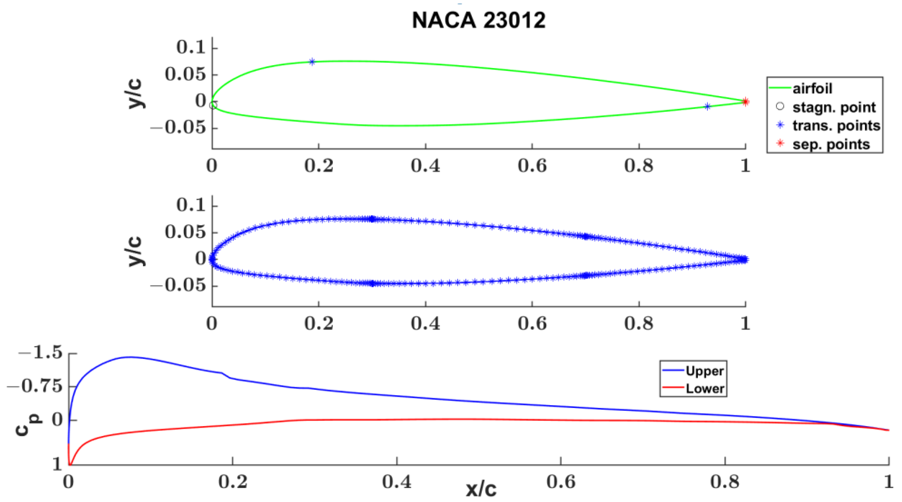
Figure 26 shows the NACA 23012 airfoil with the stagnation, transition, and separation points, its Chebyshev segment discretization and pressure coefficient distribution at Re 3.5 × 10⁶, α = 4 ° .
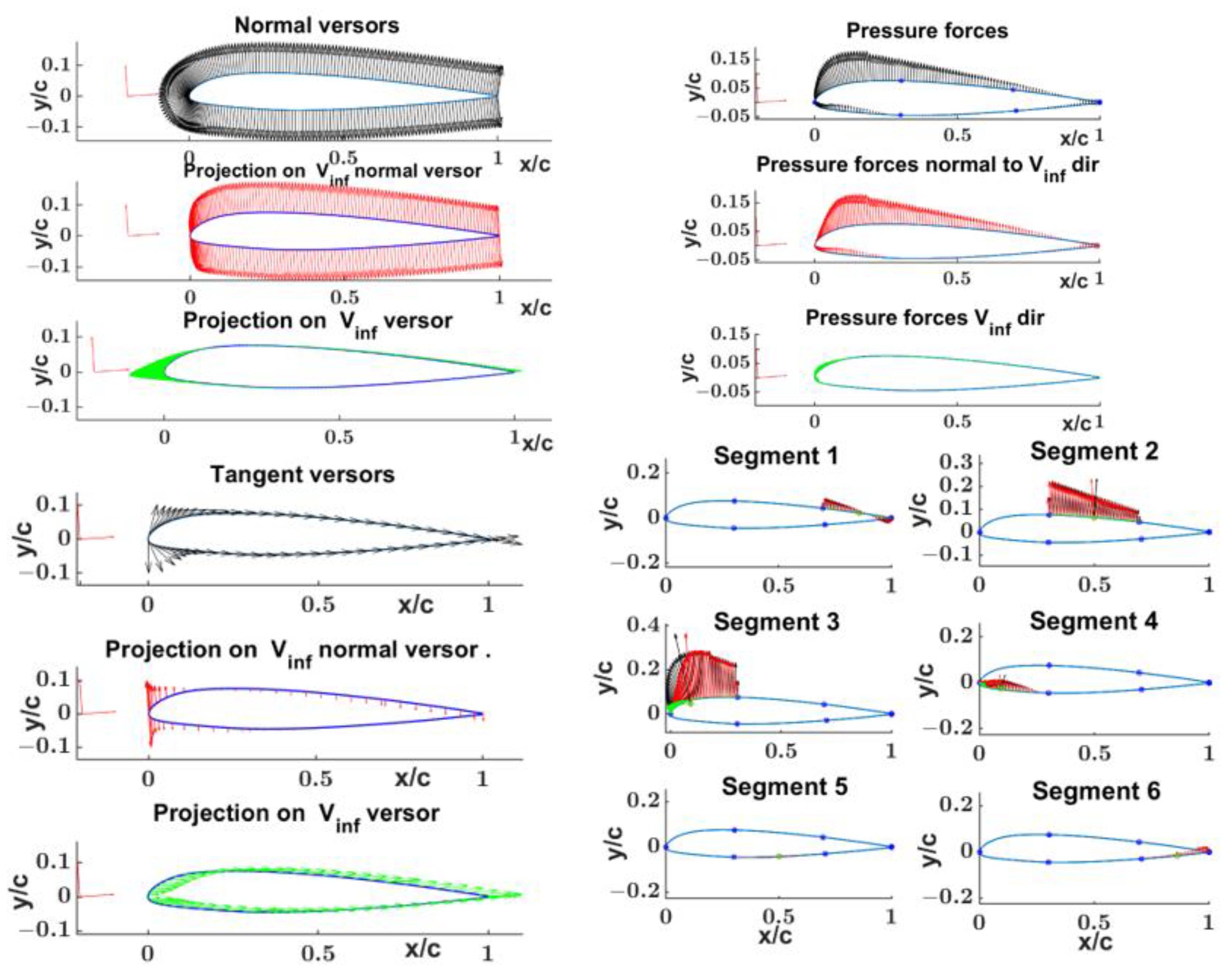
Figure 27 represents the normal and tangent vectors to the airfoil and their decomposition in the Vinf direction, and the one normal to it; the pressure forces, their segment-wise distribution, and decomposition along the Vinf direction, and the normal to it. The normal and tangent vectors and the curvilinear abscissa were used for the calculation of the pressure forces.
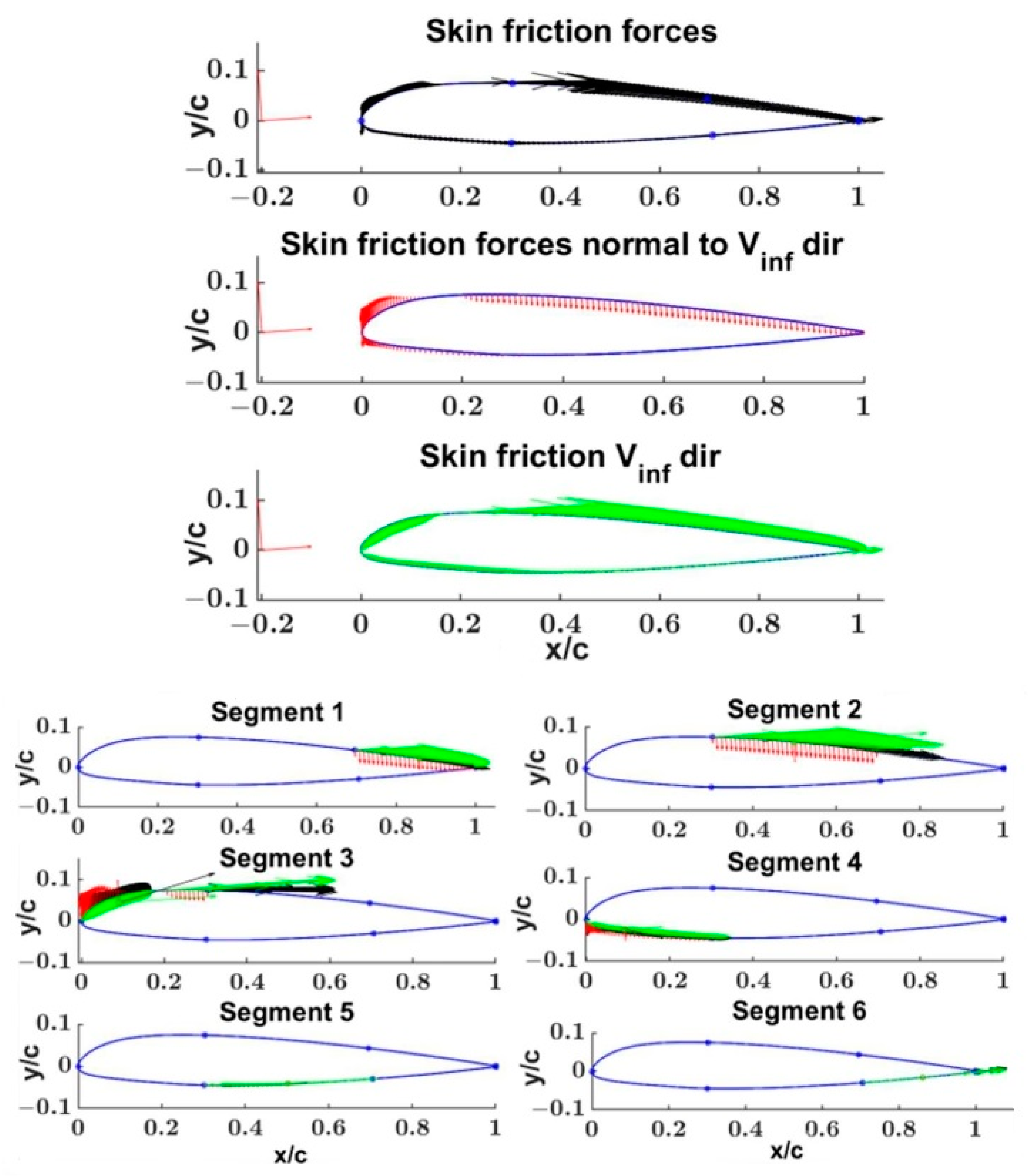
Figure 28 shows the airfoil friction forces, their segment-wise distribution, and their projection along the Vinf direction, and the normal to it.
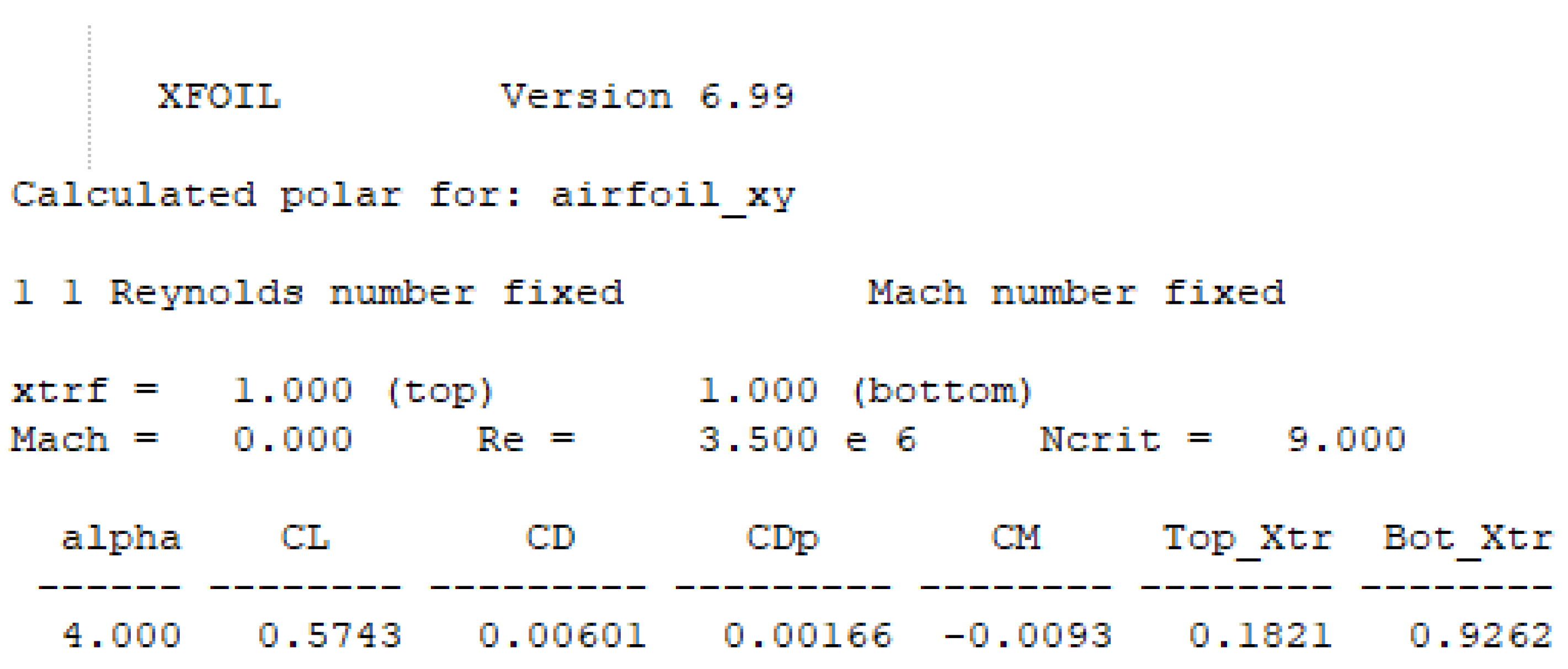
Quantitative Xfoil polar results are reported in Figure 29. Table 14 contains the segments lift (cli) and friction (cfi) coefficients. In particular, the last one is split into the components, computed along the Vinf direction and its normal. Note that the shape drag (cdp) is deduced from the difference between cd and cdf (cdp = cd − cdf) instead of being calculated via surface pressure integration due to the presence of numerical noise.

4.2. Morphed NACA 23012 Segment-Wise Aerodynamic Properties Evaluation

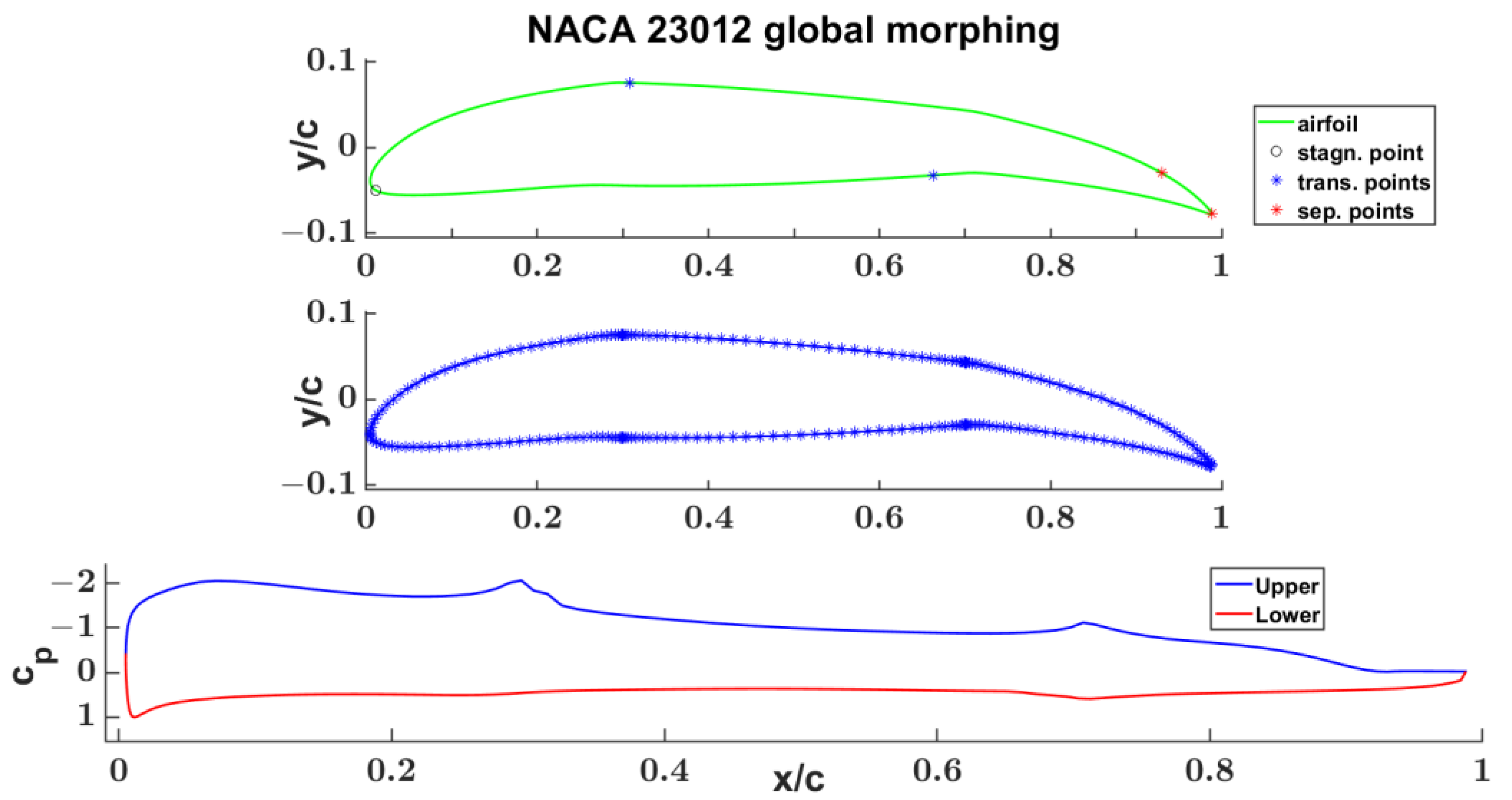
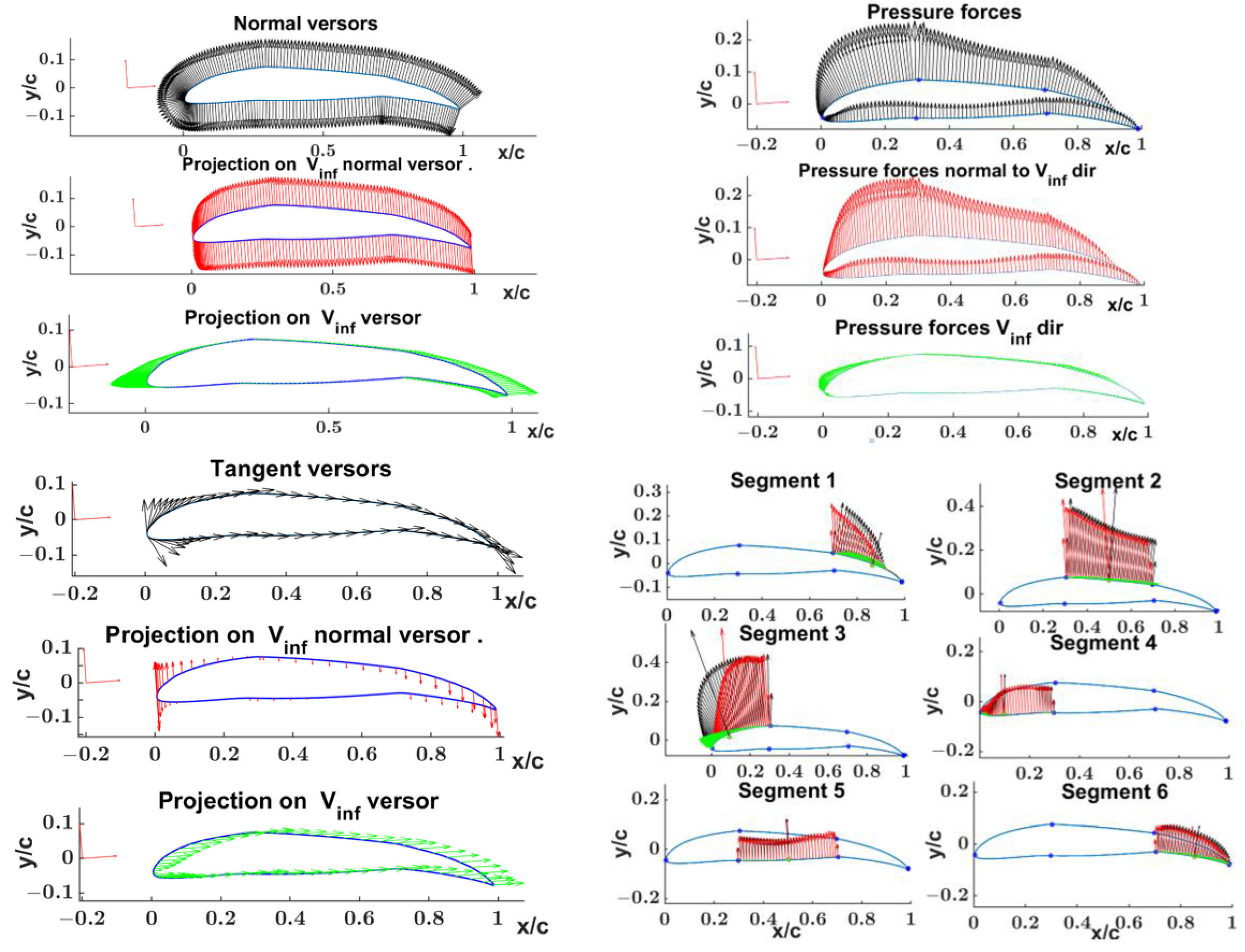
Figure 30 shows the NACA 23012 global morphed geometry, obtained by the LE and TE rotation around the 0.3 and 0.7 section middle points with the stagnation, transition, and separation points, its Chebyshev segments discretization, and its pressure coefficient distribution always for Re 3.5 × 10⁶, α = 4 °
In Figure 31, the normal and tangent vectors to the airfoil and their components along the Vinf direction and its normal; the pressure forces, their segment-wise distribution, and decomposition along the Vinf direction, and the normal to it are represented. The normal and tangent vectors and the curvilinear abscissa were used for the calculation of the pressure forces.
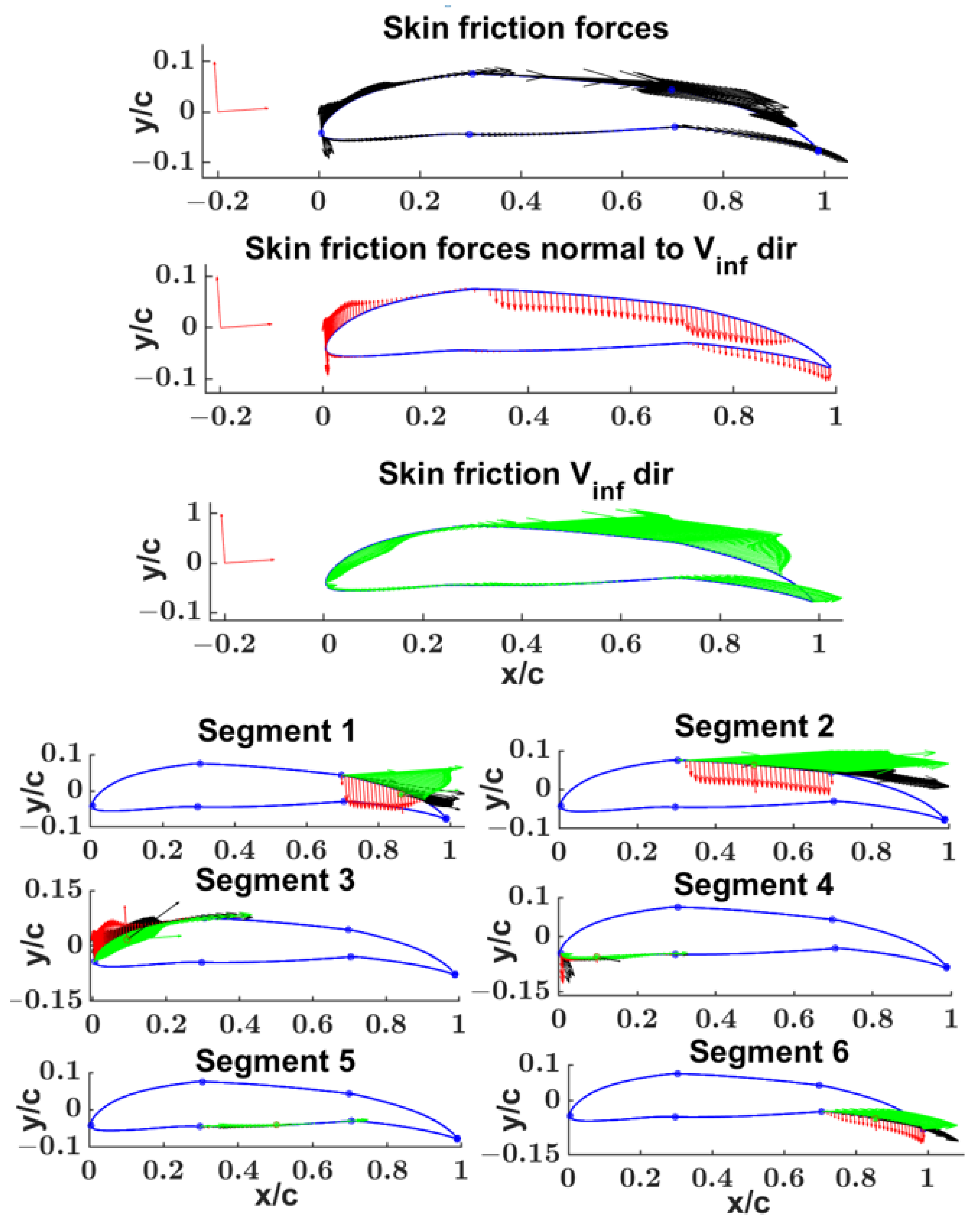
Figure 32 shows the segment distribution of the friction forces, their resultants, and their decomposition along the Vinf direction and its normal. forces.
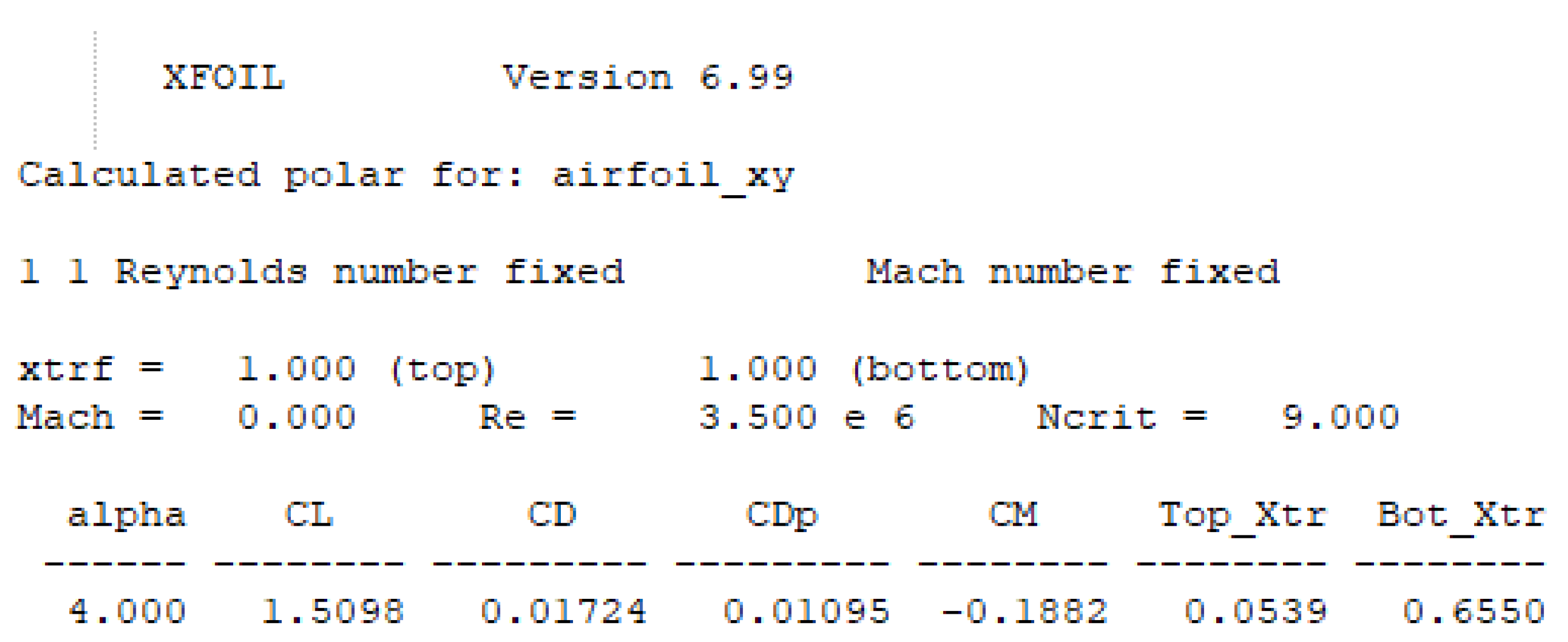
Quantitative Xfoil aerodynamic results are reported in Figure 33. Table 15 contains the lift (cl) and friction (cf) coefficients, computed at each segment. In particular, the last one is split into the contributions computed along the Vinf direction and its normal. Note that, as before, the shape drag (cdp) is deduced from the difference of cd and cdf (cdp = cd·− cdf), instead of being calculated via surface pressure integration due to the presence of numerical noise.

4.3. NACA 0012 CFD “Global & Local” Morphing CFD Design Optimization

The airfoil mathematical model allows easy global and local section/segment morphing and is suitable for use in a design optimization process.
Global section morphing is intended as section rotation, obtained by acting on segments 1, 6, and their BCPs and InCPs parameters for TE rotation; segments 3, 4, and their BCPs and InCPs parameters.
Local section morphing is intended as segment skin deformation obtained by acting on SFps and InCPs parameters with a “limited variation” defined by the user.
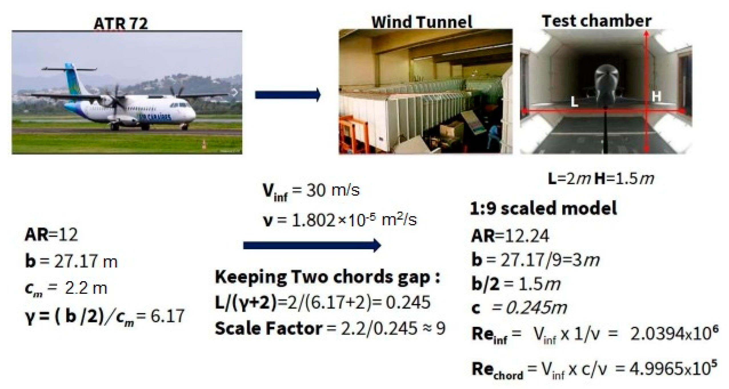
We could consider an example of design optimization of a scaled NACA 23012 which can be considered a root section of a rectangular wing useful for a wind tunnel test. The airfoil was scaled by a scale factor of 9 taking into account the aircraft typology and test chamber dimension. See Figure 34 for a detailed consideration of scale factor evaluation.
Following the procedure described in Section 2.5, the parameterized airfoil of the scaled NACA 23012 was evaluated, as shown in Figure 35.
The design optimization of the parameterized airfoil starts by considering the LE and TE global morphing and later on the local morphing with the skin deformation.
By the MATLAB, gamultiobj genetic algorithm, and CFD Xfoil 6.99 solver, a Pareto front of the following three objective functions was evaluated at α = 4°, Re = 2.0394 × 10⁶ aerodynamic conditions:
Obj . 1 : Γ = 1 2 v c c l           Obj . 2 :   1 2 v 2 c c d           Obj . 3 :   1 2 v 2 c 2 c m
The variables considered in the optimization design process are the LE and TE rotation angles with the following lower and upper bound: LE [−20, 30], TE [−50, 20].
The gamultiobj options setting is options = optimoptions(@gamultiobj, ‘PlotFcn’, ‘gaplotpareto’, ‘PopulationSize’, 70, ‘MaxGenerations’,10, ‘PopulationType’, ‘doubleVector’), with a population size of 70 and 10 generations.
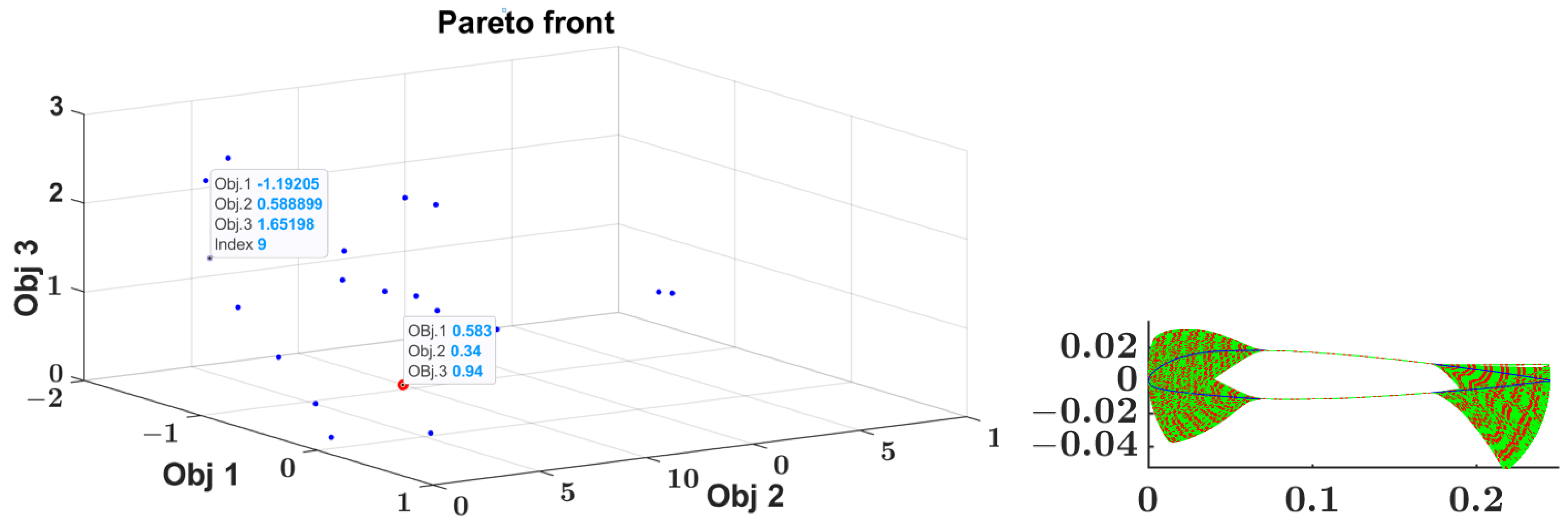
From the Pareto front output, it is possible to choose the airfoil characterized by a compromise between the Obj.1, Obj.2, and Obj.3 values following the design requirements. In the Pareto front, graphical output was also placed in the NACA 23012 position (red marker). Table 16 reports the aerodynamic and geometric properties of the initial airfoil and the chosen one from the Pareto front characterized by higher circulation and aerodynamic efficiency, as shown in Figure 36.
The aerodynamic improvement is achieved against an increase in aerodynamic drag and moment.
After the LE and TE global morphing, the airfoil was optimized considering its skin deformation always by the MATLAB gamultiobj genetic algorithm and CFD Xfoil 6.99 solver and for sections 1 and 3. In this case, the involved variables are the SFps ad the InCPs of the segments 1,3,4,6.
A Pareto front of the following three objective functions was evaluated at the same α = 4°, Re = 2.0394 × 10⁶ aerodynamic conditions:
Obj . 1 :   ( E G B E c u r r e n t ) k 1             Obj . 2 :   c m k 2             Obj . 3 :   Γ c u r r e n t Γ G B k 3
where: k 1 = 10 ;   k 2 = k 3 = 100 ;
  • E G B = aerodynamic efficiency resulting from global morphing optimization = 74.39
  • E c u r r e n t = aerodynamic efficiency of the current airfoil
  • Γ G B = airfoil circulation resulting from global morphing optimization = 1.192
  • Γ c u r r e n t = airfoil circulation of the current airfoil
The third objective function is required because, we are looking for an airfoil with improved efficiency but with the same circulation (tolerance of 1 × 10⁻³).
The three objective functions do not consider the airfoil chord because it is constant. After all, there is no LE TE rotation.
The gamultiobj options setting is options = optimoptions(@gamultiobj, ‘PlotFcn’, ‘gaplotpareto’, ‘PopulationSize’, 600, ‘MaxGenerations’,20, ‘PopulationType’, ‘doubleVector’), with a population size of 600 and 20 generations.
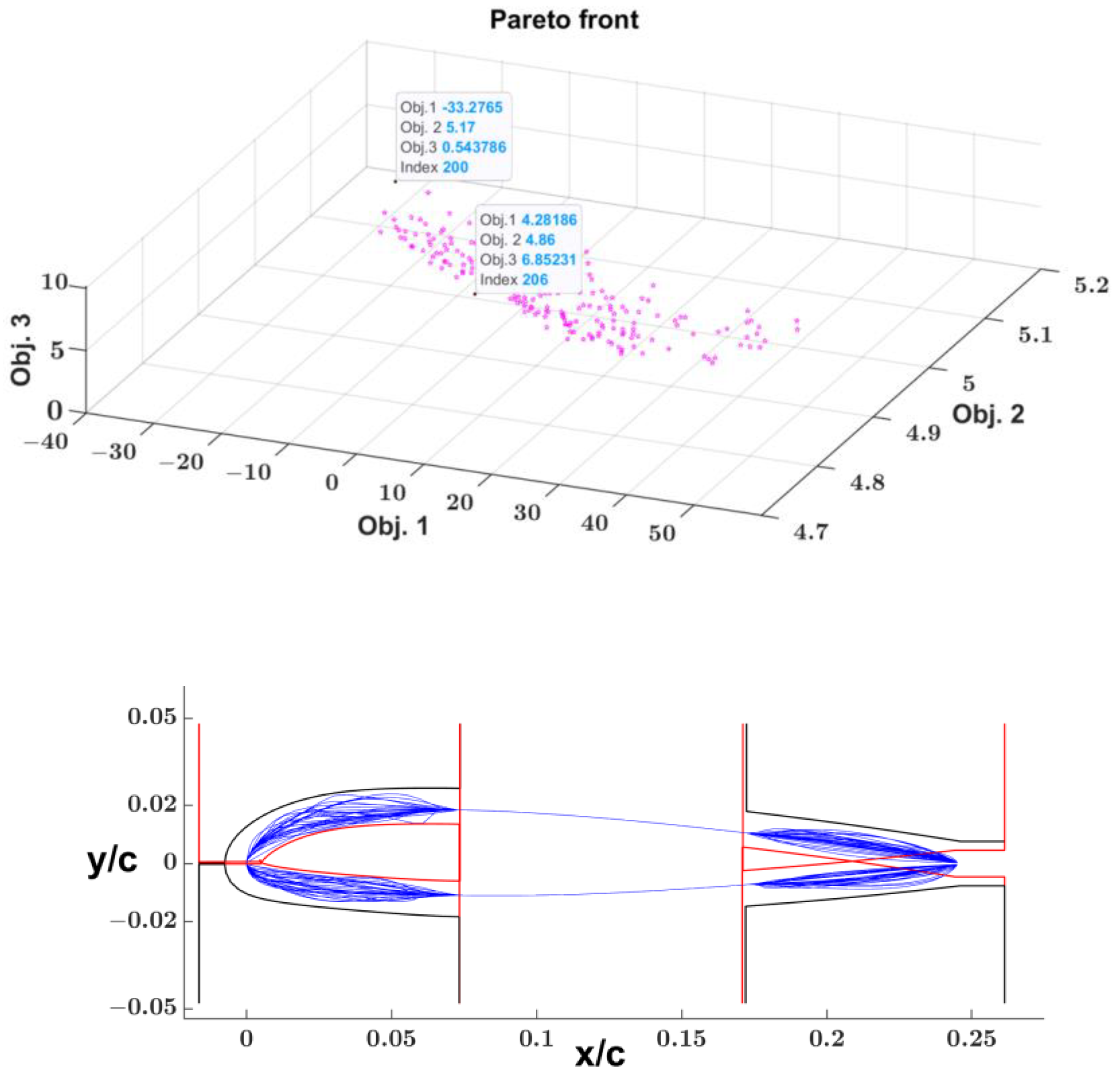
The segment-wise bounds of skin deformation are defined by offsetting the airfoil segment perimeter. The internal (red curve) and external (black curve) offsets can be adjusted by the user, as shown in Figure 37. The morphed skin is constrained inside these geometrical offset bounds.
Figure 38 represents the evaluated Pareto front skin optimization where the zero value on the obj.1 axis represents the equality of the aerodynamic efficiency between the global and skin-morphed airfoil. The obj.1 negative values represent airfoils with improved E.
Table 17 reports the comparison between the aerodynamic/geometric properties of the not-deformed NACA2312 and the global and local morphed one. The one with the highest E value and a circulation close to the global morphed with a tolerance of 1 × 10⁻³ has been chosen for the skin-morphed airfoil.
From Table 17, it is possible to assess the percentage increase in efficiency:
  • from NACA 23012 to global morphed airfoil: 18.19%
  • from global morphed airfoil to skin morphed: 4.47%
This amounts to a total increase in aerodynamic efficiency of 22.66 %.
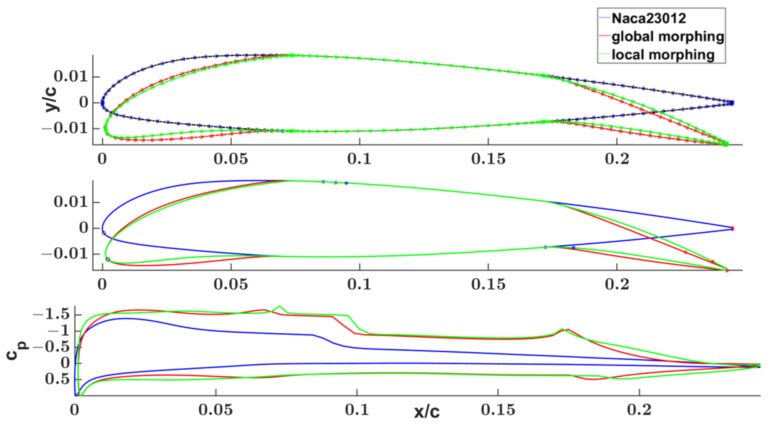
Figure 39 shows the geometry and pressure coefficient distribution both for the initial undeformed NACA 23012 airfoil and for its morphed one after the global and local design optimization process.

5. Conclusions

The results of the geometric and aerodynamic comparison, between the input airfoils and related model-based generated airfoils, show the capabilities of the new airfoil mathematical model, characterized by reduced segment parameters (SFps and InCPs):
  • to represent geometrically a wide range of 2D profile families, with the Euclidean points error distance in the order of O (10−4).
  • to generate airfoils aerodynamically equivalent to the related input 2D profile (both qualitatively and quantitatively).
Moreover, due to the presence of the B-spline segment curve as a “basic element” for the airfoil geometric description, it is possible:
  • to implement LE and TE morphing at both local and global levels (the properties of the airfoil mathematical model ensure that, for both the local and global morphing, the desired continuity boundary conditions between the neighbor segments are always satisfied);
  • to apply geometrical constraints, i.e., considering CB as a rigid/fixed section;
  • to change the relative size of each section (LE, CB, and TE) just acting on the x/c location of the partition points;
  • to evaluate the contribution of each segment/section to the aerodynamic lift and drag forces;
  • to implement CFD, structural, and FSI design optimization processes, with the opportunity to adjust the parameter topology and airfoil model complexity according to the analyst’s needs.
Moreover, taking into consideration the design optimization process:
  • Different strategies/framework can be implemented considering the opportunity to manage the variable Sfps and InCps separately.
  • The airfoil design optimization process could be implemented for defining a desired elliptical span-wise load on a LE, TE morphing rectangular wing.

Author Contributions

Conceptualization, G.T., A.C and R.P.; methodology, G.T.; software, G.T.; validation G.T.; investigation G.T., A.C. and R.P.; data curation, G.T., A.C. and R.P.; writing—original draft preparation G.T.; writing—review and editing G.T., A.C. and R.P.; supervision R.P and A.C. All authors have read and agreed to the published version of the manuscript.

Funding

This research received no external funding.

Institutional Review Board Statement

Not applicable.

Informed Consent Statement

Not applicable.

Data Availability Statement

The data presented in this study are available on request from the corresponding author.

Conflicts of Interest

The authors declare no conflict of interest.

Nomenclature

BCPsBoundary Control Points
Cthe segment vector-valued function of the u-independent variable
C′the tangent vector-valued function of the u-independent variable
C″the curvature vector-valued function of the u-independent variable
CBCentral Box
CFDComputational Fluid Dynamics
CPsControl Points
E = c l / c d Aerodynamic efficiency
InCPsInterior Control Points
LELeading-Edge
NURBSNon-Uniform Rational B-Spline
SFScale Factor
SFpsScale Factor Parameters
TETrailing-Edge
UNRBS Uniform Non-Rational B-spline

References

  1. Salunke, N.P.; Juned Ahamad, R.A.; Channiwala, S.A. Airfoil Parameterization Techniques: A Review. Am. J. Mech. Eng. 2014, 2, 99–102. [Google Scholar] [CrossRef]
  2. Song, W.; Keane, A.J. A Study of Shape Parameterisation Methods for Airfoil Optimisation. In Proceedings of the 10th AIAA/ISSMO Multidisciplinary Analysis and Optimization Conference, Albany, NY, USA, 30 August–1 September 2004. [Google Scholar] [CrossRef]
  3. Lépine, J.; Guibault, F.; Trépanier, J.-Y. Optimized Nonuniform Rational B-Spline Geometrica Representation for Aerodynamic Design of Wings. AIAA J. 2001, 39, 2033–2041. [Google Scholar] [CrossRef]
  4. Hilbig, R.; Szodruch, J. The Intelligent Wing—Aerodynamic Developments for Future Transport Aircraft. In Proceedings of the 27th Aerospace Sciences Meeting, Reno, NV, USA, 9–12 January 1989. [Google Scholar] [CrossRef]
  5. Venkataraman, P. A new procedure for airfoil definition. In Proceedings of the 13th Applied Aerodynamics Conference, San Diego, CA, USA, 19–22 June 1995; Volume 10. [Google Scholar] [CrossRef]
  6. Documentation—MATLAB & Simulink—MathWorks Italia. Available online: https://it.mathworks.com/help/ (accessed on 3 March 2022).
  7. Xfoil Subsonic Airfoil Development System. Available online: https://web.mit.edu/drela/Public/web/xfoil/ (accessed on 8 June 2022).
  8. Spink, M.; Claxton, D.; de Falco, C.; Vazquez, R. Nurbs 1.4.3. Collection of Routines for the Creation, and Manipulation of Non-Uniform Rational B-Splines (NURBS), Based on the NURBS Toolbox. 2021. Available online: https://gnu-octave.github.io/packages/nurbs/ (accessed on 11 April 2022).
  9. UIUC Applied Aerodynamics Group. Available online: https://m-selig.ae.illinois.edu/ (accessed on 18 May 2022).
  10. UIUC Airfoil Coordinates Database. Available online: https://m-selig.ae.illinois.edu/ads/coord_database.html (accessed on 18 May 2022).
  11. Abbot, I.H.; Doenhoff, A.E.V. Theory of Wing Sections; Dover: New York, NY, USA, 1985. [Google Scholar]
  12. Drela, M.; Youngren, H. xfoil_doc. 2001. Available online: http://web.mit.edu/aeroutil_v1.0/xfoil_doc.txt (accessed on 8 June 2022).
  13. Piegel, L.; Tiller, W. The NURBS Books, 2nd ed.; Springer: Berlin, Germany, 1997. [Google Scholar]
  14. Buosi, D. Development of a Parametric Tool for Shape Manipulation and Fluid Dynamics Optimization of a UHBR Engine Nacelle. Bachelor’s Thesis, University of Padova, Padua, Italy, 2019. [Google Scholar]
  15. Safari, A.; Lemu, H.G. Optimum NURBS curve fitting for geometry parameterization of gas turbine blades’ sections: Part I—evolutionary optimization techniques, in ASME 2012. In Proceedings of the International Mechanical Engineering Congress, ASME, Houston, TX, USA, 9–15 November 2012; p. 7. [Google Scholar] [CrossRef]
  16. Safari, A.; Lemu, H.G. Optimum NURBS curve fitting for geometry parameterization of gas turbine blades’ sections: Part II: Swarm intelligence techniques, in ASME 2012. In Proceedings of the International Mechanical Engineering Congress & Exposition, Houston, TX, USA, 9–15 November 2012; p. 6. [Google Scholar] [CrossRef]
  17. Safari, A.; Lemu, H.G.; Assadi, M.A.; Lemu, H.G.; Assadi, M. A novel combination of adaptive tools for turbomachinery airfoil shape optimization using a real-coded genetic algorithm. In ASME Turbo Expo 2013, Proceedings of the Turbine Technical Conference and Exposition, ASME, San Antonio, TX, USA, 3–7 June 2013; American Society of Mechanical Engineers: New York, NY, USA, 2013. [Google Scholar] [CrossRef]
  18. Deb, K. Multi-Objective Optimization Using Evolutionary Algorithms; John Wiley & Sons, Ltd.: Hoboken, NJ, USA, 2001. [Google Scholar]
  19. Branke, J.; Deb, K.; Miettinen, K.; Słowìnskì, R. Multiobjective Optimization Interactive and Evolutionary Approaches; Springer: Berlin, Germany, 2008. [Google Scholar]
  20. Oyama, A.; Obayashi, S.; Nakahashi, K. Fractional factorial design of genetic coding for aerodynamic optimization. In Proceedings of the 14th Computational Fluid Dynamics Conference, Norfolk, VA, USA, 1–5 November 1999; Volume 11. [Google Scholar] [CrossRef]
  21. Performing a Multiobjective Optimization Using the Genetic Algorithm. Available online: https://it.mathworks.com/help/gads/gamultiobj-plot-vectorize.html (accessed on 22 March 2022).
  22. Gamultiobj Find Pareto Front of Multiple Fitness Functions Using Genetic Algorithm. Available online: https://it.mathworks.com/help/gads/gamultiobj.html (accessed on 24 March 2022).
  23. Byrd, R.H.; Gilbert, J.C.; Nocedal, J. A trust region method based on interior point techniques for nonlinear programming. Math. Program. 2000, 37, 149–185. [Google Scholar] [CrossRef] [Green Version]
  24. Byrd, R.H.; Hribar, M.E.; Nocedal, J. An interior point algorithm for large-scale nonlinear programming. SIAM j. Optim. 1999, 24, 877–900. [Google Scholar] [CrossRef]
  25. Coleman, T.F.; Li, Y. An Interior Trust Region Approach for Nonlinear Minimization Subject to Bounds. SIAM J. Optim. 1996, 24, 418–445. [Google Scholar] [CrossRef] [Green Version]
  26. Fmincon Find Minimum of Constrained Nonlinear Multivariable Function. Available online: https://it.mathworks.com/help/optim/ug/fmincon.html (accessed on 22 March 2022).
  27. Constrained Nonlinear Optimization Algorithms. Available online: https://it.mathworks.com/help/optim/ug/constrained-nonlinear-optimization-algorithms.html (accessed on 22 March 2022).
Figure 1. Parsec method.
Designs 07 00028 g001
Figure 2. Cubic Bezier curve (red), control polygon (green).
Designs 07 00028 g002
Figure 3. BP 3333 airfoil geometry and Bezier control points defined by twelve basic aerodynamic parameters.
Designs 07 00028 g003
Figure 4. 2D airfoils mathematical model flowchart procedure.
Designs 07 00028 g004
Figure 5. Partitioned NACA 0012 airfoil, segments represented in different colors.
Designs 07 00028 g005
Figure 6. (b) Cubic B-spline curve and related basis functions (a).
Designs 07 00028 g006
Figure 7. Example of segments CPs distributions and parametric orientation, segments are represented in different colors.
Designs 07 00028 g007
Figure 8. Central Box segment 5 BCPs, InCPs & C′ (tangent), C″ (curvature) vectors with black and red colors respectively.
Designs 07 00028 g008
Figure 9. NACA 0012 SFs parameters lower and upper bounds seg.3 (upper LE, and extremities C’ (black color), C″ (red color) vectors.
Designs 07 00028 g009
Figure 10. Central NACA 0012 example of SF parameters numbers and values.
Designs 07 00028 g010
Figure 11. Segment fitting process, step1 flowchart.
Designs 07 00028 g011
Figure 13. NACA 0012 step 2 external Optimization cycle segment 5.
Designs 07 00028 g013
Figure 14. NACA 0012 Scale factors external optimization cycle segment 5 results.
Designs 07 00028 g014
Figure 15. NACA 0012 step 2 segment 5 fitting process: theta (°), 1st, 2nd derivatives.
Designs 07 00028 g015
Figure 16. NACA 0012 step 2 segment 5 CPs, objective function max Euclidean distance between curve and input points.
Designs 07 00028 g016
Figure 17. NACA 0012 input airfoil.
Designs 07 00028 g017
Figure 18. NACA 0012 input and evaluated maximum Euclidean point distance.
Designs 07 00028 g018
Figure 19. NACA 0012 input airfoil, evaluated airfoil, evaluated airfoil increased discretization (140 points) c l α , c l c d   c m c l , E α = c l α / c d α   comparison.
Designs 07 00028 g019aDesigns 07 00028 g019b
Figure 20. NACA 23012 input airfoil.
Designs 07 00028 g020
Figure 21. NACA 23012 input and evaluated maximum Euclidean point distance.
Designs 07 00028 g021
Figure 22. NACA 23012 input airfoil, evaluated airfoil, evaluated airfoil increased discretization (140 points) c l α , c l c d   c m c l , E α = c l α / c d α   comparison.
Designs 07 00028 g022
Figure 23. NREL’s 809 input airfoil.
Designs 07 00028 g023
Figure 24. NREL’s 809 input and evaluated maximum Euclidean point distance.
Designs 07 00028 g024
Figure 25. NREL’s 809 input airfoil, evaluated airfoil, evaluated airfoil increased discretization (140 points) c l α , c l c d   c m c l , E α = c l α / c d α   comparison.
Designs 07 00028 g025
Figure 26. NACA 23012 airfoil—segment Chebyshev discretization—Cp(x) at Re 3.5 × 10⁶, alfa 4°.
Designs 07 00028 g026
Figure 27. NACA 23012 normal & tangent vectors projection along the Vinf direction, and the normal to Vinf, the segments-wise contribution of pressure forces along the Vinf, and the normal to it.
Designs 07 00028 g027
Figure 28. NACA 23012 skin friction forces along Vinf and ⟂ Vinf directions—segment-wise contribution.
Designs 07 00028 g028
Figure 29. NACA 23012 Xfoil 6.99 polar results—Re 3.5 × 10⁶, alfa 4°.
Designs 07 00028 g029
Figure 30. Morphed NACA 23012 airfoil—segment Chebyshev discretization—Cp(x) at Re 3.5 × 10⁶, and α   = 4°; 4° and −15° rotations at the LE and TE, respectively.
Designs 07 00028 g030
Figure 31. Morphed NACA 23012 normal & tangent vectors projection along the Vinf direction, and the normal to Vinf, segments-wise contribution of pressure forces along the Vinf and the normal to it.
Designs 07 00028 g031
Figure 32. Morphed NACA 23012 segment-wise contribution of skin friction forces along Vinf and ⟂ Vinf directions.
Designs 07 00028 g032
Figure 33. Morphed NACA 23012 Xfoil 6.99 polar results—Re 3.5 × 10⁶, α = 4°, LE (4°) TE (−15°).
Designs 07 00028 g033
Figure 34. The scale factor for NACA 23012 airfoil.
Designs 07 00028 g034
Figure 35. NACA 23012 input airfoil, Mathematical model and discretization.
Designs 07 00028 g035
Figure 36. Objective functions Pareto front (left) (initial airfoil (redpoint)), airfoil global morphing (right).
Designs 07 00028 g036
Figure 37. NACA 23012 skin deformation segments bounds defined by the user.
Designs 07 00028 g037
Figure 38. NACA 23012 Pareto front skin optimization (left), airfoil local morphing (right).
Designs 07 00028 g038
Figure 39. NACA 23012 undeformed, global, and local morphing geometries and pressure coefficients.
Designs 07 00028 g039
Table 1. Partitioned airfoil topology.
Segment n°Preceding
Segment
Following
Segment
Joints
1621,2
2132,3
3243,4
4354,5
5465,6
6516,7
Table 2. Model parameters ensuring C0 continuity (more model flexibility).
Segment n°BC 0int.BC 1
JointContinuityCPsCPsJointContinuityCPsTot. Seg.
Parameters
11C0012C026
23C0212C0210
33C0214C0210
45C0214C0210
55C0216C0210
61C0016C026
Partial sum 86 12
Tot CPs 26
Tot parameters 52
Table 3. Model parameters ensuring C2 continuity (less model flexibility).
Segment n°BC 0int.BC 1
JointContinuityCPsCPsJointContinuityCPsTot.
Parameters
11C0012C202
23C2012C202
33C2014C202
45C2014C202
55C2016C202
61C0016C202
Partial sum 06 0
Tot CPs 6
Tot parameters 12
Table 4. Model parameters ensuring C2 continuity (less model flexibility).
Segment n°BC 0 int.BC 1
JointContinuityCPsSFCPsJointContinuityCPsSFTot.
Parameters
11C00012C2013
23C20112C2014
33C20114C2014
45C20114C2014
55C20116C2014
61C00016C2013
Partial sum 046 06
Tot parameters 22
Table 5. BCPs user-defined bounds & SF evaluated upper and lower bounds.
Seg. n°BC 0BC 1
JointCPCPSFSFJointCPCPSFSF
Xmin%Xmax%LbUbXmin%Xmax%LbUb
11----285960.15490.4243
235150.58191.6249285960.62821.8958
335150.23350.6911485990.19581.0372
455150.27470.8131485990.23030.9511
555150.31410.9511685960.29090.8149
67----685960.15490.4243
Table 6. Segment-wise evaluated SFs.
BC 0—SFsBC 1—SF
Seg. n°JointLbValueUbJointLbValueUb
11- -20.15490.25740.4243
230.58191.31101.624920.62821.65271.8958
330.23350.67770.691140.19580.82791.0372
450.27470.61930.813140.23030.53600.9511
550.31410.93320.951160.29090.68460.8149
67- -60.15490.21520.4243
Table 7. Segment-wise strategy boundary conditions implementations.
Seg.PriorityJointsContinuityBoundary DataTangent Curvature
Numerical Evaluation
121C0Input Airfoil point-
2C2Segment 2Segments 1 & 2
Tangent curvature vectorB-spline interpolation
212C2Input Airfoil pointsSegments 1 & 2
B-spline interpolation
3C2Input Airfoil pointsSegments 2 & 3
B-spline interpolation
333C2Segment 2Segments 2 & 3
Tangent curvature vectorB-spline interpolation
4C2Input Airfoil pointsSegments 3 & 4
B-spline interpolation
444C2Segment 3Segments 3 & 4
Tangent curvature vectorB-spline interpolation
5C2Segment 5Segments 4 & 5
Tangent curvature vectorB-spline interpolation
515C2Input Airfoil pointsSegments 4 & 5
B-spline interpolation
6C2Input Airfoil pointsSegments 5 & 6
B-spline interpolation
626C2Segment 5Segments 5 & 6
Tangent curvature vectorB-spline interpolation
7C0Input Airfoil points-
Table 8. New mathematical model fitting process segment-wise computation time.
Seg. N°NACA 0012
(hh:mm:ss)
NACA 23012
(hh:mm:ss)
NREL’s S089
(hh:mm:ss)
100:09:2600:08:5400:07:56
200:16:0100:14:0500:07:53
300:14:2200:13:3800:14:07
400:14:2500:06:3000:15:13
500:15:1400:16:0000:13:51
600:08:2400:09:3500:10:40
Tot01:17:5201:08:4201:09:40
Table 9. New mathematical model fitting process geometrical approximation.
Seg. N°NACA0012NACA 23012NREL’s S809
max(abs(dy))sum(abs(dy))max(abs(dy))sum(abs(dy))max(abs(dy))sum(abs(dy))
14.81 × 10−50.000294.79 × 10−50.000300.000600.00349
21.22 × 10−50.000071.94 × 10−50.000140.000330.00174
38.16 × 10−50.000749.06 × 10−50.000950.000220.00184
40.000190.001820.000620.006420.000600.00559
50.000120.000830.000110.000800.000350.00155
64.68 × 10−50.000304.79 × 10−50.000310.000600.00299
Tot 0.00405 0.00892 0.0172
Table 10. New mathematical model fitting process segment-wise computation time.
Segment N°RAE2822
(hh:mm:ss)
NACA 0406
(hh:mm:ss)
NACA 0610
(hh:mm:ss)
100:04:0900:12:5700:16:40
200:13:4600:04:1200:04:02
300:06:5800:12:3400:13:57
400:20:1400:03:3900:09:03
500:21:5300:19:4700:18:38
600:04:4000:13:1200:13:04
Timing tot01:11:4001:06:2101:15:24
Table 11. New mathematical model fitting process geometrical approximation.
Segment N°RAE2822
sum(abs(dy))
NACA 0406
sum(abs(dy))
NACA 0610
sum(abs(dy))
10.002100.002370.00267
20.000510.004350.00426
30.002340.004180.00102
40.002600.003220.00294
50.001360.002360.00137
60.002100.000960.00226
Tot0.011010.017440.01452
Table 12. Summary of different parameter methods for airfoils.
MethodParameters
Number
Parameters
Description
Numerical Basis Functions5Weights for the basis airfoil functions
B-spline interpolation34Point coordinates
Proposed method22SFs and point coordinates
Table 13. Best Approximation of target airfoils for different parameterizations.
MethodRAE2822NACA 0406NACA 0610
Numerical Basis Functions0.2217 0.05820.1595
B-spline interpolation0.1552 0.07580.1993
Proposed method0.01100.01740.0145
Table 14. NACA 23012 Xfoil 6.99 aerodynamic results segment-wise distribution (Re = 3.5 × 10⁶, α   = 4°).
clcdcdp
Xfoil output 0.57430.006010.00166
iclicfi⊥ Vinfcfi || Vinf
Segment 10.0126−0.000140.00068
Segment 20.1697−0.000240.00161
Segment 30.32180.000270.00120
Segment 40.0592−0.000130.00045
Segment 5−0.0073−0.000010.00023
Segment 60.01820.000010.00018
Tot 0.5742−0.000240.00435
cl = Σ cli + Σ (cfi ⊥ Vinf) 0.5740
cdp = cd − Σ(cfi || Vinf) 0.00166
Table 15. NACA 23012 Xfoil 6.99 aerodynamic results segments wise distribution—Re 3.5 × 10⁶, α = 4°, LE (4°) TE (−15°).
. clcdcdp
Xfoil output 1.50980.017240.01095
iclicfi⊥ Vinfcfi || Vinf
Segment 10.1106−0.000230.00062
Segment 20.4239−0.000310.00209
Segment 30.54720.000600.00246
Segment 40.1638−0.000160.00036
Segment 50.1535−0.000010.00019
Segment 60.1109−0.000170.00069
Tot 1.5099−0.000270.00640
cl = Σ cli + Σ (cfi ⊥ Vinf) 1.5096
cdp = cd – Σ(cfi || Vinf) 0.01084
Table 16. Initial and “global” morphed NCA 23012.
α = 4°, Re = 2.0394 × 10⁶NACA 23012
Initial
NACA 23013
Global Morphing
Obj.10.5831.192
Obj.20.3400.589
Obj.30.9401.652
c 0.245 m0.242 m
c c l 3.89 × 10−27.95 × 10−2
c c d 6.17 × 10−41.07 × 10−3
c 2 c m 1.7 × 10−33.00 × 10−3
c l 0.15860.329
c d 2.52 × 10−34.42 × 10−3
c m 2.84 × 10−25.13 × 10−2
E = c l / c d 62.9474.39
LE (°)08.08
TE (°)012.6
Table 17. Initial and “global” morphed NCA 23012.
α = 4°, Re = 2.0394 × 10⁶NACA 23012
Initial
NACA 23013
Global Morphing
NACA 23013
Skin Morphing
c 0.245 m0.242 m0.242 m
c c l 3.89 × 10−27.95 × 10−27.98 × 10⁻²
c c d 6.17 × 10−41.07 × 10−31.07 × 10⁻³
c 2 c m 1.7 × 10−33.00 × 10−33.03 × 10⁻³
c l 0.15860.3290.330
c d 2.52 × 10−34.42 × 10−34.42 × 10⁻³
c m 2.84 × 10−25.13 × 10−25.17 × 10⁻²
E = c l / c d 62.9474.3978.26
LE (°)08.088.08
TE (°)012.612.6
Disclaimer/Publisher’s Note: The statements, opinions and data contained in all publications are solely those of the individual author(s) and contributor(s) and not of MDPI and/or the editor(s). MDPI and/or the editor(s) disclaim responsibility for any injury to people or property resulting from any ideas, methods, instructions or products referred to in the content.