Estimating the Optimum Weight for Latticed Power-Transmission Towers Using Different (AI) Techniques

Abstract

The recent expansion of power-distribution networks has motivated many researchers to study how to minimize the costs of such projects. Although transmission towers present one of the main items in the network that greatly affect the project budget, there are no clear criteria or recommendations to select the optimum bracing system that minimizes the tower weight. This research presents recommendations to select the optimum configurations for latticed power-transmission towers, segment by segment, for certain loads, as well as the aspect ratio. The research started by generating a database with different segment configurations and their weights, and then three of the most famous AI techniques (GP, ANN and EPR) were used to generate models to calculate the weights of the segments. Studying these models led to the conclusion that K-shape bracing is better that X-shape bracing for segments with aspect ratios (H/B) less than 1.0. The generated models and conclusions were verified by using existing tower designs.

1. Introduction

Latticed power-transmission towers are one of the main items in any power-distribution network. They cost about 35–45% of the total cost of the overhead transmission line (F. Kiessling et al., 2003) [1]. This fact has motivated many researchers to minimize and optimize the costs of this important item. Both Shea, K. and Smith, I.F.C, 2006 [2] and Huiyong Guo and Zhengliang Li, 2011 [3] carried out studies to improve tower designs using topology optimization, while I. Couceiro et al., 2016 [4] used the simulated annealing algorithm to optimize lattice steel transmission towers. Huiyong Guo and Zhengliang Li, 2009 [5], Abdullah and Taysi, 2012 [6], Sanah Rose Sony and Airin M. G., 2016 [7], J. Premalatha et al., 2017 [8] and Bharat Koner et al., 2018 [9] applied the genetic algorithm to optimize the design of lattice steel transmission towers. Siamak Talatahari et al., 2012 [10], R. Nagavinothini and C. Subramanian, 2015 [11] and Li et al., 2015 [12] tried to achieve the optimum design of transmission towers by using the firefly algorithm, PSO algorithm and ant-colony-optimization algorithm, respectively. Ebid et al., 2021 [13] and El-Aghoury et al., 2022 [14] presented optimization models to design steel members using GRG and ANN techniques, respectively. Gencturk et al., 2012 [15] used the “Taboo Algorithm” to optimize the design of lattice wind-turbine towers, while Hosseini et al., 2021 [16] implemented the “Adaptive Neuro Fuzzy Inference System with Biogeography Based Optimization” technique (ANFIS-BBO) to optimize the size, shape and design of transmission tower panels. Nguyen et al., 2022 [17] used the “Differential Evolution and Machine Learning Classification” (DE-MLC) technique to minimize the weights of steel lattice transmission towers. Finally, Ebid, 2022 [18] presents a GP model to estimate the total weight of a steel lattice transmission tower based on actual database collected from several tender documents in the middle east zone.

Artificial intelligence (AI) has been used in engineering since the 1980s, and its applications have become very acceptable today. Genetic programming (GP) is one of the famous AI techniques; it was invented by Cramer (1985) [19] and developed by Koza (1992) [20]. Today, GP is an umbrella for many subtechniques, all of which were developed on the basis of the same concepts as GP, such as evolutionary polynomial regression (EPR), the gene expression programming technique (GEP), Cartesian genetic programming (CGP), linear genetic programming (LGP), meta-genetic programming (MGP) and multigene genetic programming (MGGP), in addition to the classic GP.

The main concept of GP is to apply the genetic-algorithm (GA) technique to mathematical formulas. The GA technique is one of the earliest AI techniques. It mimics Darwin’s evolution theory by generating a number of random solutions for the considered problem, testing the fitness of each solution, selecting the most fitting solutions and erasing the rest; then, the surviving solutions are mixed to create the next generation of solutions using one of the crossover techniques, and the cycle goes on until the desired fitting level is achieved. In GP, the mathematical formulas have to be coded in binary-tree form and then converted into the genetic algorithm in order to apply GA operators on them. Figure 1 explains the concepts of binary tree and genetic form.

2. Objective

Although many researchers have addressed this topic before, none of them have introduced a certain procedure, or even guidelines, to choose geometrical configurations that lead to minimum tower weights.

The main concept of this research is based on the fact that latticed power-transmission towers usually consist of a number of segments, which are erected one over top of the other, starting from the biggest at the bottom and ending with the smallest at the top. Each segment is a 3D vertical cantilever truss structure, fixed at the bottom in the lower segment (or in the foundation), and loaded at the top from the upper segment (or from cross arms). Accordingly, optimizing the weight of each individual segment leads to optimizing the weight of the whole tower. Based on the previous concept, the aim of this research is to present an AI model to estimate the optimum weights of individual tower segments. Based on the developed models, guidelines are recommended to select the optimum segment configurations to minimize the weight. Applying these guidelines to the design of individual segments is a way to optimize the weight of the whole tower.

3. Methodology

The research plan was divided into two phases: the first phase carried out a parametric study of more than 500 individual segments with different geometrical configurations and loading conditions, which were designed according to ASCE manuals and reports on engineering practice (No. 52 “Guide for design of steel transmission towers”). In the second phase, the genetic-programming technique was applied on the results of the parametric study to generate the best-fitting mathematical formula that correlated the individual segment geometrical configurations and loading conditions with its optimum weight. The following paragraphs describe the research plan in detail. Then, the generated formula was studied to extract general guidelines and recommendations to achieve the minimum weights of the tower segments.

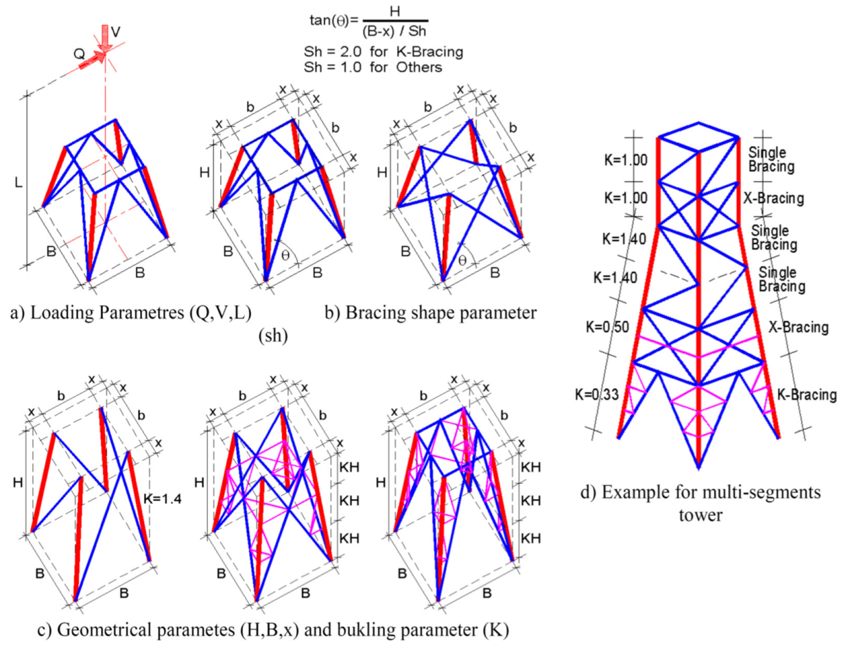
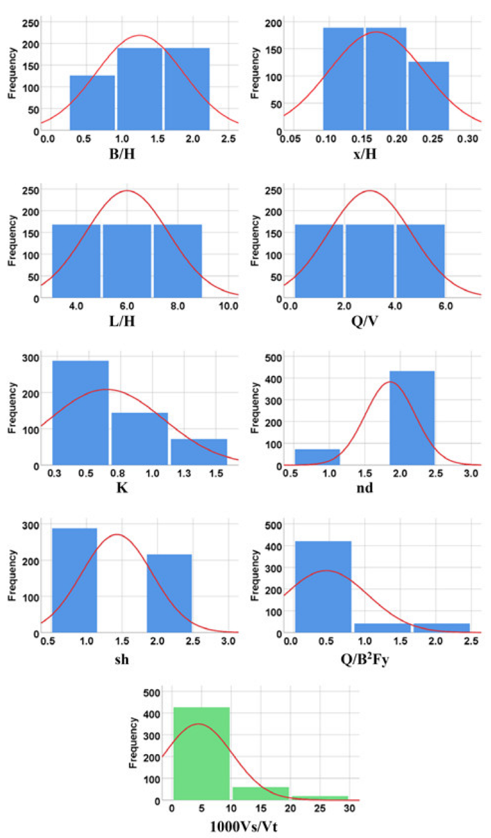
3.1. Phase I: The Parametric Study

This parametric study aimed to generate the required database for the next phase. The study started out by determining the parameters that affect the segment weight, which could be classified into geometrical and loading parameters. The geometrical parameters were the segment height (H), bottom width (B), leg-slope angle (α), diagonal shape (single diagonal, X-diagonals and K-diagonals), and the arrangement of the subdividers. In order to quantify these parameters and avoid the use of angles, the leg-slope angle (α) was replaced by the length (x), where tan(α) = x/H. The diagonal shape was presented by two parameters: the number of diagonals per face (nd), and the diagonal-slope angle (θ); again, the diagonal-slope angle (θ) was replaced by the shape factor (sh), where tan(θ) = (H.sh)/(B-x).

Finally, the arrangement of the subdividers was presented by the bulking coefficient (K). The loading parameters were the vertical load (V), lateral load (Q) and the vertical distance between the applying point of the lateral load and the segment base (L). Figure 2 shows both the geometrical and loading parameters.

The next step was to determine the value range of each parameter, as shown in

Table 1. Value ranges of the parametric study.

Parameter	Symbol	Unit	Values
Segment height	(H)	(m)	4.0
Bottom width	(B)	(m)	2.0, 4.0, 8.0
(x) distance	(x)	(m)	0.35, 0.70, 1.05
(L) distance	(L)	(m)	16.0, 24.0, 32.0
Vertical load	(V)	(ton)	6.0
Lateral load	(Q)	(ton)	6.0, 18.0, 30.0
Buckling coefficient	(K)	-	1.4, 1.0, 0.33, 0.2
Shape factor	(sh)	-	1.0, 2.0

; then, 504 combinations of these values were generated. Each combination presents a segment with a different geometrical configuration and loading condition.

In order to design and calculate the weight of the generated segments, the following assumptions were considered:

• The plan of the tower is square;
• All legs have the same cross section;
• All diagonals have the same cross section;
• All cross-frame members have the same cross section;
• All subdivide members have the same cross section;
• Cross sections of all members are single angles;
• Only equal angles with size to thickness (a/t) equal to 10 are used;
• Minimum allowed cross sections are L40 × 40 × 4 for subdividers, and L50 × 50 × 5 for other members;
• All members have a minimum yield stress of 3.6 t/cm² (36,000 t/m²);
• Since the leg slope ranged between 5° and 15°, all member lengths are calculated as in the vertical plane;
• The subdividers divide both legs and diagonals into equal lengths;
• The lateral load is considered in one direction;
• In the case of X-diagonals and K-diagonals, both diagonal members are active, and no post-buckling behavior is allowed;
• The maximum allowable values for the buckling factor (λ = KL/r) are 150, 200 and 250 for legs, diagonals and subdividers, respectively.

3.2. Phase II: Artificial Intelligence (AI) Models

The aim of this phase was to correlate the calculated segment weight with its corresponding geometrical and loading parameters using different AI techniques, which were, namely, genetic programming (GP), artificial neural network (ANN) and evolutionary polynomial regression (EPR). The first step to apply these techniques is to prepare a database in a proper format by converting the absolute values of the parameters into dimensionless ones; hence, all the lengths were divided by the segment height (H), the vertical load was related to the lateral load and, finally, the absolute value of the lateral load was replaced by the dimensionless parameter (Q/B²Fy), where (Fy) is the yield stress of the used steel. Accordingly, the considered eight dimensionless parameters are: B/H, x/H, L/H, Q/V, K, nd, sh and Q/B²Fy. Similarly, the absolute calculated segment weight was presented by a dimensionless value (1000 Vs/Vt), where Vs is the summation of all steel members’ volumes, and Vt is the maximum total volume of the segment (B²H). The 504 database records were divided into two groups: a training group of 354 records, and a validation group of 150 records. The statistical proprieties of the database items and their correlations are summarized in

Table 2. Pearson correlation matrix.

	B/H	x/H	L/H	Q/V	K	nd	sh	Q/B2fy	1000 Vs/Vt
B/H	1.00
x/H	0.19	1.00
L/H	0.00	0.00	1.00
Q/V	0.00	0.00	0.00	1.00
K	0.00	0.00	0.00	0.00	1.00
nd	0.00	0.00	0.00	0.00	−0.69	1.00
sh	0.00	0.00	0.00	0.00	−0.24	0.35	1.00
Q/B2fy	−0.67	−0.21	0.00	0.42	0.00	0.00	0.00	1.00
1000 Vs/Vt	−0.66	−0.23	0.08	0.23	0.27	−0.20	−0.01	0.89	1.00

and

Table 3. Statistical proprieties of database parameters.

	B/H	x/H	L/H	Q/V	K	nd	sh	Q/B2fy	1000 Vs/Vt
Training set
Min.	0.50	0.09	4.00	1.00	0.20	1.00	1.00	0.03	0.32
Max.	2.00	0.26	8.00	5.00	1.40	2.00	2.00	2.08	28.15
Avg.	1.25	0.17	5.97	2.97	0.78	1.80	1.19	0.46	4.82
SD	0.61	0.07	1.63	1.63	0.45	0.40	0.39	0.59	6.00
VAR	0.49	0.40	0.27	0.55	0.58	0.22	0.33	1.28	1.24
Validation set
Min.	0.50	0.09	4.00	1.00	0.20	2.00	2.00	0.03	0.35
Max.	2.00	0.26	8.00	5.00	1.00	2.00	2.00	2.08	28.70
Avg.	1.26	0.17	6.08	3.08	0.30	2.00	2.00	0.46	3.62
SD	0.61	0.07	1.65	1.65	0.16	0.00	0.00	0.59	4.96
VAR	0.49	0.40	0.27	0.53	0.53	0.00	0.00	1.28	1.37

, while Figure 3 graphically presents the input and output datasets (using histograms), which provide a quick visual idea as to the the range, distribution, mean and median of each parameter, in addition to the traditional tabulated format presented in Table 2. After predicting the 1000 Vs/Vt values using the AI techniques, the segment weight could be calculated as follows:

$$Ws \left(kg\right)=\left(\frac{1000 Vs}{Vt}\right)\left({\mathsf{\gamma }\mathrm{s}\mathrm{B}}^2\mathrm{H}\right)$$

(1)

where (γs) is the steel density (8.0 t/m³).

The following section discusses the results of each model. The accuracies of the developed models were evaluated by comparing the SSE between the predicted and calculated 1000 Vs/Vt values. The results of all developed models are summarized at the end of Section 4.

4. Research Results

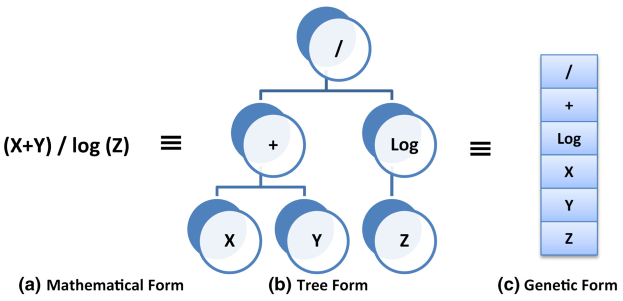
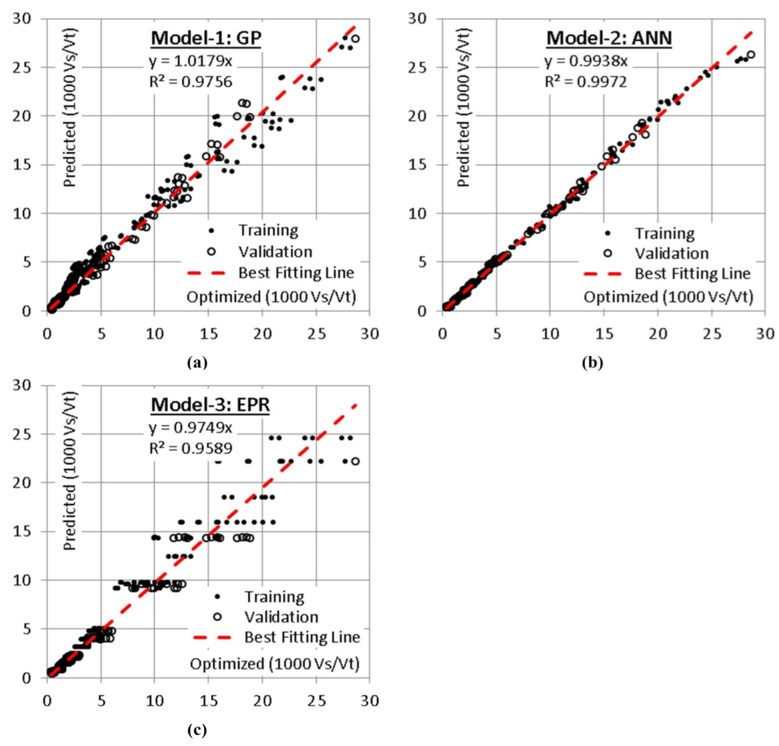
4.1. Model 1 Using GP

The developed GP model started with one level of complexity and settled at five levels of complexity. The population size, survivor size and number of generations were 100,000, 30,000 and 200, respectively. Equation (2) presents the output formulas for 1000 Vs/Vt, while Figure 5a shows its fitness. The average error % of this equation is 16.6 %, while the R² value is 0.976. The estimated segment weight could be calculated using Equation (1):

$$\frac{1000 Vs}{Vt}=\frac{Q}{ B^{2}Fy}\frac{L}{H}+K\frac{H}{B} \left[1+{\left(\frac{H}{B}\right)}^{sh}\right]-\frac{x}{H}-ln\left(n_d\right)+{\left(\frac{Q K}{ B^{2}Fy}\right)}^{\frac{B}{H}\frac{Q }{ B^{2}Fy}}$$

(2)

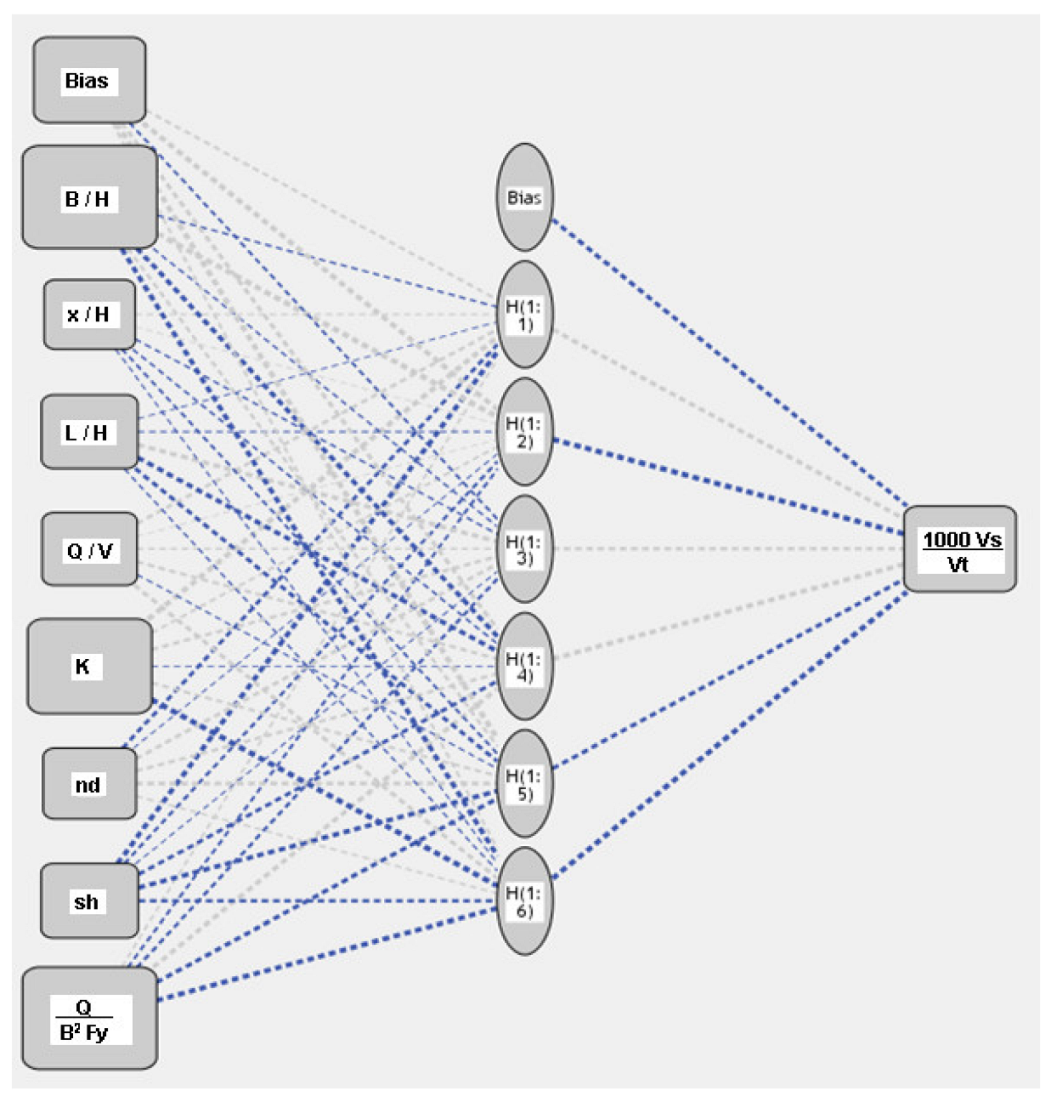
4.2. Model 2 Using ANN

A back-propagation ANN with two hidden layers and an (Hyper Tan) activation function was used to predict the same 1000 Vs/Vt values. The used network layout and its connation weights are illustrated in Figure 4 and

Table 4. Connection weights for the developed ANN.

		Hidden Layer 1						Output Layer
		H(1:1)	H(1:2)	H(1:3)	H(1:4)	H(1:5)	H(1:6)	1000 VsVt
Input Layer	(Bias)	0.215	0.660	−0.177	0.353	0.779	0.206
	B/H	−0.090	1.165	−0.082	−0.435	0.238	−0.495
	x/H	0.075	0.013	−0.090	−0.092	−0.171	−0.044
	L/H	−0.016	−0.033	0.415	−0.432	−0.340	−0.082
	Q/V	0.274	0.008	0.158	0.256	−0.068	0.345
	K	0.662	0.186	0.271	−0.015	0.222	−1.012
	nd	−0.295	−0.018	0.289	0.266	0.369	0.098
	sh	−0.509	−0.220	−0.023	−0.320	−0.471	−0.281
	Q/B2fy	0.116	−0.205	−0.230	0.401	−0.373	−0.615
Hidden Layer 1	(Bias)							−0.374
	H(1:1)							0.381
	H(1:2)							−1.016
	H(1:3)							0.327
	H(1:4)							0.524
	H(1:5)							−0.362
	H(1:6)							−0.732

. The average error % of this model is 6.8%, and the corresponding (R²) value is 0.997. The relation between the calculated and predicted values is shown in Figure 5b. The estimated segment weight could be calculated using Equation (1).

4.3. Model 3 Using EPR

Finally, the developed EPR model was limited to the quadrilateral level; for eight inputs, there are 495 possible terms (330 + 120 + 36 + 8 + 1 = 495), as follows:

$${\displaystyle \sum }_{i=1}^{i=8}{\displaystyle \sum }_{j=1}^{j=8}{\displaystyle \sum }_{k=1}^{k=8}{\displaystyle \sum }_{l=1}^{l=8}{X}_i.X_j.X_k.X_l+{\displaystyle \sum }_{i=1}^{i=8}{\displaystyle \sum }_{j=1}^{j=8}{\displaystyle \sum }_{k=1}^{k=8}{X}_i.X_j.X_k+{\displaystyle \sum }_{i=1}^{i=8}{\displaystyle \sum }_{j=1}^{j=8}{X}_i.X_j+{\displaystyle \sum }_{i=1}^{i=8}{X}_i+C$$

The GA technique was applied on these 495 terms to select the six most effective terms to predict the 1000 Vs/Vt values. The output is illustrated in Equation (3), and its fitness is shown in Figure 5c. The average error % and R² value were 25.8% and 0.959 for the total datasets, respectively. The estimated segment weight could be calculated using Equation (1).

$$\frac{1000\mathrm{Vs}}{\mathrm{Vt}}=\frac{\mathrm{Q}}{{\mathrm{B}}^2.\mathrm{fy}}\left[\frac{1.95\mathrm{H}.\mathrm{K}}{\mathrm{B}}+\frac{0.224\mathrm{H}}{\mathrm{B}.\mathrm{K}}+\frac{0.789\mathrm{H}.\mathrm{nd}}{\mathrm{B}}+\frac{14.95\mathrm{V}.\mathrm{K}}{\mathrm{Q}}\right]+\frac{0.55\mathrm{B}.\mathrm{K}}{\mathrm{H}.\mathrm{nd}}+0.213$$

(3)

Finally,

Table 5. Accuracies of developed models.

Technique	Developed Equation	(MSE)	(MSE)	Error %	R2
GP	Equation (2)	0.917	424	16.6	0.976
ANN	Figure 4	0.303	46	6.8	0.997
EPR	Equation (3)	1.154	671	25.8	0.959

summarizes the accuracies of developed models.

5. Dissection

A study of the three developed models showed that the ANN model is not only the most accurate one (93.2%), but also the most complicated. Due to its complexity, it cannot be manually used; however, it is recommended as software. The summation of the absolute weights of each neuron in the input layer is a good indicator of the importance of its parameter. Accordingly, the most effective parameters were Q/B²Fy, B/H and K, while the other parameters had minor effects on the weight of the segment.

Conversely, the EPR model had the lowest level of accuracy (74.2%), as indicated by the scattered points in Figure 5c. Although it presents a simple closed-form equation, it is not recommended due to its level of accuracy.

Finally, the GP model introduces a simple formula with reasonable accuracy (83.4%), as shown in Equation (2). This equation could be simplified to Equation (4) by using the following substitutions:

• Segment volume (Vt = B²H);
• Overturning moment at segment base (M = Q.L);
• Segment aspect ratio (A = H/B);
• Yield stress of steel (Fy = 3.6 t/cm² = 36,000 t/m²):

$$1000Vs=0.28M+Vt\left[KA\left(1+A^{sh}\right)-ln\left(n_d\right)-\frac{x}{H}\right]+Vt{\left(\frac{QK}{3.6B^2}\right)}^{\frac{Q}{3.6\mathrm{H}\mathrm{B}}}$$

(4)

The segment weight could be calculated as shown in Equation (1); hence:

$$Ws\left(kg\right)=2.25M+8Vt\left[KA\left(1+A^{sh}\right)-ln\left(n_d\right)-\frac{x}{H}\right]+8Vt{\left(\frac{QK}{3.6B^2}\right)}^{\frac{Q}{3.6\mathrm{H}\mathrm{B}}}$$

(5)

where Q is in tons, M is in m.t and all lengths are in meters.

Studying Equation (5) indicates the following:

• The term $\left(1+A^{sh}\right)$ in Equation (5) is minimized when A < 1.0 and sh = 2, and when A > 1.0 and sh = 1. This indicates that K-bracing is favorable when the aspect ratio (A) is less than 1.0, while X-bracing is favorable for an A greater than 1.0;
• In order to keep the diagonal angle in the optimum zone (from 30° to 60°), the segment aspect ratio (A) should be between 0.5 and 2.0;
• The term $-ln\left(n_d\right)$ in Equation (5) indicates that using a two-member bracing system is always more economical than using a one-member bracing system;
• The buckling factor (K) appeared in two positive terms: $KA\left(1+A^{sh}\right)$ and ${\left(\frac{QK}{3.6B^2}\right)}^{\frac{Q}{3.6\mathrm{H}\mathrm{B}}}$. This means that decreasing the K factor decreases the segment weight. However, decreasing the K value to below 10 a/H, which corresponds to (λ = 50), will not significantly affect the segment weight. Conversely, using a K value higher than 20 a/H, which corresponds to (λ = 100), eliminates the advantage of using high-strength steel due to the Euler buckling;
• The term ${\left(\frac{QK}{3.6B^2}\right)}^{\frac{Q}{3.6\mathrm{H}\mathrm{B}}}$ tends to zero for large segments, which indicates that it presents the effect of not using subdividers in small segments (using large K values) when increasing their weights;
• Finally, the term $-\frac{x}{H}$ in Equation (5) indicates that increasing the base width of the segments reduces their weights, but this is limited within the optimum range of the aspect ratio (A) (which lays between 0.5 and 2.0). The practical leg slope in most prefabricated latticed power-transmission towers ranges between 5° and 15°.

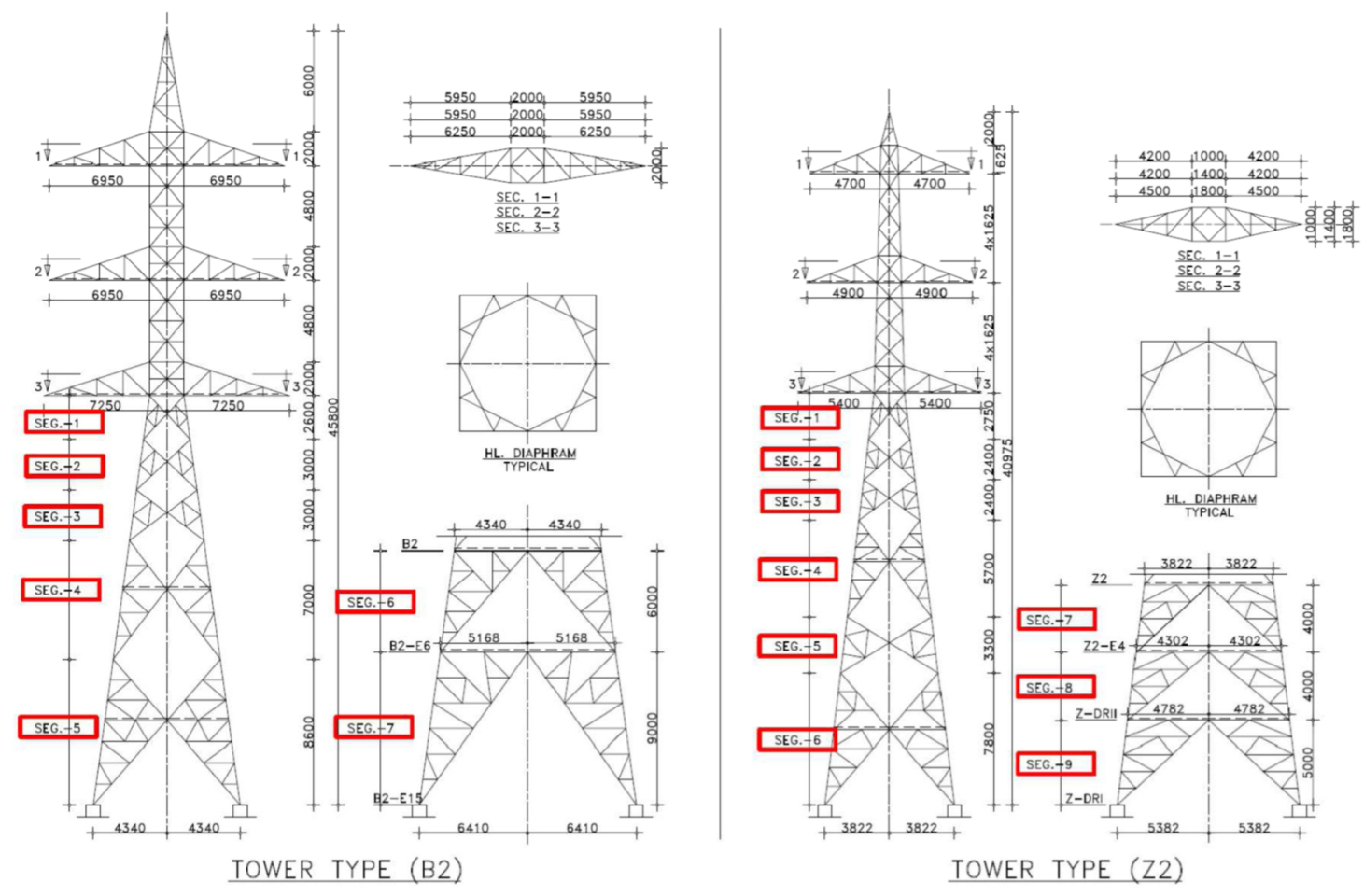
6. Verification

In order to assure the validity of Equation (3) and the ANN model, two preoptimized prefabricated models of latticed towers (B2 and Z2) were used. Z2 is a 360 m-spanning 220 KV double-circuit double-conductor suspended tower, while B2 is a 360 m-spanning 220 KV double-circuit triple-conductor suspended tower. Each one of them consists of various numbers of segments with different heights, aspect ratios and diagonal shapes. Line diagrams of both towers are presented in Figure 6.

It can be noted from

Table 6. Summary of the verification results.

Seg.	H	B	x	Q	L	K	nd	sh	Ws act	Ws Equation (5)	Ws ANN
ID	(m)	(m)	(m)	(t)	(m)	(-)	(-)	(-)	(kg)	(kg)	(kg)
Tower Type (Z2)
1	2.75	2.46	0.33	18.2	9.55	0.25	2.00	1.00	380	384	391
2	2.40	3.04	0.29	18.4	11.83	0.25	2.00	1.00	400	380	388
3	2.40	3.61	0.29	18.6	14.06	0.25	2.00	1.00	500	475	535
4	5.70	4.98	0.68	19.3	19.04	0.16	2.00	1.00	930	902	930
5	3.30	5.77	0.40	19.8	21.80	0.33	2.00	1.00	950	1017	931
6	7.80	7.64	0.94	21.3	27.52	0.14	2.00	1.00	1750	1785	1855
7	4.00	8.60	0.48	22.1	30.30	0.25	2.00	2.00	1344	1304	1277
8	4.00	9.56	0.48	23.1	32.88	0.25	2.00	2.00	1461	1373	1359
9	5.00	10.76	0.60	24.4	35.79	0.20	2.00	2.00	2022	2062	2123
							Total		9737	8533	9789
Tower Type (B2)
1	2.60	2.72	0.36	26.2	9.94	0.25	2.00	1.00	532	559	548
2	3.00	3.55	0.42	26.4	12.81	0.25	2.00	1.00	639	698	620
3	3.00	4.38	0.42	26.8	15.62	0.25	2.00	1.00	683	802	703
4	7.00	6.32	0.97	27.9	21.72	0.20	2.00	1.00	1758	1797	1758
5	8.60	8.70	1.19	29.7	28.42	0.14	2.00	1.00	2355	2262	2308
6	6.00	10.37	0.84	31.3	32.71	0.20	2.00	2.00	2091	1673	2091
7	9.00	12.86	1.25	34.2	38.19	0.16	2.00	2.00	2985	3084	3134
							Total		11,043	10,875	11,162

that the lateral load (Q) increased for lower segments due to the wind load on the tower body, and consequently, the length (L) was calculated by dividing the overturning moment (M) by the lateral load (Q).

The weight of each segment and the total weights of the towers were compared with the calculated values from Equation (5) and the ANN model, as summarized in Table 6. The results showed almost the same level of prediction accuracy as the generated database.

7. Conclusions

This research presents three models using three AI techniques: GP, ANN and EPR, to predict the optimum weight of a tower segment based on its geometrical configurations and loading conditions. The research results can be concluded in the following points:

• The developed ANN model is the most accurate model, with an average error of 6.8%; however, it is too complicated to be applied manually and it cannot be used to extract design guidelines;
• The EPR model has the lowest level of accuracy, with an average error of 25.8%, and accordingly it is not recommended;
• The reasonable accuracy of the GP formula (error: 16.6%), in addition to its ability to be applied manually, makes it the best choice for further analysis to extract design guidelines to minimize the segment weight, as follows:

  o

  K-bracing is favorable when the aspect ratio (A) is less than 1.0, while X-bracing is favorable for an A more than 1.0;

  o

  The segment aspect ratio (A) should be between 0.5 and 2.0;

  o

  A double-member bracing system is always more economical than a single-member bracing system;

  o

  The distance between the subdividers should be between 10 and 20 times the leg-angle size;

  o

  The practical leg slope is between 5° and 15°, which corresponds to an x/H value between 0.10 and 0.25. However, the selected value should comply with the optimum range of the aspect ratio (A), which is between 0.5 and 2.0;

• The accuracies of both the GP and ANN models were verified using two types of preoptimized tower segments;
• As with any other regression technique, the developed models are valid within the considered range of the parameter values; beyond this range, the prediction accuracy should be verified;
• Further studies may be carried out to optimize the design of guided and communication towers using the same technique.

References

- Kiessling, F.; Nefzger, P.; Nolasco, J.E.; Kaintzyk, U. Overhead Power Lines Planning, Design, Construction; Springer: Berlin/Heidelberg, Germany; New York, NY, USA, 2003; ISBN 3-540-00297-9. [Google Scholar]
- Shea, K.; Smith, I.F.C. Improving Full-Scale Transmission Tower Design through Topology and Shape Optimization. J. Struct. Eng. 2006, 132, 781–790. [Google Scholar] [CrossRef] [Green Version]
- Guo, H.Y.; Li, Z.L. Structural topology optimization of high-voltage transmission tower with discrete variables. Struct. Multidisc. Optim. 2011, 43, 851–861. [Google Scholar] [CrossRef]
- Couceiro, I.; París, J.; Martínez, S.; Colominas, I.; Navarrina, F.; Casteleiro, M. Structural optimization of lattice steel transmission towers. Eng. Struct. 2016, 117, 274–286. [Google Scholar] [CrossRef]
- Guo, H.; Li, Z. Adaptive Genetic Algorithm and Its Application to the Structural Optimization of Steel Tower. In Proceedings of the 2009 Fifth International Conference on Natural Computation, Tianjian, China, 14–16 August 2009. [Google Scholar] [CrossRef]
- Mohammed, A.F.; Özakça, M.; Tayşi, N. Optimal design of transmission towers using genetic algorithm. SDU Int. J. Technol. Sci. 2012, 4, 115–123. [Google Scholar]
- Sanah, R.S.; Airin, M.G. Optimization of Transmission Tower using Genetic Algorithm. Int. J. Sci. Res. 2016, 5, 2319–7064. [Google Scholar]
- Premalatha, J.; Vengadeshwari, R.S.; Veerendra, A. Optimization of Transmission Tower Using Genetic Algorithm. Int. J. Civ. Eng. Technol. 2017, 8, 654–662. [Google Scholar]
- Koner, B.; Surpur, P.; Venuraju, M.T. Design optimization of free standing communication tower using genetic algorithm. Int. Res. J. Eng. Technol. 2018, 5, 981–985. [Google Scholar]
- Talatahari, S.; Gandomi, A.H.; Yun, G.J. Optimum design of tower structures using Firefly Algorithm. Struct. Des. Tall Spec. Build. 2012, 23, 350–361. [Google Scholar] [CrossRef]
- Nagavinothini, R.; Subramanian, C. Weight Optimization of double circuit steel transmission line tower using PSO algorithm. Int. J. Sci. Eng. Technol. Res. 2015, 4, 316–319. [Google Scholar]
- Li, S.; Zhang, Z.; Li, H.; Ren, Z. Optimal Design of Truss Structures based on the New Improved Ant Colony Optimization Algorithm. In 5th International Conference on Civil Engineering and Transportation (ICCET 2015); Atlantis Press: Amsterdam, The Netherlands, 2015. [Google Scholar]
- Ebid, A.M. Optimum Cross Section and Longitudinal Profile for Unstiffened Fully Composite Steel Beams. Future Eng. J. 2021, 2, 2. Available online: https://digitalcommons.aaru.edu.jo/fej/vol2/iss1/2 (accessed on 17 January 2021).
- Mohamed, A.E.-A.; Ahmed, M.E.; Kennedy, C.O. Optimum Design of Fully Composite, Unstiffened, Built-Up, Hybrid Steel Girder Using GRG, NLR, and ANN Techniques. J. Eng. 2022, 2022, 7439828. [Google Scholar] [CrossRef]
- Gencturk, B.; Attar, A.; Tort, C. Optimal design of lattice wind turbine towers. In Proceedings of the 15th World Conference on Earthquake Engineering, Lisbon, Portugal, 24–28 September 2012; pp. 24–28. [Google Scholar]
- Hosseini, N.; Ghasemi, M.R.; Dizangian, B. ANFIS-based Optimum Design of Real Power Transmission Towers with Size, Shape and Panel Design Variables using BBO Algorithm. IEEE Trans. Power Deliv. 2021, 37, 29–39. [Google Scholar] [CrossRef]
- Nguyen, T.-H.; Vu, A.-T. Weight optimization of steel lattice transmission towers based on Differential Evolution and machine learning classification technique. Frat. Ed Integrità Strutt. 2022, 58, 172–187. [Google Scholar] [CrossRef]
- Ebid, A.M. Estimating the weights of latticed power transmission towers using Genetic programming. Future Eng. J. 2021, 3, 3. Available online: https://digitalcommons.aaru.edu.jo/fej/vol3/iss1/3 (accessed on 29 June 2022).
- Cramer, N.L. A Representation for the Adaptive Generation of Simple Sequential Programs. In Proceedings of the First International Conference on Genetic Algorithms and Their Applications; Erlbaum: Mahwah, NJ, USA, 1985; pp. 183–187. [Google Scholar]
- Koza, J.R. Genetic Programming: On the Programming of Computers by Means of Natural Selection; MIT Press: Cambridge, MA, USA, 1992. [Google Scholar]
- Ebid, A.M. 35 Years of (AI) in Geotechnical Engineering: State of the Art. Geotech. Geol. Eng. 2020, 39, 637–690. [Google Scholar] [CrossRef]