Deep Neural Network Models for the Prediction of the Aggregate Base Course Compaction Parameters

Abstract

Laboratory tests for the estimation of the compaction parameters, namely the maximum dry density (MDD) and optimum moisture content (OMC) are time-consuming and costly. Thus, this paper employs the artificial neural network technique for the prediction of the OMC and MDD for the aggregate base course from relatively easier index properties tests. The grain size distribution, plastic limit, and liquid limits are used as the inputs for the development of the ANNs. In this study, multiple ANNs (240 ANNs) are tested to choose the optimum ANN that produces the best predictions. This paper focuses on studying the impact of three different activation functions: number of hidden layers, number of neurons per hidden layer on the predictions, and heatmaps are generated to compare the performance of every ANN with different settings. Results show that the optimum ANN hyperparameters change depending on the predicted parameter. Additionally, the hyperbolic tangent activation is the most efficient activation function as it outperforms the other two activation functions. Additionally, the simplest ANN architectures results in the best predictions, as the performance of the ANNs deteriorates with the increase in the number of hidden layers or the number of neurons per hidden layers.

1. Introduction and Background

Flexible pavement is the most common pavement used in Egypt. Almost the entire network in Egypt consists of flexible pavement. It is known that the flexible pavement consists of different layers to transfer the traffic load to the soil. The main objective of the structure design is to make sure that the transferred load does not exceed the soil strength to avoid failure [1,2,3]. The wearing surface or the surface course is the layer in direct contact with traffic, and it provides characteristics such as friction, smoothness, noise control, rut resistance, and drainage. In addition, it prevents the entrance of surface water into the underlying base, subbase, and subgrade [4]. The base course is the layer immediately beneath the surface course. The main objective of the base course is to provide additional load distribution, and this layer is usually constructed out of crushed aggregate. Then, the subbase layer comes between the base and the subgrade or the soil layer. In general, the subbase layer consists of lower quality materials than the base course but better than the subgrade soils. A subbase course is not always needed or used, which is the case in Egypt; this layer is rarely used in the construction of roads in Egypt. In general, field compaction is required in all pavement layers to achieve some specifications. The main focus of this study will be on the base course layer. The aggregate base course is typically installed and compacted to a minimum of 95 percent relative compaction, thus providing the stable foundation needed to support either additional layers of aggregates or the placement of the wearing course, which is applied directly on top of the base course.

The process of compaction aims at packing soil particles closely and reducing the air voids. This process is conducted through the use of water as a lubricating medium [5]. The main target of this compaction process is to improve the layer characteristics so as to reduce undesirable settlement, permeability, and swelling, and increase the stability of slopes and the shear strength of the pavement layers or, in other words, increase the bearing capacity of the layer. In 1933, Proctor proposed a laboratory test that mimics the field compaction. During this test, the pavement layer was subjected to a specific compaction effort that is equivalent to the compaction effort the compaction equipment delivers in the field [6]. Typically, we have two ways for Proctor test. The standard Proctor test, which is adopted in the case of normal traffic situation, and the modified Proctor test that is adopted in case of heavy applied loads such as in airfield pavements [7]. In general, the results obtained from the standard procedures or by the modified procedures [8] are presented graphically to find the maximum dry density (MDD) and the corresponding optimum moisture content (OMC) of the layer as shown in Figure 1. The water content value at the peak is the OMC and the corresponding density is the MDD [9]. The OMC is essential for specifying the volume of water required in the field to reach the required density. Additionally, the MDD is essential for calculating the relative compaction to check whether the required field density is satisfied in site using the following equation:

$$RelativeCompaction=\frac{FieldDryDensity\left(fromthefield\right)}{MaximumDryDensity\left(fromlaboratoury\right)}$$

(1)

However, Proctor test procedures consume considerable time (almost 2–3 days) and require a large amount of aggregate (approximate 20 kg for one test). These issues can be avoided by developing prediction models that are capable of predicting the OMC and MDD from other properties that are easier and faster to estimate. As a result, multiple studies in the literature focus on developing prediction models that use the soil index parameters for estimating the compaction parameters. While the majority of these studies utilize the linear regression technique, a few studies utilize machine learning techniques. The study by Jumikis (1946) is one of the early studies that correlated the OMC with the plasticity index (PI) and liquid limit (LL) [10]. In 1958, Jumikis developed regression models that utilize the index parameters for predicting the OMC and MDD [11]. Later on, in 1962, Ring et al. used multiple linear regression (MLR) technique for developing prediction models that utilize the soil index parameters, approximate average particle diameter (D50), the content of particles finer than 0.001 mm (F 0.001) and fineness average (FA) for predicting the two compaction parameters [12]. Ramiah et al. (1970) developed regression models for estimating the OMC and MDD from Atterberg limits and sieve analysis for 16 samples taken from Bangalore [13]. In 1980, Hammond developed regression models that utilize Atterberg limits and the percentage of fine materials for predicting the OMC of three soil classifications [14]. Similarly, in 1984, Wang and Huang proposed a group of regression models that can be used for the prediction of the two compaction parameters [15], and this study was updated in 2008 by Sinha and Wang to employ ANN instead of the regression models [16]. Results of previous studies show that ANNs outperform the traditional MLR approach and provide high accuracy results [16]. In 1993, Al-Khafaji proposed two MLR models that utilize the LL and plastic limit (PL) for the prediction of the compaction parameters [17]. In 1998, Blotz et al. used the least square regression for estimating the MDD and OMC from the LL and the compaction energy applied [18]. In 2004, Gurtug and Sridharan developed two regression models. The first model focuses on estimating the OMC from the applied compaction energy and PL, while the second model focuses on estimating the MDD from the MDD at plastic limit (PL) moisture content and the energy applied [19]. In 2005, Sridharan and Nagaraj investigated which index property correlates well with the compaction parameters using a dataset of 54 samples. Results show that the PL is highly correlated with both OMC and MDD when compared with the PI and LL [20]. In 2009, two studies developed prediction models for the estimation of the compaction parameters. The first study by Di Matteo et al. proposed MLR models that utilize Atterberg limits for the prediction of the two compaction parameters of fine-grained soils [21]. The second study by Günaydın proposed regression models that utilize the index parameters and sieve size distribution for the prediction of the two compaction parameters [22]. In 2011, Bera and Ghosh proposed two log-linear regression models that utilize the compaction energy, specific gravity, LL, and grain size or the prediction of the two compaction parameters [23]. Similarly, Farooq et al. (2016) proposed prediction models that utilize the LL, PI, and the compaction energy for estimating the two caption parameters [24]. Ardakani and Kordnaeij (2017) used ANN for the prediction of the OMC and MDD based on the results of a dataset of 212 soil samples and a comparison with MLR was conducted. The results show that ANN outperforms the previous empirical correlations approach followed in the literature [25]. This was followed by two studies [26,27] that utilize MLR models for the prediction of the two compaction parameters. Özbeyaz and Soylemez (2020) used two approaches which are the regression analysis and supporting vector machine for predicting the OMC and MDD using the grain size distribution, specific gravity, liquid limit, and plastic limit as inputs [28]. From the previous discussion, it is clear that machine learning approaches outperform the traditional regression models; however, rare studies employed this approach for estimating the two compaction parameters of the aggregate base course. Thus, this study utilizes ANNs for developing prediction models that can be used for estimating the compaction parameters of different types of aggregate base course samples in Egypt.

2. Methodology

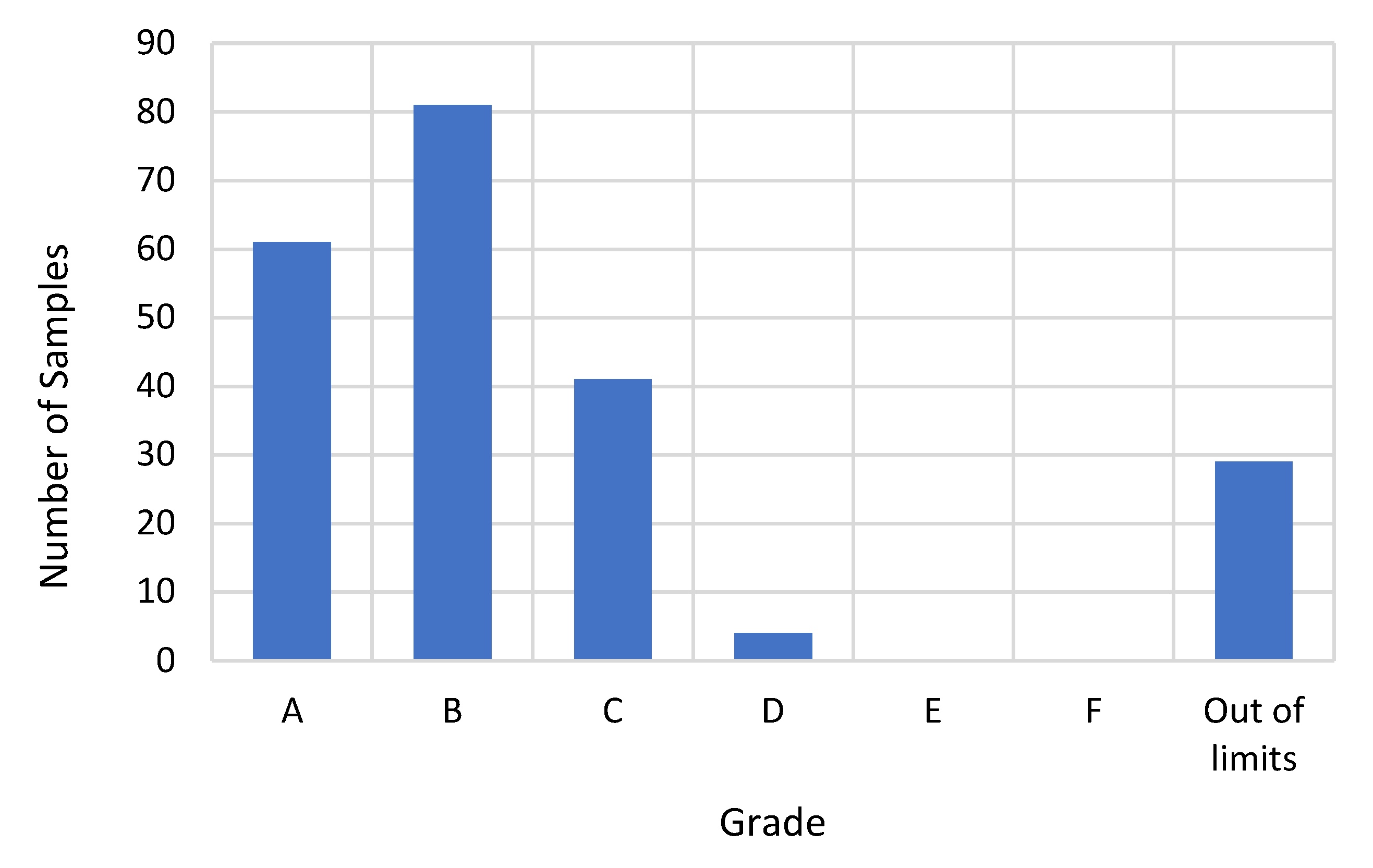
2.1. Aggregate Base Types Selection

A total of 64 aggregate base samples were collected from multiple construction sites across Egypt in order to be tested and used in the development of the prediction models. According to the Egyptian code for urban and rural roads (ECP, 2008) part (4) [29], there are multiple aggregate types or grades used for the base course as shown in

Table 1. Aggregate base gradations used in Egypt [29].

Sieve Size	Limits
	A		B		C		D		E		F
	Min	Max	Min	Max	Min	Max	Min	Max	Min	Max	Min	Max
% Passing from sieve 2 in	100	100	100	100	100	100
% Passing from sieve 1.5 in			70	100			100	100
% Passing from sieve 1 in			55	85	75	95	70	100	100	100	100	100
% Passing from sieve 3/4 in			50	80			60	90			70	100
% Passing from sieve 3/8 in	30	65	40	70	40	75	45	75	50	85	50	80
% Passing from sieve number 4	25	55	30	60	30	60	30	60	35	65	35	65
% Passing from sieve number 10	15	40	20	50	20	45	20	50	25	50	25	50
% Passing from sieve number 40	8	20	10	30	15	30	10	30	15	30	15	30
% Passing from sieve number 200	2	8	5	15	5	20	5	15	5	15	5	15

.

Between 2015 and 2016, almost 216 aggregate base samples were collected and tested from different locations all over Egypt under the supervision of the highway and research laboratory, Cairo University, Egypt. Out of these 216 samples, 61 samples follow grade A, 81 follow grade B, 41 follow grade C, and 4 follow grade D. Figure 2 shows the number of samples that follow the different gradations. Thus, the dataset used in this study contains samples that follow these four grades (A, B, C, and D) with approximately the same percentage of each gradation. The basic tests needed for this study were conducted according to the British Standard practice (BS 1377) [30]. These tests are the specific gravity, aggregate sieve size, Atterberg limits, and the standard Proctor test, during which a standard energy of 592 kJ/m³ should be applied.

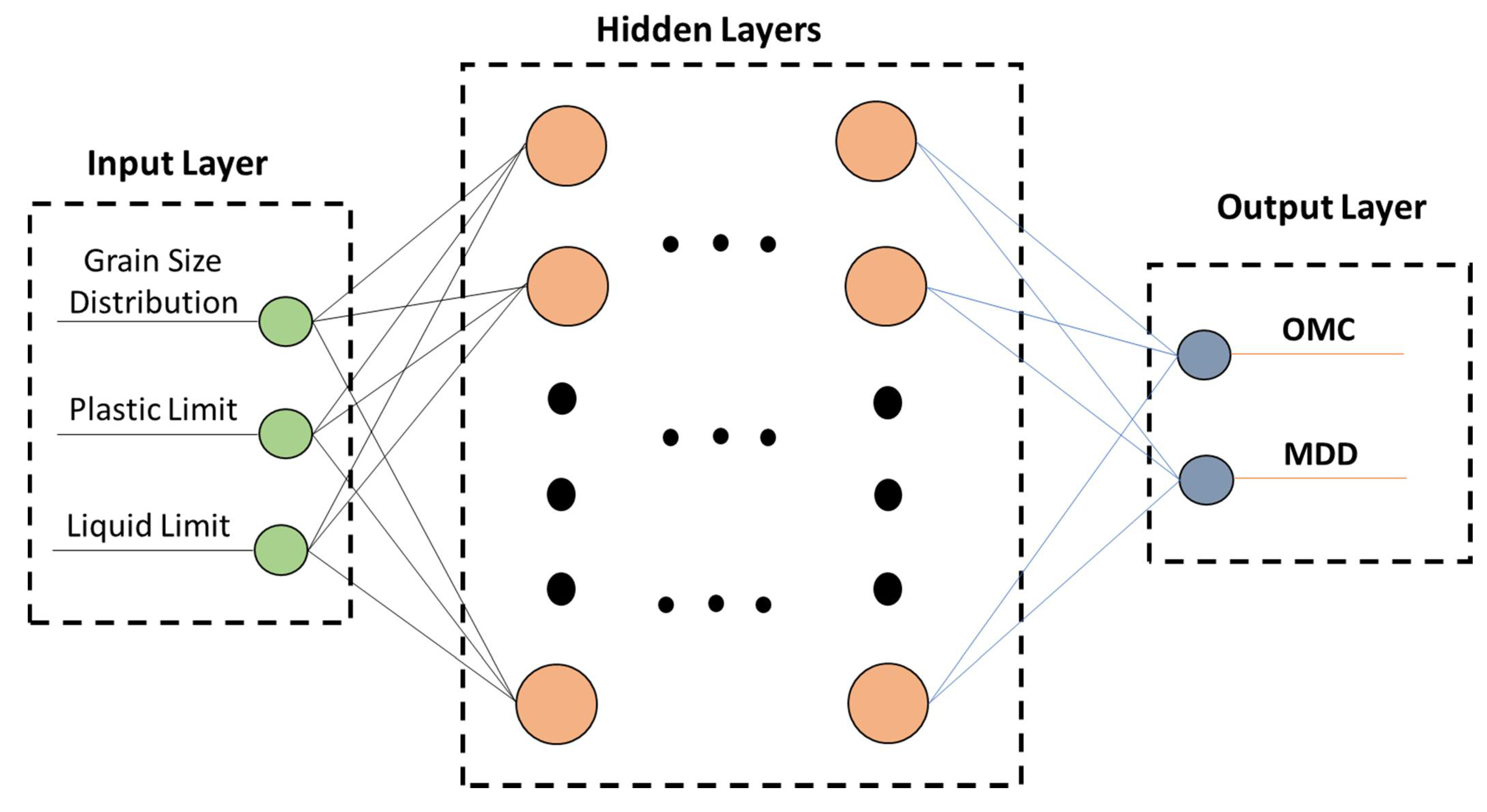
2.2. Artificial Neural Networks

Over the past few years, artificial neural networks have been used as a powerful tool for the prediction problem. Thus, this technique has been employed for the prediction problem in the civil engineering field, and in the pavement engineering field. For example, Othman and Abdelwahab (2021) [3] utilized ANNs for predicting the optimum asphalt content of hot mix asphalt samples. Similarly, Othman [31] utilized ANNs to develop prediction models that can be used for predicting the characteristics of the hot asphalt mixes. Additionally, ANNs have been used in a number of studies for the prediction of the soil properties such as the study by Ardakani and Kordnaeij (2017) [25], the study by Sinha and Wang (2006) [16], the study by Özbeyaz, and Soylemez (2020) [28], and the study by Othman and Abdelwhab [32]. In general, ANN is a system that tries to mimic the human brain system or the neural system. The basic architecture of an ANN consists of three layers and each layer has its own function, starting with the input layer that is responsible for receiving the input information. Next is the hidden layer, which is responsible for receiving signals from the input layer and manipulating this information. Finally, the output layer is responsible for generating the output values or signals [33]. The main unit of the ANN is the neuron, and the neuron is responsible for receiving the input values and modulate its response using an activation function. This activation function is responsible for transmitting the outgoing signals. Each neuron computes a weighted sum of elements of the input vector (Xs) through weights associated with the connections (W) [34] and used the activation function to generate the outputs on the weighted sum of the input values as follows:

$$RH=WX+B$$

(2)

$$Y=F\left(H\right)$$

(3)

In general, there are multiple types of ANNs such as the feedforward and feedback ANNs. Additionally, there are a variety of methods for the training of any ANN such as the supervised and unsupervised learning algorithms. In this study, the supervised backpropagation technique will be used for solving the prediction problem or for the training of the ANN. The main objective of the training process, which is iterative, is to adjust the connection weights in a way that improves the performance of the ANN in the prediction process. The performance of the ANN is significantly influenced by the hyperparameters and the architecture of the ANN. As a result, in this study, multiple ANNs with different hyperparameters are tested in order to choose the optimum ANN configuration and settings that provide the best predictions. The main focus of this paper will be on the effect on the number of hidden layers, number of neurons per hidden layer, and the activation function on the ANNs prediction performance.

In general, the activation function might take multiple expressions. In this study, the main focus will be on three activation functions as follows:

-

The Linear activation function, also called the Rectified Linear Unit (ReLU) function

$$f\left(x\right)=\{\begin{array}{c}xx>0\\ 0x<0\end{array}$$

(4)

-

The logistic activation function, also called the sigmoid function

$$f\left(x\right)=\frac{1}{1+e^{-x}}$$

(5)

-

The hyperbolic activation function, also called the tanh activation function

$$f\left(x\right)=\frac{e^x-e^{-x}}{e^x+e^{-x}}$$

(6)

For every activation function, multiple ANN architectures are tested with different numbers of hidden layers and of neurons per layer. For every activation function, 80 different ANN architectures are tested, starting from an ANN with one hidden layer to an ANN with 4 hidden layers. Moreover, for every hidden layer, different numbers of neurons per layer are tested, starting from 1 neuron per layer to 20 neurons per layer. Figure 3 shows the proposed general ANN structure followed in this paper. The number of hidden layer and neurons per hidden layers used in this study are based on the architectures of ANNs that were tested in previous studies as the maximum number of layers tested in the previous studies is four, and the maximum number of neurons employed in previous studies is 20 neurons per hidden layer [3,16,25,28,31]. Additionally, the weights of the connections are randomly assigned before launching the training process. Then, the ANNs are trained for one thousand iterations. The dataset used in this study was divided into three sets: training set with 40 samples or 62.5%, validation set with 12 samples or 18.75%, and testing set with 12 samples or 18.75%. The training dataset is used for the ANN learning (or training) process, by adjusting the weight and bias vectors to minimize the differences between the outputs and the targets. The validation dataset is used to monitor the convergence of the ANN learning process, and it is often used to avoid overfitting so that the ANN model is applicable to new inputs beyond the ones used in training or validating the ANN model. The testing dataset is used to check the performance of the trained ANN once completed. As shown in the introduction, the effect of index properties and grain size distribution on compacted soils. In addition, the tests to determine the index properties have fairly easy and inexpensive procedures compared with the compaction tests. Thus, in this study, Julia programming language is utilized in order to construct the different ANNs using the PL, LL, and grain size distribution as the inputs to the ANNs. Additionally, the ANNs were to minimize the mean square error using the gradient descent optimization algorithm.

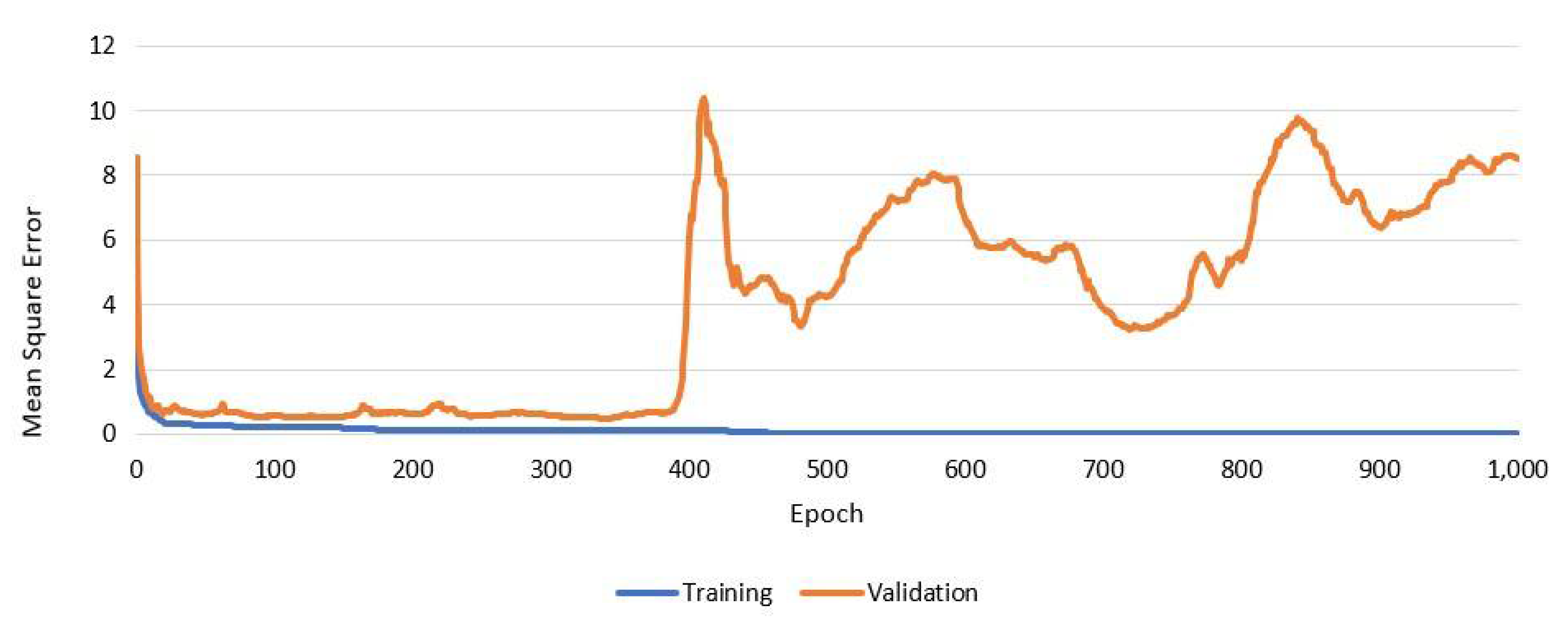
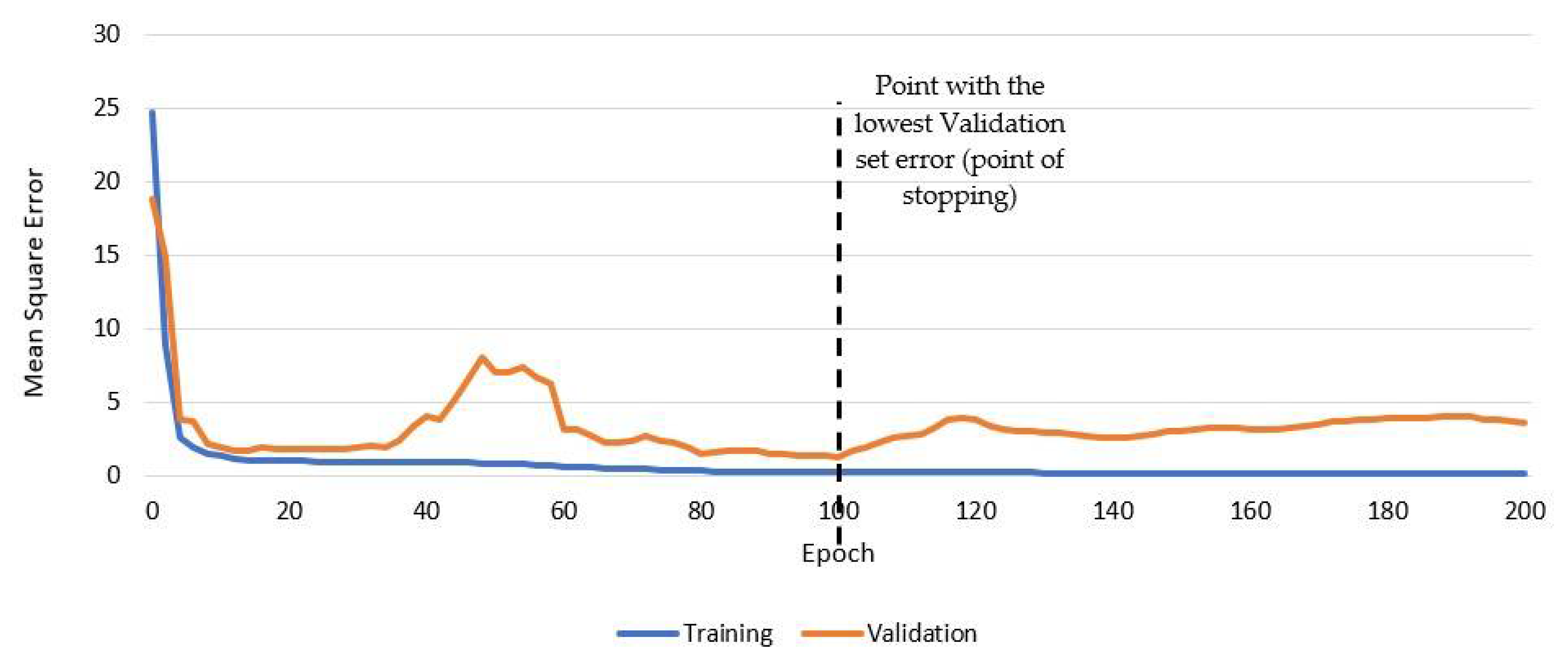
2.3. Early Stopping to Avoid Overfitting

Overfitting during the training process results in deteriorating the ability of the ANN in generalization and in turn results in untrustworthy performance when the ANN is tested in a new dataset. Thus, the main objective of the methods that avoids overfitting is to find the optimum solution in the parameter space according to a predefined criterion. The most common method followed in the literature to avoid overfitting is the early stopping technique [35,36,37,38]. In this technique, the validation set is used to define the stopping criteria at which the training process should be halted. In the simplest condition, the training process should be halted when the validation set error increases during the process of training (while the training set error keeps decreasing). However, the stochastic nature of the training process of the training process might result in a decrease in the validation set error at any point. In other words, the first overfitting point is not always the best point to halt the training process. Consequently, it is recommended to keep the training process for a number of iterations even with the occurrence of overfitting, and to keep monitoring the validation set error. If the error of the validation set keeps increasing, the training process should be halted. On the other hand, if the error of the validation set declines again, the training process should continue [39]. In this study, the early stopping technique was used to avoid overfitting. Additionally, 100 iterations are used to monitor the validation set error. After these 100 iterations, if the validation set error declined again the training process proceeds, otherwise the training process is halted. Figure 4 shows one example for the validation set and training set errors during 1000 iterations of the training process. The figure shows how the validation set error fluctuates during the training process and how the overtraining of the ANN leads to overfitting as the validation set error increases significantly while the training set error keeps declining. Additionally, the application of the early stopping techniques for one example is shown in Figure 5, and the figure shows how the validation set error fluctuates up and down within a small number of iterations; in this case, the training process is halted when the validation set error increased and did not decrease again for 100 iterations.

2.4. ANN Performance Evaluation

The selection of the optimum ANN hyperparameters should be based on the evaluation of the ability or accuracy of every ANN to predict the output value, which is achieved through statistical indicators. The most common statistical indicator is the coefficient of determination (R²) and it has a value ranged from 0 to 1, where a value of 1 indicates that the model perfectly fits the data and the closest the value to 1, the better the predictions of the model. The coefficient of determination is calculated as follows:

$$R^2=\frac{{{\displaystyle \sum }}_n{\left(h_i-t_i\right)}^2}{{{\displaystyle \sum }}_n{\left(h_i-\overline{\left(h_i\right)}\right)}^2}$$

(7)

where, h_i. = the prediction of the ANN, $t_i$ = the true value, and $\overline{h_i}$ = the average of the predictions of the ANN.

3. Results and Analysis

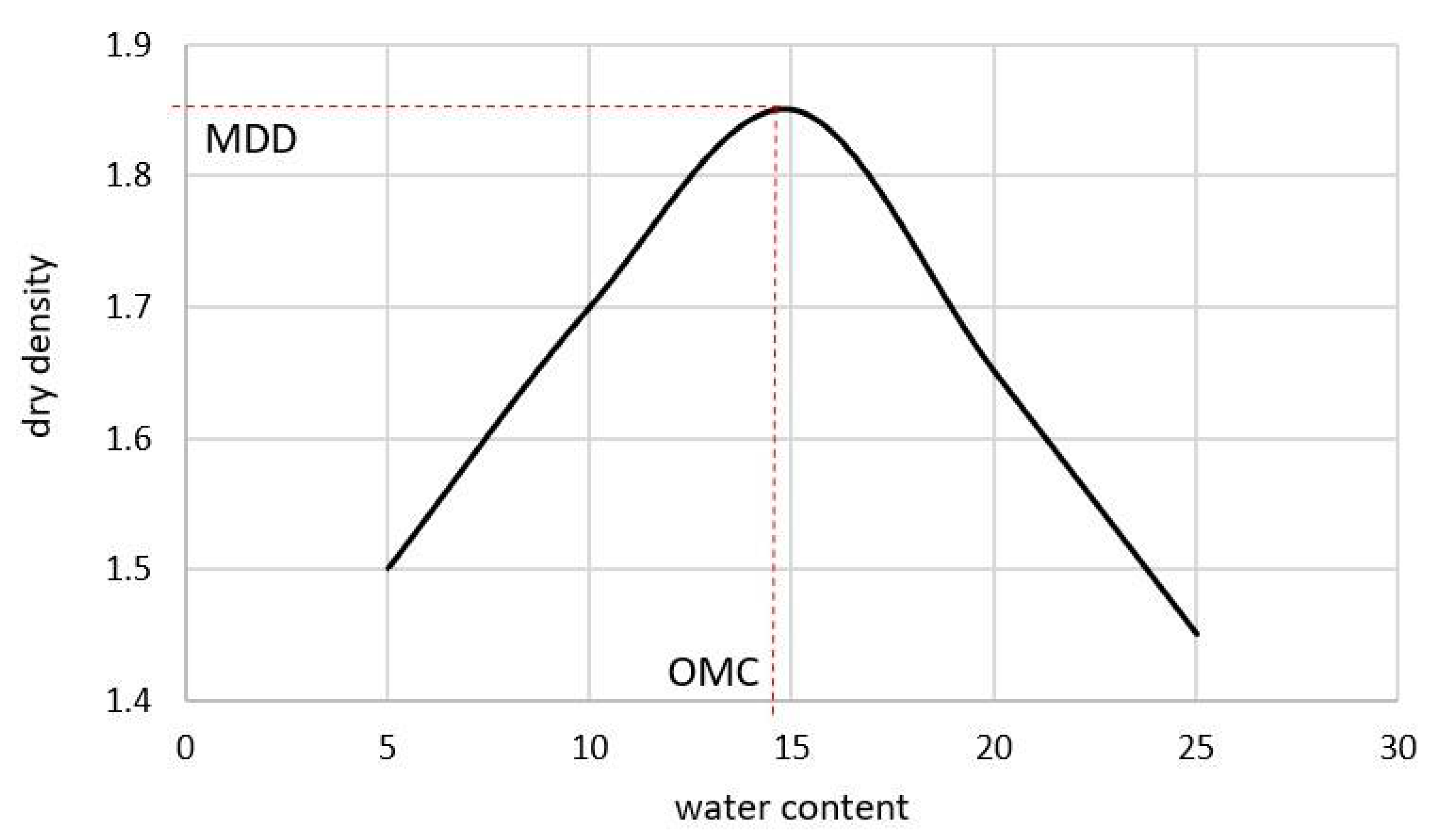
The coefficient of determination for every ANN when used on the testing set is shown in

Table 2. R² values of the testing set for every ANN in the prediction of the MDD.

MDD		Number of Hidden Layers
		ReLu Activation Function				Sigmoid Activation Function				Tanh Activation Function
		1	2	3	4	1	2	3	4	1	2	3	4
Number of Nuerons per Hidden Layer	1	0.807	0.768	0.789	0.773	0.89	0.894	0.727	0.777	0.903	0.659	0.614	0.892
	2	0.698	0.798	0.771	0.806	0.832	0.867	0.796	0.779	0.877	0.675	0.715	0.648
	3	0.75	0.759	0.752	0.729	0.843	0.809	0.687	0.744	0.708	0.792	0.559	0.844
	4	0.814	0.718	0.737	0.711	0.863	0.876	0.714	0.793	0.665	0.668	0.748	0.48
	5	0.677	0.777	0.816	0.793	0.79	0.649	0.829	0.747	0.652	0.882	0.471	0.754
	6	0.696	0.817	0.772	0.758	0.75	0.608	0.752	0.548	0.585	0.784	0.756	0.683
	7	0.66	0.656	0.777	0.8	0.768	0.741	0.756	0.761	0.778	0.709	0.781	0.42
	8	0.766	0.791	0.775	0.757	0.785	0.835	0.711	0.743	0.636	0.772	0.868	0.478
	9	0.831	0.761	0.697	0.683	0.863	0.86	0.805	0.675	0.473	0.544	0.294	0.773
	10	0.644	0.71	0.73	0.652	0.739	0.852	0.877	0.648	0.841	0.779	0.489	0.498
	11	0.651	0.715	0.742	0.675	0.811	0.684	0.843	0.725	0.621	0.599	0.455	0.936
	12	0.728	0.648	0.657	0.63	0.724	0.631	0.721	0.76	0.451	0.762	0.664	0.796
	13	0.692	0.653	0.657	0.657	0.707	0.765	0.549	0.604	0.538	0.756	0.797	0.392
	14	0.773	0.718	0.64	0.653	0.632	0.498	0.739	0.644	0.667	0.624	0.885	0.493
	15	0.73	0.663	0.649	0.644	0.748	0.529	0.81	0.69	0.51	0.656	0.711	0.349
	16	0.754	0.658	0.653	0.657	0.765	0.827	0.532	0.651	0.447	0.904	0.52	0.228
	17	0.656	0.653	0.727	0.75	0.799	0.768	0.742	0.651	0.587	0.574	0.749	0.292
	18	0.642	0.655	0.553	0.685	0.621	0.411	0.572	0.669	0.497	0.766	0.315	0.596
	19	0.656	0.614	0.675	0.657	0.654	0.746	0.752	0.563	0.694	0.491	0.782	0.231
	20	0.644	0.635	0.638	0.649	0.894	0.629	0.579	0.668	0.532	0.712	0.687	0.318

and

Table 3. R² values of the testing set for every ANN in the prediction of the OMC.

OMC		Number of Hidden Layers
		ReLu Activation Function				Sigmoid Activation Function				Tanh Activation Function
		1	2	3	4	1	2	3	4	1	2	3	4
Number of Neurons per Hidden Layer	1	0.79	0.766	0.781	0.783	0.848	0.92	0.814	0.832	0.928	0.821	0.772	0.93
	2	0.724	0.812	0.75	0.8	0.878	0.929	0.817	0.836	0.794	0.69	0.575	0.458
	3	0.767	0.803	0.784	0.707	0.826	0.846	0.771	0.802	0.814	0.777	0.655	0.887
	4	0.756	0.668	0.671	0.725	0.798	0.846	0.717	0.785	0.625	0.52	0.818	0.538
	5	0.785	0.867	0.754	0.729	0.874	0.63	0.896	0.687	0.547	0.558	0.486	0.683
	6	0.793	0.754	0.675	0.755	0.75	0.61	0.82	0.527	0.662	0.568	0.83	0.635
	7	0.773	0.717	0.711	0.65	0.638	0.642	0.771	0.774	0.77	0.617	0.452	0.772
	8	0.796	0.794	0.769	0.734	0.731	0.714	0.684	0.752	0.636	0.775	0.273	0.335
	9	0.704	0.644	0.779	0.679	0.862	0.792	0.699	0.627	0.685	0.573	0.744	0.591
	10	0.87	0.579	0.604	0.613	0.683	0.535	0.732	0.724	0.739	0.693	0.364	0.215
	11	0.629	0.672	0.669	0.603	0.558	0.753	0.676	0.571	0.595	0.478	0.37	0.72
	12	0.662	0.596	0.604	0.68	0.726	0.498	0.719	0.728	0.426	0.931	0.291	0.478
	13	0.615	0.6	0.611	0.733	0.705	0.742	0.801	0.66	0.312	0.795	0.469	0.563
	14	0.852	0.679	0.654	0.598	0.683	0.523	0.732	0.801	0.527	0.845	0.636	0.28
	15	0.644	0.698	0.608	0.591	0.566	0.726	0.684	0.703	0.533	0.573	0.783	0.223
	16	0.825	0.634	0.585	0.663	0.79	0.714	0.681	0.625	0.629	0.357	0.263	0.28
	17	0.629	0.622	0.556	0.577	0.843	0.546	0.812	0.428	0.464	0.462	0.59	0.308
	18	0.612	0.617	0.76	0.665	0.696	0.734	0.533	0.621	0.305	0.613	0.23	0.435
	19	0.615	0.599	0.591	0.595	0.606	0.595	0.79	0.403	0.507	0.469	0.424	0.15
	20	0.644	0.633	0.622	0.617	0.76	0.467	0.555	0.719	0.545	0.525	0.608	0.744

. In order to easily visualize the values, the cells are highlighted from red which indicates the lowest R² value to green which indicates the highest R² value.

3.1. MDD

Table 2 shows the predicting capability (performance) of every ANN in estimating the MDD. The table illustrates that the ReLu activation function provides the lowest level of accuracy when compared with the other two activation functions. Additionally, there is a general pattern that can be observed across the three activation functions. In general, the prediction capability of the ANNs deteriorates with the increase in the number of hidden layers per neurons and with the number of neurons per hidden layer. In general, the simpler the ANN, the better the performance. However, the ANN that offers the best MDD predictions utilizes the tanh activation function and consists of 4 hidden layers and 11 neurons per hidden layers. This ANN has the ability to predict the MDD with an R² value of 0.936. On the other hand, this optimum ANN performs moderately in the prediction of the OMC as it has an R² value of 0.72 as shown in Table 3.

3.2. OMC

Table 3 shows the predicting capability (performance) of every ANN in estimating the MDD. The table illustrates that the ReLu activation function provides the lowest level of accuracy when compared with the other two activation functions. Additionally, there is a general pattern that can be observed across the three activation functions. In general, the prediction capability of the ANNs deteriorates with the increase in the number of hidden layers per neurons and with the number of neurons per hidden layer. In general, the simpler the ANN, the better the performance. On the other hand, the ANN that offers the best OMC predictions utilizes the tanh activation function and consists of 2 hidden layers and 12 neurons per hidden layers. This ANN has the ability to predict the OMC with an R² value of 0.931. On the other hand, this optimum ANN performs moderately in the prediction of the MDD as it has an R² value of 0.762 as shown in Table 2.

3.3. Optimum ANN Architecture for the Predictions of Both the OMC and MDD

The previous two subsections focus on finding the optimum ANN for predicting one of the two compaction parameters. However, the two ANNs can predict one variable with high level of accuracy and perform moderately for the other variable. However, the main objective of this study is to find the optimum ANN that has the ability to estimate the two compaction parameters with low error, especially as we are training the ANN for estimating the two variables. Thus, the main objective of this subsection is to search for the optimum ANN that is able to estimate the two compaction parameters with high level of accuracy, instead of finding the ANN the optimizes the performance for only one output. As a result, a new R² value is calculated for every ANN as follows:

$$R_{new}^2=\frac{R_{OMC}^2}{2}+\frac{R_{MDD}^2}{2}$$

(8)

The updated R² values are shown in

Table 4. R² values of the testing set for every ANN in the prediction of both the OMC and MDD.

Balanced		Number of Hidden Layers
		ReLu Activation Function				Sigmoid Activation Function				Tanh Activation Function
		1	2	3	4	1	2	3	4	1	2	3	4
Number of Neurons per Hidden Layer	1	0.7985	0.767	0.785	0.778	0.869	0.907	0.7705	0.8045	0.9155	0.74	0.693	0.911
	2	0.711	0.805	0.7605	0.803	0.855	0.898	0.8065	0.8075	0.8355	0.6825	0.645	0.553
	3	0.7585	0.781	0.768	0.718	0.83s45	0.8275	0.729	0.773	0.761	0.7845	0.607	0.8655
	4	0.785	0.693	0.704	0.718	0.8305	0.861	0.7155	0.789	0.645	0.594	0.783	0.509
	5	0.731	0.822	0.785	0.761	0.832	0.6395	0.8625	0.717	0.5995	0.72	0.4785	0.7185
	6	0.7445	0.7855	0.7235	0.7565	0.75	0.609	0.786	0.5375	0.6235	0.676	0.793	0.659
	7	0.7165	0.6865	0.744	0.725	0.703	0.6915	0.7635	0.7675	0.774	0.663	0.6165	0.596
	8	0.781	0.7925	0.772	0.7455	0.758	0.7745	0.6975	0.7475	0.636	0.7735	0.5705	0.4065
	9	0.7675	0.7025	0.738	0.681	0.8625	0.826	0.752	0.651	0.579	0.5585	0.519	0.682
	10	0.757	0.6445	0.667	0.6325	0.711	0.6935	0.8045	0.686	0.79	0.736	0.4265	0.3565
	11	0.64	0.6935	0.7055	0.639	0.6845	0.7185	0.7595	0.648	0.608	0.5385	0.4125	0.828
	12	0.695	0.622	0.6305	0.655	0.725	0.5645	0.72	0.744	0.4385	0.8465	0.4775	0.637
	13	0.6535	0.6265	0.634	0.695	0.706	0.7535	0.675	0.632	0.425	0.7755	0.633	0.4775
	14	0.8125	0.6985	0.647	0.6255	0.6575	0.5105	0.7355	0.7225	0.597	0.7345	0.7605	0.3865
	15	0.687	0.6805	0.6285	0.6175	0.657	0.6275	0.747	0.6965	0.5215	0.6145	0.747	0.286
	16	0.7895	0.646	0.619	0.66	0.7775	0.7705	0.6065	0.638	0.538	0.6305	0.3915	0.254
	17	0.6425	0.6375	0.6415	0.6635	0.821	0.657	0.777	0.5395	0.5255	0.518	0.6695	0.3
	18	0.627	0.636	0.6565	0.675	0.6585	0.5725	0.5525	0.645	0.401	0.6895	0.2725	0.5155
	19	0.6355	0.6065	0.633	0.626	0.63	0.6705	0.771	0.483	0.6005	0.48	0.603	0.1905
	20	0.644	0.634	0.63	0.633	0.827	0.548	0.567	0.6935	0.5385	0.6185	0.6475	0.531

and the results show that the ReLu activation function provides the lowest level of accuracy when compared with the other two activation functions (ReLu and sigmoid). Additionally, the performance of the ANNs deteriorate with the increase in the number of hidden layers per neurons and with the number of neurons per hidden layer. Moreover, the optimum ANN that predicts the OMC and MDD utilizes the tanh activation function and consists of one hidden layer, and one neuron in this hidden layer. This ANN can predict the MDD with an R² value of (0.903) and can predict the OMC with an R² value of (0.928). Additionally, there are multiple ANNs that can achieve similar results. These ANNs are simple and consist of one or two neurons per hidden layers and employ either the logistic or the tanh activation function. A comparison between the prediction of the ANN that produces the best OMC, the ANN that produces the best MDD, and the ANN that produces the best predictions for both outputs is shown in

Table 5. Comparison between the optimum ANN for every output and the optimum ANN for the two outputs.

	Optimum ANN for Every Output					Optimum ANN for Both Predictions				R2 Difference
	Hidden Layers	Neurons/Layer	Activation Function	R2 (MDD)	R2 (OMC)	Hidden Layers	Neurons/Layer	Activation Function	R2
MDD	4	11	Tanh	0.936	0.72	1	1	Tanh	0.903	0.033
OMC	2	12	Tanh	0.762	0.931				0.928	0.003

. Results show that the difference in the R² values between the optimum ANN for both predictions and the optimum ANN for every prediction individually are 3.3% for the MDD and 0.3% for the OMC and those differences are minor.

3.4. Comparing Previous Studies with the Proposed ANN

This subsection focuses on validating the proposed optimum ANN and compares its performance with the previously proposed ANNs in the literature. This comparison focuses on comparing the performance of these ANNs on the testing set database as reported in every study.

Table 6. The performance of the ANNs proposed in the literature and the proposed ANN in this study.

Study	R2 for the OMC	R2 for the MDD
Günaydın (2009) [22]	0.837	0.793
Alavi et al. (2010) [40]	0.89	0.91
Kurnaz and Kaya (2020) [41]	0.85	0.86
Özbeyaz and Solyemez (2020) [28]	0.83	0.71
Proposed ANN	0.903	0.928

summarizes the performance of every ANN and the final raw shows the coefficient of determination of the optimum ANN proposed in this study. Comparing the R² values in the table shows that the ANN proposed in the current study outperforms the ANNs proposed in the literature, as the previous studies did not carry out a comprehensive search to reach the optimum ANN, but considered limited ANNs with specific assumptions. On the other hand, in this study, a comprehensive search was conducted to choose the optimum activation function and the optimum architecture that achieve the best performance.

4. Multiple Linear Regression (MLR)

In order to the validate results of the ANN, multiple linear regression models were developed and compared with the results of the ANN. During the model development process, the backward elimination technique was used to exclude the insignificant variables. In the backward elimination, all independent variables are entered in the model and each one is deleted one at a time if they do not contribute to the regression equation. The inputs used for developing the MLR models are the same as the inputs used for developing the ANN models. These inputs are the sieve analysis and Atterberg limits.

Table 7. Details of the MLR models developed for the MDD during the backward elimination process.

Model	Excluded Variables	R	R Square	Adjusted R Square	Std. Error of the Estimate
1	-	0.646	0.418	0.281	0.070509
2	%P (1.5 in)	0.646	0.418	0.295	0.069828
3	%P (1.5 in), %P (3/8 in)	0.646	0.417	0.307	0.069194
4	%P (1.5 in), %P (3/8 in), %P(2 in)	0.646	0.417	0.32	0.068589
5	%P (1.5 in), %P (3/8 in), %P(2 in), LL	0.643	0.414	0.329	0.068118
6	%P (1.5 in), %P (3/8 in), %P(2 in), LL, %P(0.5 in)	0.635	0.403	0.329	0.068119
7	%P (1.5 in), %P (3/8 in), %P(2 in), LL, %P(0.5 in), %P (3/4 in)	0.630	0.396	0.333	0.067909
8	%P (1.5 in), %P (3/8 in), %P(2 in), LL, %P(0.5 in), %P (1 in)	0.628	0.395	0.343	0.067409

Where: %P(i) = Percentage of the passing from sieve (i).

and

Table 8. Details of the MLR models developed for the OMC during the backward elimination process.

Model	Excluded Variables	R	R Square	Adjusted R Square	Std. Error of the Estimate
1	-	0.673	0.453	0.325	1.4857
2	%P (#4)	0.673	0.453	0.338	1.4714
3	%P (#4), %P(0.5 in)	0.673	0.452	0.349	1.4586
4	%P (#4), %P(0.5 in), %P(2 in)	0.672	0.451	0.36	1.4467
5	%P (#4), %P(0.5 in), %P(2 in), %P (1.5 in)	0.671	0.45	0.37	1.4349
6	%P (#4), %P(0.5 in), %P(2 in), %P (1.5 in), LL	0.670	0.448	0.379	1.4244
7	%P (#4), %P(0.5 in), %P(2 in), %P (1.5 in), LL, %P (3/8 in)	0.658	0.433	0.373	1.4313
8	%P (#4), %P(0.5 in), %P(2 in), %P (1.5 in), LL, %P (3/8 in), %P (#10)	0.650	0.423	0.373	1.4312
9	%P (#4), %P(0.5 in), %P(2 in), %P (1.5 in), LL, %P (3/8 in), %P (#10), %P(#40)	0.644	0.415	0.375	1.4288
10	%P (#4), %P(0.5 in), %P(2 in), %P (1.5 in), LL, %P (3/8 in), %P (#10), %P(#40), %P (3/4 in)	0.638	0.407	0.377	1.4271
11	%P (#4), %P(0.5 in), %P(2 in), %P (1.5 in), LL, %P (3/8 in), %P (#10), %P(#40), %P (3/4 in), %P (1in)	0.627	0.393	0.374	1.4311

Where: %P(i) = Percentage of the passing from sieve (i).

summarize the details of the models developed during the backward elimination process for both the MDD and OMD.

Table 9. MDD prediction model.

Model-8	Unstandardized Coefficients		Standardized Coefficients	t	Sig.
	B	Std. Error	Beta
(Constant)	2.289	0.069		32.942	0
Passing Sieve Number 4	0.009	0.004	0.649	2.176	0.034
Passing Sieve Number 10	−0.015	0.007	−0.984	−2.114	0.039
Passing Sieve Number 40	0.01	0.006	0.664	1.852	0.045
PassingSieveNO200	−0.015	0.003	−0.771	−4.252	0
Plastic Limit	−0.005	0.003	−0.191	−1.815	0.048

and

Table 10. OMC prediction model.

Model-11	Unstandardized Coefficients		Standardized Coefficients	t	Sig.
	B	Std. Error	Beta
(Constant)	2.957	1.092		2.708	0.009
Passing Sieve number 200	0.239	0.041	0.577	5.763	0
PlasticLimit	0.105	0.053	0.198	1.974	0.05

show the details of the final models developed at the end of the backward elimination process for both the OMC and MDD.

The previous tables show that the MLR technique has low R² values of 0.395 and 0.393 for the prediction of the MDD and OMC. Thus, comparing the coefficient of determination of the ANN and MLR techniques shows that the ANN outperforms the traditional regression analysis technique.

Table 11. R² values of the different ANNs proposed and the MLR technique.

R-Square Value
MLR		Optimum ANN for the MDD		Optimum ANN for the OMC		Optimum ANN for Both OMC and MDD
MDD	OMC	MDD	OMC	MDD	OMC	MDD	OMC
0.395	0.393	0.936	0.72	0.931	0.762	0.903	0.928

summarizes the comparison between the ANN and the MLR techniques in predicting the OMC and MDD.

5. Conclusions

The present study focuses on developing ANNs models for estimating the compaction parameters of the aggregate base course used in constructing roads in Egypt using the aggregate gradation and Atterberg limits as the inputs to the ANNs. A total of 240 different ANNs were tested with different structures and hyperparameters in order to select the ANN that offered the lowest error based on the results of 64 aggregate base samples that were tested on the standard Proctor test. The results of this study can be summarized as follows:

-

The optimum structure and hyperparameters of the ANN changes depending on the desired output, as shown in

Table 12. The optimum ANN for every output.

	Optimum ANN for Every Output
	Hidden Layers	Neurons/Layer	Activation Function
MDD	4	11	Tanh
OMC	2	12	Tanh
Both (OMC and MDD)	1	1	Tanh

.

-

In general, the tanh activation function is the most efficient, as it outperforms the other two activation functions. Additionally, the simpler the ANN architecture, the better the predictions, as the performance of the ANNs deteriorates with the increase in the number of hidden layers or the number of neurons per hidden layers.

-

The optimum ANN proposed can be used for estimating the OMC and MDD of the aggregate base course in Egypt with high accuracy (R² = 0.903 for OMC, and R² = 0.928 for MDD). Thus, this ANN can be used as an alternative to the standard Proctor test and, in this case, it can save significant time, material, and effort.

-

The results show that the proposed ANN outperforms the MLR models and offers highly accurate predictions.

While this study focuses on the estimation of the OMC and MDD of the aggregate base course, it is highly recommended to replicate the analysis for the subgrade course. Additionally, while the specifications for the aggregate base course vary from country to country, it is highly recommended to replicate the same analysis for aggregate base samples collected from other countries; the present analysis can be used as a benchmark for the new analysis.

References

1. Rakaraddi, P.G.; Gomarsi, V. Establishing Relationship between CBR with Different Soil Properties. Int. J. Res. Eng. Technol. 2015, 4, 182–188. [Google Scholar]
2. Mousa, K.M.; Abdelwahab, H.T.; Hozayen, H.A. Models for estimating optimum asphalt content from aggregate gradation. Proc. Inst. Civ. Eng.-Constr. Mater. 2018, 174, 69–74. [Google Scholar] [CrossRef]
3. Othman, K.M.M.; Abdelwahab, H. Prediction of the optimum asphalt content using artificial neural networks. Met. Mater. Eng. 2021, 27. [Google Scholar] [CrossRef]
4. HMA Pavement Mix Type Selection Guide; Information Serise, 128; National Asphalt Pavement Association: Lanham, MD, USA; Federal Highway Administration: Washington, DC, USA, 2001.
5. Sridharan, A.; Nagaraj, H.B. Plastic limit and compaction characteristics of finegrained soils. Proc. Inst. Civ. Eng.-Ground Improv. 2005, 9, 17–22. [Google Scholar] [CrossRef]
6. Proctor, R. Fundamental Principles of Soil Compaction. Eng. News-Rec. 1933, 111, 245–248. [Google Scholar]
7. Viji, V.K.; Lissy, K.F.; Sobha, C.; Benny, M.A. Predictions on compaction characteristics of fly ashes using regression analysis and artificial neural network analysis. Int. J. Geotech. Eng. 2013, 7, 282–291. [Google Scholar] [CrossRef]
8. ASTM International. D 698: Standard Test Methods for Laboratory Compaction Characteristics Of Soil Using Standard Effort (12 400 Ftlbf/ft3 (600 Kn-m/m3); ASTM International: West Conshohocken, PA, USA, 2012. [Google Scholar]
9. Zainal, A.K.E. Quick Estimation of Maximum Dry Unit Weight and Optimum Moisture Content from Compaction Curve Using Peak Functions. Appl. Res. J. 2016, 2, 472–480. [Google Scholar]
10. Jumikis, A.R. Geology of Soils of the Newark (NJ) Metropolitan Area. J. Soil Mech. Found. ASCE 1946, 93, 71–95. [Google Scholar]
11. Jumikis, A.R. Geology of Soils of the Newark (NJ) Metropolitan Area. J. Soil Mech. Found. Div. 1958, 84, 1–41. [Google Scholar] [CrossRef]
12. Ring, G.W.; Sallberg, J.R.; Collins, W.H. Correlation Of Compaction and Classification Test Data. Highw. Res. Board Bull. 1962, 325, 55–75. [Google Scholar]
13. Ramiah, B.K.; Viswanath, V.; Krishnamurthy, H.V. Interrelationship of compaction and index properties. In Proceedings of the 2nd South East Asian Conference on Soil Engineering, Singapore, 11–15 June 1970; Volume 587. [Google Scholar]
14. Hammond, A.A. Evolution of One Point Method for Determining The Laboratory Maximum Dry Density. Proc. ICC 1980, 1, 47–50. [Google Scholar]
15. Wang, M.C.; Huang, C.C. Soil Compaction and Permeability Prediction Models. J. Environ. Eng. 1984, 110, 1063–1083. [Google Scholar] [CrossRef]
16. Sinha, S.K.; Wang, M.C. Artificial Neural Network Prediction Models for Soil Compaction and Permeability. Geotech. Geol. Eng. 2007, 26, 47–64. [Google Scholar] [CrossRef]
17. Al-Khafaji, A.N. Estimation of soil compaction parameters by means of Atterberg limits. Q. J. Eng. Geol. Hydrogeol. 1993, 26, 359–368. [Google Scholar] [CrossRef]
18. Blotz, L.R.; Benson, C.H.; Boutwell, G.P. Estimating Optimum Water Content and Maximum Dry Unit Weight for Compacted Clays. J. Geotech. Geoenviron. Eng. 1998, 124, 907–912. [Google Scholar] [CrossRef]
19. Gurtug, Y.; Sridharan, A. Compaction Behaviour and Prediction of its Characteristics of Fine Grained Soils with Particular Reference to Compaction Energy. Soils Found. 2004, 44, 27–36. [Google Scholar] [CrossRef] [Green Version]
20. Suits, L.D.; Sheahan, T.; Sridharan, A.; Sivapullaiah, P. Mini Compaction Test Apparatus for Fine Grained Soils. Geotech. Test. J. 2005, 28, 240–246. [Google Scholar] [CrossRef]
21. Di Matteo, L.; Bigotti, F.; Ricco, R. Best-Fit Models to Estimate Modified Proctor Properties of Compacted Soil. J. Geotech. Geoenviron. Eng. 2009, 135, 992–996. [Google Scholar] [CrossRef]
22. Günaydın, O. Estimation of soil compaction parameters by using statistical analyses and artificial neural networks. Environ. Earth Sci. 2008, 57, 203–215. [Google Scholar] [CrossRef]
23. Bera, A.; Ghosh, A. Regression model for prediction of optimum moisture content and maximum dry unit weight of fine grained soil. Int. J. Geotech. Eng. 2011, 5, 297–305. [Google Scholar] [CrossRef]
24. Farooq, K.; Khalid, U.; Mujtaba, H. Prediction of Compaction Characteristics of Fine-Grained Soils Using Consistency Limits. Arab. J. Sci. Eng. 2015, 41, 1319–1328. [Google Scholar] [CrossRef]
25. Ardakani, A.; Kordnaeij, A. Soil compaction parameters prediction using GMDH-type neural network and genetic algorithm. Eur. J. Environ. Civ. Eng. 2017, 23, 449–462. [Google Scholar] [CrossRef]
26. Gurtug, Y.; Sridharan, A.; Ikizler, S.B. Simplified Method to Predict Compaction Curves and Characteristics of Soils. Iran. J. Sci. Technol. Trans. Civ. Eng. 2018, 42, 207–216. [Google Scholar] [CrossRef]
27. Hussain, A.; Atalar, C. Estimation of compaction characteristics of soils using Atterberg limits. IOP Conf. Series Mater. Sci. Eng. 2020, 800, 012024. [Google Scholar] [CrossRef]
28. Özbeyaz, A.; Söylemez, M. Modeling compaction parameters using support vector and decision tree regression algorithms. Turk. J. Electr. Eng. Comput. Sci. 2020, 28, 3079–3093. [Google Scholar] [CrossRef]
29. ECP (Egyptian Code Provisions). ECP(104/4): Egyptian Code for Urban and Rural Roads; Part (4): Road Material and Its Tests; Housing and Building National Research Center: Cairo, Egypt, 2008. [Google Scholar]
30. British Standard Institution. BS1377 Methods of Test for Soils for Civil Engineering Purposes; British Standards Institution: London, UK, 1990. [Google Scholar]
31. Othman, K.; Abdelwahab, H. Using Deep Neural Networks for the Prediction of the Optimum Asphalt Content and the Asphalt mix Properties. 2021; in preparation. [Google Scholar]
32. Othman, K.; Abdelwahab, H. Prediction of the Soil Compaction Parameters Using Deep Neural Networks. Transp. Infrastruct. Geotechnol. 2021. [Google Scholar] [CrossRef]
33. Haykin, S. Neural Networks, a Comprehensive Foundation; Prentice Hall: Hoboken, NJ, USA, 1994. [Google Scholar]
34. McCulloch, W.S.; Pitts, W. A logical calculus of the ideas immanent in nervous activity. Bull. Math. Biol. 1943, 5, 115–133. [Google Scholar] [CrossRef]
35. Liu, Y.; Starzyk, J.; Zhu, Z. Optimized Approximation Algorithm in Neural Networks without Overfitting. IEEE Trans. Neural Netw. 2008, 19, 983–995. [Google Scholar] [CrossRef]
36. Piotrowski, A.P.; Napiorkowski, J.J. A comparison of methods to avoid overfitting in neural networks training in the case of catchment runoff modelling. J. Hydrol. 2013, 476, 97–111. [Google Scholar] [CrossRef]
37. Goodfellow, L.; Bengio, Y.; Courville, A. Deep Learning (Adaptive Computation and Machine Learning Series); MIT Press: Cambridge, MA, USA, 2016. [Google Scholar]
38. Christopher, B. Pattern Recognition and Machine Learning (Information Science and Statistics); Springer: Berlin/Heidelberg, Germany, 2006. [Google Scholar]
39. Prechelt, L. Neural Networks: Tricks of the Trade; Lecture Notes in Computer Science; Springer: Berlin/Heidelberg, Germany, 1998; Volume 1524, pp. 53–67. [Google Scholar]
40. Alavi, A.H.; Gandomi, A.H.; Mollahassani, A.; Heshmati, A.A.; Rashed, A. Modeling of maximum dry density and optimum moisture content of stabilized soil using artificial neural networks. J. Plant Nutr. Soil Sci. 2010, 173, 368–379. [Google Scholar] [CrossRef]
41. Kurnaz, T.F.; Kaya, Y. The performance comparison of the soft computing methods on the prediction of soil compaction parameters. Arab. J. Geosci. 2020, 13, 159. [Google Scholar] [CrossRef]
Figure 1. OMC, MDD general curve.
Designs 05 00078 g001
Figure 2. Number of samples for different aggregate gradations.
Designs 05 00078 g002
Figure 3. The general ANN structure followed.
Designs 05 00078 g003
Figure 4. The training set and validation set error during the training process for an ANN with 3 hidden layers, 3 neurons per hidden layer and employs the tanh activation function.
Designs 05 00078 g004
Figure 5. The validation and training sets error during the training process with the application of the early stopping technique for an ANN with 3 hidden layers, 3 neurons per hidden layer and employs the tanh activation function.
Designs 05 00078 g005