Abstract
The development of autonomous vehicles is one of the most active research areas in the automotive industry. The objective of this study is to present a concept for analysing a vehicle’s current situation and a decision-making algorithm which determines an optimal and safe series of manoeuvres to be executed. Our work focuses on a machine learning-based approach by using neural networks for risk estimation, comparing different classification algorithms for traffic density estimation and using probabilistic and decision networks for behaviour planning. A situation analysis is carried out by a traffic density classifier module and a risk estimation algorithm, which predicts risks in a discrete manoeuvre space. For real-time operation, we applied a neural network approach, which approximates the results of the algorithm we used as a ground truth, and a labelling solution for the network’s training data. For the classification of the current traffic density, we used a support vector machine. The situation analysis provides input for the decision making. For this task, we applied probabilistic networks.
1. Introduction
A feasible and appropriate system concept for self-driving cars is receiving more attention as more participants of the automotive industry start developing their own solutions. Situation analysis is one of the key components, as it has to process a large amount of data to provide real-time information about the vehicle’s current situation. This information can be used to plan a series of actions which agree with the objectives of the self-driving function. This is done by behaviour planning algorithms which work at a much higher abstraction level than simple vehicle control. The aim is not merely to stay in a traffic lane at a certain speed but to perform manoeuvres like lane changes and overtakings in order to comply with navigational, fuel consumption, and travel time requirements.
Our work focuses on developing an approach for a system which is going to perform at SAE level 3 of driving automation [1]. Currently, we assume highway conditions, which limits the possibilities of unexpected events from the environment. This means we work only at a subset of the problem, but any result could be possibly used in some form in general road conditions.
This paper provides insight to the research we carried out in collaboration with the Commercial Vehicle Systems Division of Knorr-Bremse Fékrendszerek Kft. Given the profile of the group, the aim of our study concentrated on heavy-duty commercial vehicles, although the discussed algorithms are not truck-specific.
Risk estimation is a popular research area in the automotive field. Lefèvre et al. [2] review the current risk assessment approaches, and, in their method, they characterise the risk by the probability and the severity of the possible damage to the vehicle which is proportional to the injuries of the driver. Therefore, risk estimation corresponds to collision prediction. They highlight that the task of predicting the environment’s behaviour is closely linked to risk estimation.
However, both of them are individual research areas. Predicting the motion of peer vehicles is a topic on which efforts are being carried out simultaneously within the company, so we focus here on risk estimation.
Lefèvre’s research mentions two approaches. One is the risk based on the collision of future trajectories (most articles deal with this), and the other one is the risk based on unexpected behaviour. There are several different ideas with techniques based on collision prediction, and they usually differ in the following aspects:
- The most basic methods approximate the trajectory with a line periodically [3]. The more common and accurate approaches (a variation of which we are using) iterate the objects over the trajectory with a specific interval and investigate the collision periodically [4].
- Depending on the available data (e.g., level of uncertainty), each object may have different complexity in the model. For this purpose, it is common to use polygons, ellipses, and point clouds as representations [5,6].
- It is also a question of whether the system is performing risk analysis for a predefined, fixed number of possible options or optimising on the entire decision-making area [7]. In our research, we work with the earlier mentioned approach.
Behaviour planning is a more abstract problem than simple vehicle control. Our aim is not merely to stay in a traffic lane at a certain speed; we are thinking at a higher level, with the aim to change lanes or perform overtakings in order to make an optimal decision in some respects (for example, travelling time, consumption, navigation reasons, etc.). For the sake of simplicity, we have formulated basic tasks that the system must solve:
- Movement in our own lane
- Overtaking
- Lane changing
- Planning a danger avoidance manoeuvre
From this list, you can see that the task is practically the algorithmization of driving on the highway at the level of human thinking [8]. Consciously, we do not concentrate on the two main controlling tasks of driving: keeping the vehicle in the middle of the lane and maintaining a steady speed by adjusting the position of the accelerator pedal. We observe the surrounding vehicles and other objects, we are aware of our own goals, and we make decisions to achieve them. In a given situation, our actions are determined by our driving knowledge and our previous experience. Therefore, we decided to use artificial intelligence to design the algorithm, and, using probabilistic networks, we developed a theoretical solution. We have encountered many approaches in the literature, but we did not come across one that is like ours. There are probabilistic inference-based solutions without a separate risk analysis module [9], and there are cost function-based solutions [10,11] for behaviour planning, but we could not find any algorithms using Bayesian networks, which are based on artificial intelligence-based risk analysis and situation classification modules.
2. Materials and Methods
2.1. System Architecture
The test vehicle built by the Advanced Engineering Department at Knorr-Bremse and the system that runs upon it provide the development and testing platform for our work. The vehicle is mounted with several different sensors and computational units. The exact setup is marginal; this section focuses on presenting the system’s main components and the available input data our algorithms can utilise.
2.1.1. Perception
The task and responsibility of environment detection are joined in one subsystem. The vehicle is equipped with RADAR, LIDAR sensors and cameras that provide coverage in all directions (see Figure 1 for details). The placement of the sensors ensures redundancy; therefore, the sensor fusion can work more reliably. The perception module utilises additional sources of global information (for example, GPS signals, LTE and WLAN networks) and also has V2X communication capability.
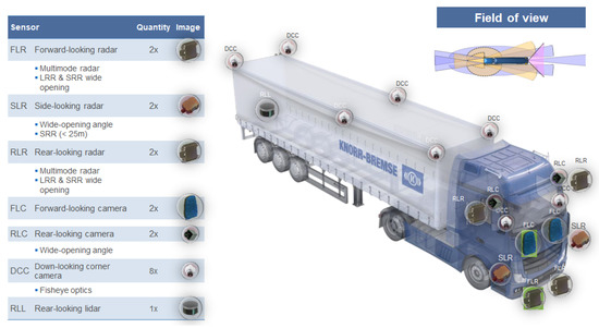
Figure 1.
The test vehicle highlighted with the installed sensors.
2.1.2. Decision Making
The information arriving from perception is abstract in nature: the sensor fusion provides an abstract world model in which we find a list of the detected peer vehicles and all of their parameters (e.g., relative distance, velocity, acceleration, detected side, width, length, class, etc.). The detected lanes/lines around the vehicle are also available for us to work with.
Also, the positions of all of these objects are transformed into a rectified world model which simplifies decision-making algorithms, as it eliminates certain trajectories that seemingly lead to a crash. Certainly, the curve of the lanes still needs to be considered due to the dynamic limits of the vehicles.
These preprocessed data are applied as the input to the risk estimation and scenario classification modules. The scenario classifier predicts traffic density for each lane. The risk estimator works on a discrete manoeuvre space and calculates risks for each of its points. The reason for the discretisation is that both the risk estimation and the behaviour planner algorithms run in an embedded environment with a limited computational capacity. They have to operate in real time; therefore, an arbitrarily fine quantisation of the manoeuvre space cannot be achieved.
The above-mentioned manoeuvre space defines manoeuvres as points on a horizontal plane in the ego vehicle’s reference system. The axes of this coordinate system are the longitudinal and lateral accelerations. The origin shows the acceleration values which are needed to maintain current speed and keep the vehicle in the lane. The discretisation of this manoeuvre space currently considers manoeuvre points, as shown in Figure 2.
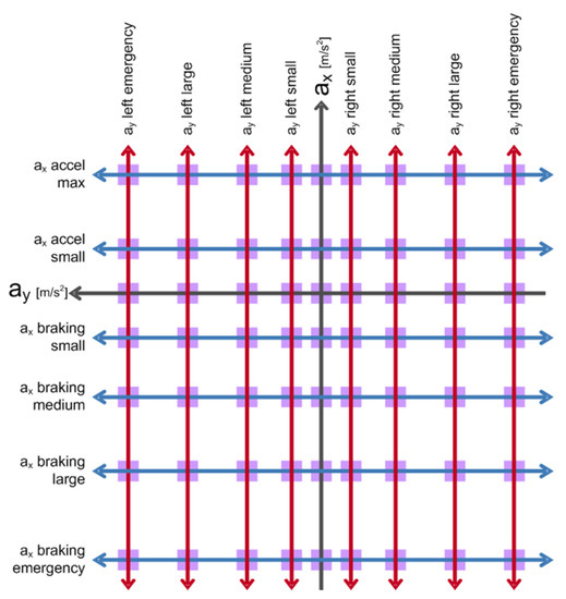
Figure 2.
The manoeuvre space which is defined in the ego’s reference system.
Both the classifier and the risk estimation module’s output is used by the behaviour planner, whose aim is to choose a point in the manoeuvre space defined in the car’s reference system which satisfies both the strategic and tactical objectives of the algorithm. The determined chain of actions thus define a trajectory which is created and executed by the lower-level actuation module.
2.2. Simulation Environment
The teaching, testing and evaluation of the developed algorithms require a simulation environment which can provide a large amount of traffic scenarios. For this purpose, we developed a simulator with a simple, two-dimensional viewer. The simulator has an interface that matches the perception module’s interface and also helps with the labelling task for the training data. This greatly facilitated our work due to the fact that we needed a simulator with a customised output; however, a sophisticated GUI was not required for our research. This proved to be exactly the opposite of what most of the automotive simulators could offer to us which were available for our use.
2.3. Situation Analysis
The goal of analysing the traffic situation around the ego is to recognise conditions and provide information beyond what the perception module offers, thus supporting the correct operation of the behaviour planner algorithm. For this, we utilise a risk estimator module which, in detail, assesses the degree of risk related to each of the previously presented 63 manoeuvre points in real time and a traffic density classifier.
2.3.1. Analysing Traffic Density
Classifying the level of traffic congestion on highways is a popular research area. Schnitman et al. [12] categorised the given situation into three classes—light, medium and heavy traffic—using the average crowd density and crowd speed as input parameters. They compared the performance of different classifiers, like the K-nearest neighbour, naive Bayes, support vector machine (SVM), and multilayer perceptron (MLP) algorithms. In their research, they achieved a 94.5% accuracy using neural networks.
This approach is relevant for our work, because human drivers adjust their driving attitude to the density level of the current traffic. For example, on an almost empty highway, drivers change lanes fairly quickly and frequently if needed. However, in a situation where the traffic is almost in a heavy congestion state, drivers usually stay in their lane, because passing one vehicle usually does not give a considerable strategic benefit regarding the navigational goal but creates an additional risk for all nearby vehicles.
In our research, we focused on investigating a traffic density classifier whose output is also used as an input for the behaviour planner algorithm. Beyond determining executable manoeuvres with an acceptable level of risk, another goal is to support behaviour planning with information that is one abstraction level higher than the data arriving from the environment perception module.
The parameters used as input to the classifier are a subset of the perception module’s output and the ego vehicle’s state vector. From these parameters, we calculate the following quantities for every traffic lane:
- the number of vehicles in the given lane per unit length,
- the average longitudinal velocity of the vehicles in the given lane,
- the average longitudinal acceleration of the vehicles in the given lane,
- and the average TIV parameter for the consecutive vehicles in the given lane.
TIV is an abbreviation for time-in-between-vehicles (or inter-vehicular time). It is a risk characterisation parameter used in the automotive field [13,14]. It can be calculated by , where is the speed of the vehicle behind, and D is the longitudinal distance between the vehicles following each other. See Figure 6 for the connection between the value of the parameter and the probability of collision.
The classifier analyses each traffic lane independently. The above-mentioned parameters are calculated for each moment. To filter out transient events, we use a 10 s wide moving window and sample the output data stream of the perception module with 100 ms intervals. We get 100 frames by this sampling. For constructing the feature vector used by the classifier, we combine the above 4 parameters of the last 100 sampled frames. This way, the classifier algorithm’s feature matrix is 400 wide. Our classifier categorises the traffic into five classes: empty, open flow, mild congestion, heavy congestion and “stop and go” traffic jam.
To acquire a teaching dataset, we used our simulation environment (mentioned in Section 2.2) that we developed for this purpose. All of dataset was hand-labelled with the help of the same environment.
According to the research of Porikli et al. [15], increasing the number of states to more than six is not beneficial, partly because of the subjective labelling assignment of the traffic condition by the human operator.
2.3.2. Risk Estimation
According to the most widespread definition in the automotive industry, the risk of an event is defined by the probability of its occurrence multiplied by the severity of the consequences [16]. In our case, a collision is the unwanted event, which we definitely wish to avoid; thus, probability is the primary factor influencing risk, and severity should only increase it. Because of these factors, we look for the risk of each manoeuvre in the form presented by Equation (1), where P stands for the probability and S stands for the severity.
As a result, a real number greater than or equal to zero is desired to indicate the risk. Figure 3 explains the meaning of the risk values we define in different ranges.
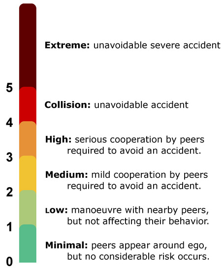
Figure 3.
Possible risk values and their meaning.
Concept
For a truly detailed situation analysis, a simulation along several trajectories seemed to have the best potential, though it has one major problem; namely, its high calculation demand. This issue also appears if a less complex vehicle model is used, as in our case, and the problem grows if the calculations need to be expanded in any angle. Our study is closely linked to the private sector; therefore, keeping hardware expenses low is a key aspect, too.
In this section, we present a risk estimation algorithm which has already proved to provide good results. However, its calculation demand makes it impossible to run the algorithm in real time on the test platform.
To overcome this obstacle, we applied machine learning within this neural network due to its ability to model non-linear problems. The above-mentioned algorithm serves as the ground truth. We used it for generating risk labels for the training and testing data.
Based on these considerations, we designed the system demonstrated in Figure 4.
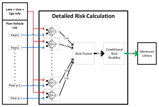
Figure 4.
Block scheme of the detailed risk calculation.
Input A subset of information provided by the environment perception interface and the state vector of the ego vehicle is used to calculate risk values at every time step.
Output After estimating the risk, we get a matrix, in which each element corresponds to a manoeuvre point. These values are then stored in a structure accessible to the subsequent behaviour planning algorithms.
Role of Neural Networks In Figure 4, we can see the same network multiple times with partly different inputs. Each of them is responsible for estimating the manoeuvre risks considering only one peer object.
Risk Fusion After a risk matrix is determined for each object, Risk Fusion merges them to a single matrix describing the whole situation. This operation is realised for each manoeuvre individually by Equation (2), which performs the calculation of p-norm on the vector of risks belonging to the different objects.
Conditional Risk Modifier In the last step, the algorithm might modify some of the risks considering simple conditions. Our solution investigates two aspects:
- If the foreseen distance of a lane’s end is getting significantly close to the ego, all risk values rise related to manoeuvres that are linked to that lane. Basically, the algorithm treats the end of a lane like a still standing object.
- All lane changing manoeuvres should have a risk value of at least one, thus preferring the lane keeping behaviour. As a result, a lane changing manoeuvre will only be performed if the behaviour planning algorithms can find significant benefits for it.
Calculating these conditions does not require a considerable amount of time, which is why it is not part of the labelling algorithm. All of the computational time-demanding analytical calculations are included in the labelling process and therefore substituted by neural networks. It is worth mentioning that training a neural network for a simpler task is much easier, and it leaves less chance for error.
Label Generation
Labelling the individual situations is carried out by a simulation algorithm in which various metrics of risk are used. Below, we specify the main components and steps of the algorithm:
Lateral Movement of Rear Objects First, in case the peer is in the ego’s lane and is following the ego, the algorithm applies a prediction that the peer vehicle is going to change its lane. Therefore, the object will be moved to the left or to the right by one lane, depending on its actual lateral speed. This is done because a faster vehicle coming from behind often overtakes us suddenly, and cutting in front of it could cause an accident, which we want to avoid.
Peer Motion Estimation Predicting the motion of peer vehicles is a topic on which separate research efforts are being carried out within the company. Currently, we use a simpler model for this task. We defined five manoeuvres: moving straight, following initial dynamics, heading to the left, heading to the right or staying in the same lane. We assign the most likely manoeuvre based on the weighted sum of the vehicle’s lateral speed, acceleration and relative position values. This manoeuvre is assumed for the object’s further movement.
Vehicle Model The ego and the peer vehicles are handled by the same simple physical model, where an object is a rectangle that is only able to perform translational movements. Each rectangle is described by its position, speed and acceleration vectors. During the simulation, these features are recalculated and updated step by step in order to complete the expected motion. The ego vehicle is simulated along all of the manoeuvres, in which nine different but similar trajectories are distinguished for each of them for a more precise approach.
Risk Components During the simulation, we look for component P and S of Equation (1) and note them continuously. To determine P, we applied the risk characterisation parameter time-to-collision (TTC) and inter-vehicular time (TIV), which are popular and frequently used in the automotive field [13,14].
TTC is a duration which shows how much time is left until a collision occurs should the objects advance at their current speed on their trajectories. Usually, is used to calculate it, where D is the longitudinal distance between the two vehicles; V and are the velocities of the ego and the peer vehicle, respectively. We choose the smallest of the TTC parameters calculated for the nine trajectories mentioned earlier, which all belong to the same manoeuvre (we run the TTC calculation in the lateral direction as well). Then, using the smallest one, we assign a probability of collision to the situation by applying the frequently used function shown in Figure 5. We only run the simulation to 10 s because, according to the function in Figure 5, the probability is zero for durations longer than that.
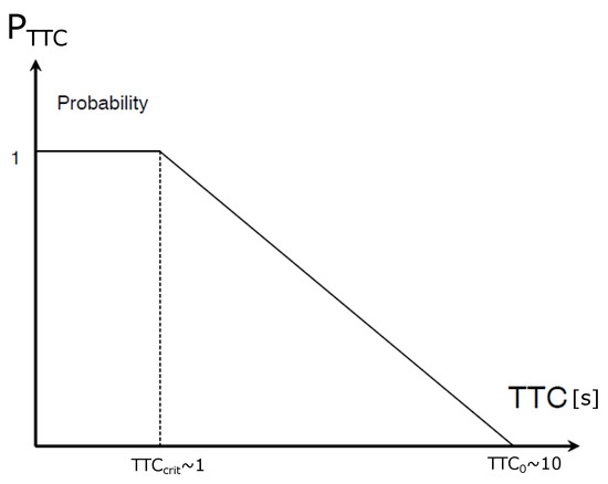
Figure 5.
Relationship between time-to-collision (TTC) and , which is the collision probability associated with TTC. shows an extreme time value of 1 second, when collision becomes highly likely ( is a common value for driver reaction time) [13].
We further modify the calculated with the function of the average of the smallest Euclidean distances between objects which could be measured along the nine trajectories.
As a result of this, we can reduce the risk of some special cases to a small extent when collision can be just avoided with a little luck. Based on this, the TTC part of component P of the risk is determined by Equation (3), where the scalar value serves to scale the above-defined values in relation to the risk.
Inter-vehicular time (TIV) is another parameter which indicates risk that TTC is not able to point out, e.g., vehicles following each other at dangerously close distance at almost the same speed. In this case, TTC is infinitely large, but TIV proves to be a more suitable indicator and can be calculated by , where is the speed of the rear vehicle, and D is the longitudinal distance between them. For TIV, the probability of collision is determined by the diagram shown in Figure 6.
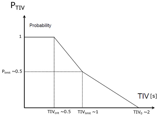
Figure 6.
Relationship between inter-vehicular time (TIV) and , which is the collision probability associated with TIV [13].
Our goal is to affect the risk using the TIV in every step of the simulation; since the risk is influenced by TIV, it can change instantaneously due to lane changing manoeuvres. Because of this, instead of the simple value, we use a weighted average, which is calculated by Equation (4)
where the value of t increases with the simulation step during the summation and not by units. The weight factor is determined by Equation (5):
We perform the above-mentioned accumulation of the TIV values on all the nine trajectories we discussed earlier for each manoeuvre. Then, we choose the minimum from the nine averages and determine the TIV-related collision possibility by the diagram shown in Figure 6. The TIV-related part of component P of the risk is calculated by Equation (6), where serves as a scaling parameter to the defined risk values, and likewise for .
We can accumulate component P with Equation (7) by considering the TIV- and TTC-related risks located along different dimensions.
We used method delta-v to determine component S, which was originally applied by Hobbs and Mills to evaluate the severity of human injuries [17]. Since then, this method has been used by several different studies [18]. For this, we need to determine the extent of the velocity change upon impact; then, by applying the extensively used curves [19], we can calculate the severity. The Abbreviated Injury Scale [20] (AIS) is a scale ranging from 1 to 6 which is used to indicate the severity of injuries. Equation (8) shows the probability of an injury with a severity of at least a level 3 on the AIS scale. This indicates the possibility of a clinically severe injury.
Due to the lack of observations, we can use only a simple model for the speed change. Currently, we take a relatively unfortunate case into account when the mass of one participant is insignificant compared with the other. In this case, the lighter vehicle suffers from the full speed difference upon impact. For this reason, the absolute value of the speed difference between the objects is registered for all nine trajectories during a frontal collision event in the simulation, then the maximum is chosen to calculate the severity of the collision using Equation (8), which approximates the blue curve in Figure 7 representing a frontal collision.
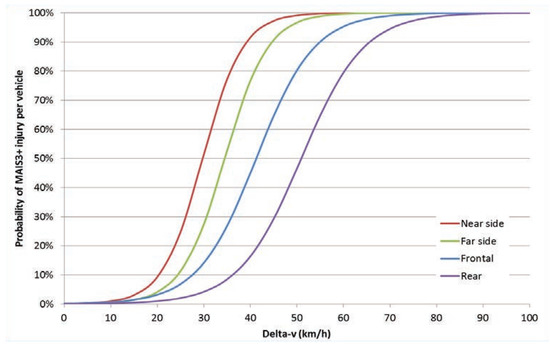
Figure 7.
Probability of severe injury against the suffered change in velocity for different types of collisions according to the measurements of Bahouth et al. (2014) [21].
Training Data
A large amount of data was required to teach the neural network to pay exceptional attention to the critical and most common situations. Several data sources were found to face the problem:
- previous real-world measurements,
- virtual measurements from different simulation environments,
- data generated from probability distributions and expert systems.
So far, we only dealt with data from the first two sources, and we got 300,000 training samples. Our simulation environment produced data with the same structure as the real-world measurements that we used. A sample, in this case, means the information of a time step (based on sensor data or simulation). The data that the neural network uses consist of the peer vehicles’ relative position, velocity and acceleration values (in both directions), their dimensions, the speed vector of the ego vehicle and some lane information.
Exploiting the last data source could be a future improvement, as it could best approximate real-world measurements and cover all of the state space.
Neural Network
While designing the structure of the network, the feed-forward multilayer perceptron (MLP) was chosen. The first tests already produced a converging net and a reasonably good accuracy. The configuration we eventually used is presented in Figure 8.
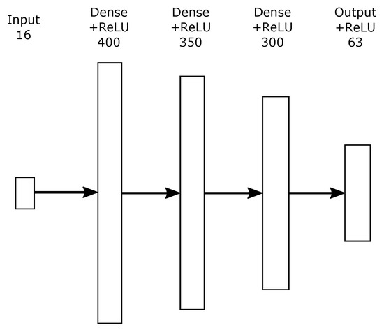
Figure 8.
Architecture of the presented neural network.
The architecture consists of three hidden layers, and it has 16 inputs. For input, the network uses the above-mentioned parameters for the given peer vehicle (position, velocity, acceleration, object length, object width), ego speed vector and certain lane information. We used ReLu [22] (rectified linear unit) activation functions on both the hidden layers and the output layer. Training used the Adam [23] optimisation algorithm with a mean-squared error (MSE) loss function.
We evaluated several different model configurations, some which are shown in Table 1. The second column shows the number of layers and the number of neurons for each layer. The epoch column reveals how many passes over the training dataset gave the best results.

Table 1.
Highlights of the tested neural network configurations.
2.4. Behaviour Planning
The behaviour planner algorithm works from environmental sensor data and from the outputs of the risk analysis and situation classifying modules. In summary, the available information in abstract form are the following:
- State vector of the vehicle
- -
- Longitudinal and lateral velocity
- -
- Longitudinal and lateral acceleration
- -
- Width and the length of the vehicle
- Environmental sensor data
- -
- Lane information
- -
- Line information (road markings)
- -
- Information about peer vehicles
- ∗
- Position
- ∗
- Longitudinal and lateral velocity
- ∗
- Longitudinal and lateral acceleration
- Output of the risk analysis module
- Output of the situation classifying module
The behaviour planner module chooses a point from the manoeuvre space, which is defined in the car’s reference system. Then, subsystems which are responsible for lower actuation plan a trajectory and execute it.
Reasons for Applying Probabilistic Inference
Algorithmizing behaviour planning as a task is not a trivial problem at all. It is not a simple controlling problem, as we need to understand the concept of driving at a much higher level. Human drivers subconsciously analyse the traffic situation while driving, and they make decisions based on their previous experiences, often relying on their intuitions. They try to estimate the movement of the peer vehicles based on the principle of trust; they change lanes reflexively. All of these manoeuvres are motivated by the goals they set: to travel from A to B as quickly or economically as possible while keeping their own and the others’ safety in mind. We have chosen probabilistic networks for handling the problem. The reasons for our decision are the following:
- Perceptions are uncertain: The environmental sensing module gives us uncertain information about the objects around us, so, practically, the input values of the algorithm are probabilistic variables, and they have expected values and deviations.
- All of the inputs of the task cannot be defined: If we want to implement driving with computer software, then we certainly do not know all the parameters that can influence the decisions. There are several reasons for this:
- -
- Laziness: Defining the complete system of causes and effects means too much work.
- -
- Theoretical ignorance: We do not know all of the parameters of driving as an algorithmizable task.
- -
- Practical ignorance: If we knew the whole rule-based system, there would still be several uncertainties surrounding the definition and measurement of the parameters.
- It is close to human thinking: With probabilistic networks, we can provide a solution to a high-level problem with a model which is similar to our thinking, and its graphic visualisation also makes the solution more straightforward.
- It reduces the number of parameters: Several known or unknown parameters can be replaced by a single probability variable. If the number of the parameters seems to be too low, the network can be extended until the operation seems right. The low number of parameters has several advantages:
- -
- Hidden parameters are also considered through the probabilities.
- -
- We do not complicate our algorithm with unnecessary parameters.
- -
- The calculation time can be significantly reduced in real-time applications.
Imagine that, initially, we decide on a lane change only on the basis of two questions: Is the lane next to us empty? Is somebody moving slowly in front of us? If the algorithm says that it is worthwhile to switch with 60% probability, and this is permitted by the rules and the traffic situation, then we made a decision with a very simplified model, but, in most of cases, this would prove to be good. If we add to this description additional variables, then we will be getting closer to the optimal solution, but we are still far from the practically impossible task of treating driving with all of the existing parameters. - The prediction appears in the algorithm: A human driver’s decision is often based on predicting the motions of the peer vehicles. These parameters can be easily grasped through probabilistic variables. Analysing the movement of the objects detected by the sensors, we can give estimates for the near future based on previous measurement data [14]. For example, if a car is passing by at a high speed, it is highly likely that it will not stop suddenly, but if there is a slowed vehicle in front of it, there is a high probability that it will also brake.
- We can make decisions based on probabilistic variables: If a probabilistic network is supplemented by additional node types, we can represent the decision problem with a so-called decision network. The decision network contains information about the state of the agent, and gives us the possible actions and the status that these actions will cause. From this point, the utility of the state can be treated as a problem of maximising a utility function.
Algorithm Design
Before detailing how to use probabilistic networks for behaviour planning, let us define two criteria for the competence of the module:
- The behaviour planner cannot make safety-critical decisions. This means that it can only select points defined in the manoeuvre space which were judged as safe by the risk analyser module (their risk is ranked as low or minimal).
- If the risk analysis module has assigned medium or higher risk values for all of the points in the manoeuvre space, then the decision of the algorithm cannot be based on the conditional probability tables learned before.
This means that the probabilistic network is confined to decisions that cannot endanger the vehicle and its environment. A manoeuvre that may have been wrongly selected can only be a mistake that hinders the achievement of the desired goal (for example, it results in slower progression).
Mathematical Tools To apply probabilistic conclusions, we need some mathematical knowledge about probability basics [24], probabilistic networks [25] and decision networks [26]. The summary of the needed mathematical apparatus is not the aim of this paper, and hereinafter we build on the basic knowledge of these topics.
Definition of Lane Change Options The risk analysis module assigns risk values to 63 different points, which are defined by longitudinal and lateral acceleration limits. Now, we want to reduce the number of these parameters to three: order probabilities for moving in our own lane and for changing traffic lanes to our right or left. This probability will mean the risk of changing. The first step is to divide the manoeuvre points into groups (or zones), as shown in Figure 9.
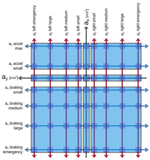
Figure 9.
Probability zones of lane changing risk.
So, the manoeuvre space was divided into nine parts based on two features:
- Longitudinal acceleration
- (a)
- Acceleration
- (b)
- Speed holding
- (c)
- Deceleration
- Lateral action
- (a)
- Lane changing to the left
- (b)
- Staying in our own lane
- (c)
- Lane changing to the right
Then, we want to assign a risk value to the zones, so we add the values in them using the following formula:
where n is the number of points in the zone.
In order to get probabilistic variables from the calculated risk values, we have to normalise them, which is performed for risk values assigned to a certain accident. The result has to be saturated to avoid values which are greater than one. With this operation, we practically get a probabilistic variable which characterises the risk of the zone.
As a result of the calculations we performed, there are three characteristic values per target traffic lane to which we can assign three simple Bayesian networks (one of them is shown in Figure 10). Teaching the networks results in a percentage value that characterises the probability of changing to (or staying in) the target lane. Do not forget that a dangerous decision cannot be made on this basis by the algorithm, because the output can only be a safe-risk manoeuvre.
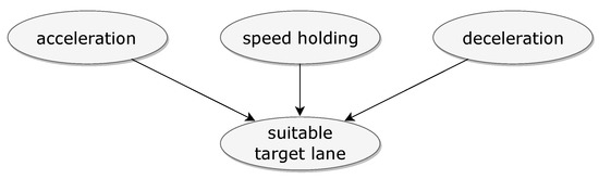
Figure 10.
Bayesian network for calculating the probability of changing to the target lane.
Apart from the above-discussed traffic-related reasons, lane changing can be blocked by traffic rules, so it is worth considering this as a direct input to a decision-making target function.
Definition of Lane Changing Needs In the previous step, we assigned a probability to the risk of the manoeuvre’s target lane, and this can tell us how likely it is to be safe to move in a given lane. Now, it is possible to determine lane changing needs [27]. We basically change lanes for two reasons:
- For navigational reasons
- In the hope of moving faster
Handling navigational needs is simple, as the information is available for each lane: whether it is suitable for accessing the set station or not, and when it stops being suitable. If this binary value is interpolated between zero and one (for example, along a straight line) on a given road section, then we can consider it a probabilistic variable, which gives us a percentage of the likelihood that a particular traffic lane is appropriate for us for navigation reasons.
Lane changing in the hope of moving faster is also not a very complicated problem. We know the maximum travel speed for every lane in the given road section, and we know our own speed. We see the vehicles around us and the vehicles passing by us; we know which lanes they use. Based on these data, we can calculate the average velocity of the lanes next to us. If we see that, for example, in the traffic lane on our left, there are no limitations to moving, then we can change lanes. If we would like to assign a probabilistic variable to this, we can select two points from which we can interpolate linearly:
- Assign 0% probability to speeds which are not greater than ours.
- Assign 100% probability to speeds which are larger by a given value (for example 15 km/h) than ours.
Measure the average speed of a traffic lane using a simple discrete filter, then determine our possible driving speed in the case of a lane change. The possible speed of travel will be the average speed of the lane or our maximum allowed speed (if the lane is moving faster). If the traffic lane is empty for a while, then the possible driving speed is our maximum allowed speed. The last task is to assign a probability to the speed value based on the above-mentioned rule.
For example, if a car is driving at 70 km/h in the outer lane while the average speed of the inner lane is 85 km/h, then it is theoretically 100% worth changing lanes. Note, however, that we are travelling in a heavy-duty commercial vehicle, which means we can only travel at 80 km/h, so the lane changing need, which is based on the hope of moving faster, can be characterised by a 67% probability, as shown in Figure 11.
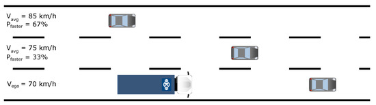
Figure 11.
Average driving speed and the probability of moving faster.
Structure of the Probabilistic Network The probabilistic variables, which were calculated with the simple methods enumerated so far, allow the construction of the simple Bayesian network mentioned in the introduction to this paper. Summarising the input points of the network:
- Suitability of target lanes which is based on risk calculation.
- Navigation-based lane changing needs.
- Lane changing needs, which can result in faster travelling.
Using the listed inputs, we can draw a conclusion per lane. If it is worth changing to it (or, in the case of our own lane, staying in it), then using the probabilities thus obtained, we can make the most appropriate decision. The constructed network is illustrated in Figure 12.
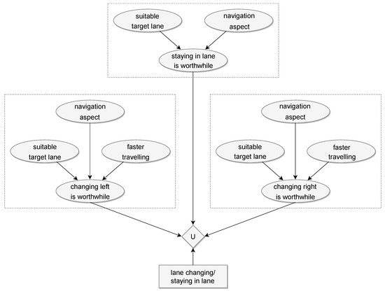
Figure 12.
The constructed simple Bayesian network.
As we can see, in our own lane, it does not make sense to define a probability variable for faster travelling based on the average velocity, because it would be a constant zero. It can also be seen that the network already contains a decision and utility node. The possible decisions are changing to a lane next to ours or staying in our own lane. The utility function selects the best lane for the moment based on the highest probability.
The output of the behaviour planner module should be a point in the manoeuvre space, but the network only defines the target lane. If we choose maximising speed as our goal, the choice is simple: we select the manoeuvre point from those belonging to the target lane which allows the maximum (still allowed) speed, with its risk value already acceptable for total security.
Operation of the Algorithm in Different Situations The probabilistic network seen in the previous point is quite simple, but it is able to handle the tasks defined in the introduction of this paper. Let us take a look at what we require from the algorithm in different situations and how our requirements are fulfilled.
- Movement in our own lane: In the case of heavy-duty commercial vehicles, the most significant part of travelling on the highway is characterised by this situation. The probabilistic network outlined in the previous part (if correctly trained) will mostly keep us in our own lane at the proper speed if it is appropriate for navigational purposes.
- Overtaking: Practically, overtaking means two consecutive lane changes. If the network decides to change and it sees that we can return to our original lane, then it will return. Of course, keeping to the right (or left, in the case of left-hand traffic) must be compelled with different weights in the utility function. Overtaking from the right and zigzag manoeuvres can be prevented by forbidding the lane changes to the right in the hope of moving faster.
- Lane changing: Lane changing differs from movement in our own lane in that it is not caused by traffic but is for a navigational reason, so it is not followed by returning to our original lane. Returning is prevented by a decrease in the original lane’s navigational probabilistic variable.
- Planning a danger avoidance manoeuvre: This situation is different from the others because, in this case, there are no points with an adequate security risk in the manoeuvre space. So, we cannot use the output of the probabilistic network, but we select the safest (or least dangerous) point.
Of course, the listed cases are considerably more complicated than presented, but since we do not make safety-critical decisions with the network, incorrectly selected manoeuvres can only cause slower movement or changing into lanes which are inappropriate for navigational reasons (as can occur with human driving). Reducing these errors can be guaranteed by providing adequate training data and by extending the very simple outlined network, which requires lots of testing, measurement and operating experience.
Training of the Probabilistic Network The word “training” is mentioned in the preceding paragraph, but the method of training is yet to be discussed. The probabilities are approximated with relative frequency during training, and, for this, we need tagged training data. Currently, we can imagine three possibilities for training:
- Tagging measurement data from a simulator and training the network.
- Tagging real measurements.
- Continuous learning during the operation of the system or learning the choices of a human driver.
In the first two cases, we tag the measurement data offline, and, in practice, we determine whether we want to change lanes or not. If we have a lot of data, the network will be able to handle previously unseen situations later. The third option assumes a functioning system that learns from its own mistakes, or it observes the decisions of its driver before turning on the self-driving mode. With this option, we have to be careful; although the behaviour planner module cannot make risky decisions, decisions can be bad in other respects. It is therefore worth limiting online learning by keeping the parameters within limits.
Another problem is that the lane changing option, while observing a human driver, is only detected by the system when the lane has been already changed, because we do not have any sensors in the driver’s head. That is why the first trained version of the probabilistic network will be created by manual tagging of simulator-generated or real-time measurements.
3. Results
The traffic density classification was done by a support vector machine algorithm. For 10,340 labelled data, we achieved 97% classification accuracy on the test dataset as a preliminary result. The SVM algorithm used a linear kernel, and we split the dataset into 30% test data and 70% training data.
For the risk estimator neural network, a mean-squared error (MSE) of 0.019 could be measured after 39 epochs, which means that the network hit the labelled risk values in the training dataset, on average, with a deviation of .
The results are consistent with our expectations regarding runtime: the neural network implementation usually finished execution in 2–3 ms, while the risk labelling algorithm required about 2 min on the same hardware (Lenovo T420, Core i5 2520M, 8 GB RAM) to complete an analysis of a situation. Although we think that our implementation could be further improved by the utilisation of GPGPU computing and algorithm optimisations, we would still lag behind from speeding up by nearly 4 orders of magnitude.
The presented behaviour planner module at this stage is still a concept that is operational in theory. We only performed practical tests with a small amount of training data already available to us. After testing, we surely need to extend the network with additional variables, such as driving comfort, outputs of the situation classification module or the optimisation of consumption. There are still other options for manoeuvres. For example, if we would like to change lanes, we can indicate it using the indicator lights. If the peer vehicles react properly, then the previously unmanageable manoeuvre becomes safe.
4. Discussion
During our research, we investigated the use of neural networks for real-time risk estimation, support vector machines for traffic situation classification and Bayesian and decision networks for making decisions about lane changing.
For traffic density classification, we definitely need to extend our training dataset in the future. Due to the high dimensionality of the feature space used as input, we are also going to investigate the application of dimensionality reduction algorithms like PCA (principal component analysis), which can show us if we need to improve our concept regarding the input parameters.
The achieved accuracy with the neural network is promising, and it suggests that we can benefit from the real-time capability of neural networks while getting results that are almost as good as the analytical calculations which serve as the ground truth for labelling the training data of the neural network. This means that the trained net could make the right decisions, even if it encounters situations for which it has not been trained explicitly with the training set.
In the future, we plan to increase the level of depth of our labelling algorithm for the risk estimation, as well as use more complex vehicle models and peer motion estimation. We are also going to investigate other network structures and improve the accuracy of the trained network by using different hyperparameter optimisation algorithms.
For the decision networks, we would like to illustrate the operation of the implemented algorithms through a simulation example (see Figure 13).
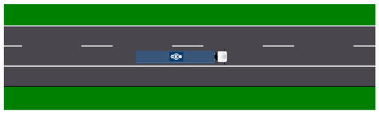
Figure 13.
Initial moment of the simulation.
The possibility of changing to the left lane is steadily decreasing as the passenger car 50 m behind us at the moment of departure approaches us at high speed. Meanwhile, another important event can be observed: we start to catch up with the slower truck. The traffic situation at the end of the 2nd second is shown in Figure 14.
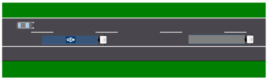
Figure 14.
The 2nd second of the simulation.
By the time the car is next to us, the system has had to slow down our vehicle. The speed-related probability was higher than zero, but we were forced to stay behind the other truck in our lane because of the busy left lane. The events of the 3rd second are shown in Figure 15.
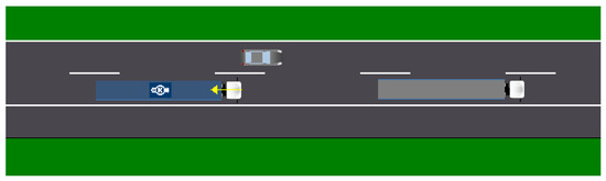
Figure 15.
The 3rd second of the simulation.
By the end of the 5th second, the car is in the position shown in Figure 16. Up to this point, we have slowed down to the speed of the truck ahead (which is 66 km/h). This (considering the status of the left lane) means that the probability of faster progress is 93%. Due to the possibility of moving faster and the obstacle in front of us, the probability of suitability of the left lane is also slightly higher than our lane’s (left: 88%, ours: 77%). The decision is made: we start to overtake.
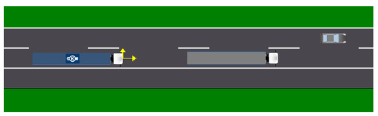
Figure 16.
The 5th second of the simulation.
In the 11th second, we are already in the middle of overtaking. The system cannot make any decisions other than continuing to overtake: there is no road to the left, and there is the truck to the right. This means that only our own lane does not have a zero suitability probability value: specifically, its value is 76%. The events are illustrated in Figure 17.
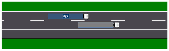
Figure 17.
The 11th second of the simulation.
The overtaking ends in the 20th second of the simulation, which can be seen in Figure 18. The system detects that the right lane is empty, so it takes the necessary steps and changes the lane.
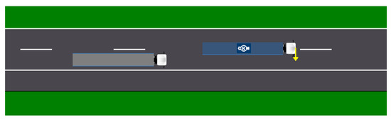
Figure 18.
The 20th second of the simulation.
For the training, we used 25–30 steps of situations, and some moments from these sequences served as training data for the probabilistic network. Each simulation takes a few tens of seconds, and the time depends on the situation. It takes a few seconds to test a security stop, but overtaking can take up to half a minute.
Based on our experience, the algorithm still needs refinement. Based on the current training, we believe the decisions are too cautious. The most typical behaviour is staying in our own lane, even if we can safely change lanes and need to do so. It is difficult to define an exact number for the efficiency of the algorithm; most of all, we can judge on the basis of how naturally it drove. Looking at this aspect, we have come to the conclusion that vehicle behaviour can be accused of being excessively cautious.
Phenomena other than natural, which need refinement, can be found in the example presented in this section. In the screenshots of overtaking, you can see that the vehicle is approaching the one ahead of it, picking up its speed, and, when it becomes safe, it starts to overtake. In this situation, the expectation would be to get closer to the object with a less powerful but previously started slowdown. During further refinement, we will comprehensively examine the impact of teaching data on such situations, and we will also reconsider the structure of the net.
While running the tests, because of the basic principles set out in the theoretical structure of the model (we do not make security-critical decisions with probabilistic conclusions), accidents have not occurred in situations that were realistic to handle. Of course, we also made situations when the accident cannot be avoided. The efficiency of avoiding emergencies depends on the accuracy of the output of the risk analysis module. We have seen the decision making of the behaviour planner module in such cases: it always strives to minimise risk.
Another requirement for the algorithm is real-time operation, and we have succeeded in doing so. The simulator runtime, along with risk analysis, situation classification and behaviour planning is roughly a third of the duration of the simulation. Staying with the above example, a 25 s situation means 8.41 s in a desktop environment.
Author Contributions
Conceptualization, B.D., G.L. and G.H.; methodology, B.D., G.L. and G.H.; software, B.D., G.L. and G.H.; writing—original draft preparation, B.D., G.L. and G.H.; writing—review and editing, B.D., G.L. and G.H.
Funding
The research reported in this paper was supported by the Higher Education Excellence Program of the Ministry of Human Capacities in the frame of Artificial Intelligence research area of Budapest University of Technology and Economics (BME FIKP-MI/SC). This paper was also supported by Pro Progressio Foundation.
Acknowledgments
We would like to express our gratitude to our colleagues Zoltan Gyurkó, Kornél Straub and Csaba Horváth at Knorr-Bremse Fékrendszerek Kft. for the regular meetings and consultations, without whose help this paper could not have been written. Special thanks to Domokos Kiss, who helped our research as our university consultant.
Conflicts of Interest
The authors declare no conflict of interest.
References
- SAE International. Taxonomy and Definitions for Terms Related to Driving Automation Systems for On-Road Motor Vehicles; SAE International: Warrendale, PA, USA, 2016. [Google Scholar]
- Lefèvre, S.; Vasquez, D.; Laugier, C. A survey on motion prediction and risk assessment for intelligent vehicles. ROBOMECH J. 2014, 1. [Google Scholar] [CrossRef]
- Lytrivis, P.; Thomaidis, G.; Amditis, A. Cooperative path prediction in vehicular environments. In Proceedings of the 2008 11th International IEEE Conference on Intelligent Transportation Systems, Beijing, China, 12–15 October 2008; pp. 803–808. [Google Scholar]
- Aoude, G.S.; Luders, B.D.; Lee, K.K.H.; Levine, D.S.; How, J.P. Threat assessment design for driver assistance system at intersections. In Proceedings of the 13th International IEEE Conference on Intelligent Transportation Systems, Funchal, Portugal, 19–22 September 2010; pp. 1855–1862. [Google Scholar]
- Ammoun, S.; Nashashibi, F. Real time trajectory prediction for collision risk estimation between vehicles. In Proceedings of the 2009 IEEE 5th International Conference on Intelligent Computer Communication and Processing, Cluj-Napoca, Romania, 27–29 August 2009; pp. 417–442. [Google Scholar]
- Batz, T.; Watson, K.; Beyerer, J. Recognition of dangerous situations within a cooperative group of vehicles. In Proceedings of the 2009 IEEE Intelligent Vehicles Symposium, Xi’an, China, 3–5 June 2009; pp. 907–912. [Google Scholar]
- Kaempchen, N.; Schiele, B.; Dietmayer, K. Situation assessment of an autonomous emergency brake for arbitrary vehicle-to-vehicle collision scenarios. IEEE Trans. Intell. Transp. Syst. 2009, 10, 678–687. [Google Scholar] [CrossRef]
- Vanholme, B.; Gruyer, D.; Lusetti, B.; Glaser, S.; Mammar, S. Highly Automated Driving on Highways based on Legal Safety. Ph.D. Dissertation, University of Evry-Val-d’Essonne, Évry, France, 2012. [Google Scholar]
- Ulbrich, S.; Maurer, M. Probabilistic Online POMDP Decision Making for Lane Changes in Fully Automated Driving. In Proceedings of the 16th International IEEE Conference on Intelligent Transportation Systems, The Hague, The Netherlands, 6–9 October 2013. [Google Scholar]
- Wei, J.; Dolan, J.M.; Litkouhi, B. A Prediction- and Cost Function-Based Algorithm for Robust Autonomous Freeway Driving. In Proceedings of the 2010 IEEE Intelligent Vehicles Symposium University of California, San Diego, CA, USA, 21–24 June 2010. [Google Scholar]
- Ulbrich, S.; Maurer, M. Towards Tactical Lane Change Behavior Planning for Automated Vehicles. In Proceedings of the IEEE 18th International Conference on Intelligent Transportation Systems, Las Palmas, Spain, 15–18 September 2015. [Google Scholar]
- Schnitman, L.; Sobral, A.; Oliveira, L. Highway traffic congestion classification using holistic properties. In Proceedings of the 10th IASTED International Conference on Signal Processing, Pattern Recognition and Applications, Innsbruck, Austria, 12–14 February 2013; Volume 798. [Google Scholar]
- Glaser, S.; Vanholme, B.; Mammar, S.; Gruyer, D.; Nouveliere, L. Maneuver-based trajectory planning for highly autonomous vehicles on real road with traffic and driver interaction. IEEE Trans. Intell. Transp. Syst. 2010, 11, 589–606. [Google Scholar] [CrossRef]
- Bahram, M.; Wolf, A.; Aeberhard, M.; Wollherr, D. A prediction-based reactive driving strategy for highly automated driving function on freeways. In Proceedings of the 2014 IEEE Intelligent Vehicles Symposium Proceedings, Dearborn, MI, USA, 8–11 June 2014; pp. 400–406. [Google Scholar]
- Porikli, F.; Li, X. Traffic congestion estimation using HMM models without vehicle tracking. In Proceedings of the IEEE Intelligent Vehicles Symposium, Parma, Italy, 14–17 June 2004; pp. 188–193. [Google Scholar] [CrossRef]
- Hansson, S.O. Risk. In The Stanford Encyclopedia of Philosophy; Zalta, M.N., Ed.; Etaphysics Research Lab, Stanford University: Stanford, CA, USA, 2018. [Google Scholar]
- Mills, P.J.; Hobbs, C.A. The Probability of Injury to Car Occupants in Frontal and Side Impacts; SAE Technical Paper; SAE International: Warrendale, PA, USA, 1984; Volume 10. [Google Scholar]
- Pride, R.; Giddings, D.; Richens, D.; McNally, D.S. The sensitivity of the calculation of delta-v to vehicle and impact parameters. Accid. Anal. Prev. 2013, 55, 144–153. [Google Scholar] [CrossRef] [PubMed][Green Version]
- Jurewicz, C.; Sobhani, A.; Woolley, J.; Dutschke, J.; Corben, B. Exploration of vehicle impact speed—Injury severity relationships for application in safer road design. Transp. Res. Procedia 2016, 14, 4247–4256. [Google Scholar] [CrossRef]
- Gennarelli, T.A.; Wodzin, E. The Abbreviated Injury Scale; American Association for Automotive Medicine: Des Plaines, IL, USA, 2005. [Google Scholar]
- Bahouth, G.; Graygo, J.; Digges, K.; Schulman, C.; Baur, P. The benefits and tradeoffs for varied high-severity injury risk thresholds for advanced automatic crash notification systems. Traffic Inj. Prev. 2014, 15 (Suppl. 1), S134–S140. [Google Scholar] [CrossRef] [PubMed]
- LeCun, Y.; Bengio, Y.; Hinton, G. Deep learning. Nature 2015, 521, 436–444. [Google Scholar] [CrossRef] [PubMed]
- Kingma, D.P.; Ba, J. Adam: A Method for Stochastic Optimization. In Proceedings of the International Conference on Learning Representations, San Diego, CA, USA, 7–9 May 2015. [Google Scholar]
- Vetier, A. Probability Theory; Muegyetemi Kiado: Budapest, Hungary, 2008. [Google Scholar]
- Bayes Server Learning Center. Available online: https://www.bayesserver.com/ (accessed on 15 November 2018).
- Stuart, R.; Peter, N. Artificial Intelligence. A Modern Approach, 2nd ed.; Pearson Education Inc., Prentice Hall: Upper Saddle River, NJ, USA, 2003; p. 07458. ISBN 0137903952. [Google Scholar]
- Nilsson, J.; Silvlin, J.; Brannstrom, M.; Coelingh, E.; Fredriksson, J. If, When, and How to Perform Lane Change Maneuvers on Highways. IEEE Intell. Transp. Syst. Mag. 2016, 8, 68–78. [Google Scholar] [CrossRef]
© 2019 by the authors. Licensee MDPI, Basel, Switzerland. This article is an open access article distributed under the terms and conditions of the Creative Commons Attribution (CC BY) license (http://creativecommons.org/licenses/by/4.0/).