Fighting CPS Complexity by Component-Based Software Development of Multi-Mode Systems

Abstract

Growing software complexity is an increasing challenge for the software development of modern cyber-physical systems. A classical strategy for taming this complexity is to partition system behaviors into different operational modes specified at design time. Such a multi-mode system can change behavior by switching between modes at run-time. A complementary approach for reducing software complexity is provided by component-based software engineering (CBSE), which reduces complexity by building systems from composable, reusable and independently developed software components. CBSE and the multi-mode approach are fundamentally conflicting in that component-based development conceptually is a bottom-up approach, whereas partitioning systems into operational modes is a top-down approach with its starting point from a system-wide perspective. In this article, we show that it is possible to combine and integrate these two fundamentally conflicting approaches. The key to simultaneously benefiting from the advantages of both approaches lies in the introduction of a hierarchical mode concept that provides a conceptual linkage between the bottom-up component-based approach and system level modes. As a result, systems including modes can be developed from reusable mode-aware components. The conceptual drawback of the approach—the need for extensive message exchange between components to coordinate mode-switches—is eliminated by an algorithm that collapses the component hierarchy and thereby eliminates the need for inter-component coordination. As this algorithm is used from the design to implementation level (“compilation”), the CBSE design flexibility can be combined with efficiently implemented mode handling, thereby providing the complexity reduction of both approaches, without inducing any additional design or run-time costs. At the more specific level, this article presents (1) a mode mapping mechanism that formally specifies the mode relation between composable multi-mode components and (2) a mode transformation technique that transforms component modes to system-wide modes to achieve efficient implementation.

1. Introduction

Growing software complexity is posing a challenge for the design of cyber-physical systems (CPS) [1]. Complexity related to CPS software is multifaceted, including specific requirements related to extra functional properties such as functional safety, resilience and timeliness. There is additionally a trade-off between the different aspects of complexity, e.g., added complexity at design-time can reduce complexity at run-time and vice versa. A key issue in making such trade-offs is the risk implied by different choices; and risks have to be balanced against benefits. For companies, this is a reality even for safety-critical systems regulated by safety standards. As a result, to maximize business benefits, it is standard practice for many companies to make a minimal, but sufficient, effort to comply with applicable regulation.

At the technological level, there are approaches developed to reduce complexity throughout the system life-cycle. Combining such approaches can potentially reduce the overall life-cycle complexity, but approaches are not always compatible, and each of them introduces both benefits and costs. This article presents the integration of two such approaches: multi-mode systems and component-based software engineering, which both provide composability, but are targeting different life-cycle phases. A specific challenge in combining the two is that they are conceptually incompatible, in the sense that component-based development is a bottom-up approach, whereas partitioning systems into operational modes is a top-down approach with its starting point from a system-wide perspective. Still, we are able to successfully integrate them in a single framework of multi-mode components, thereby providing the combined benefits of both, while being able to reduce costs to acceptable levels. These approaches, introduced below, are primarily focusing on the design, configuration and run-time phases of the system life-cycle, although they do have important implications also for the maintenance phase. Furthermore, other dimensions of complexity are affected by the considered technologies, including organizational complexity, as both component-based software engineering (CBSE) and the multi-mode approach provide a basis not only for system partitioning, but also for partitioning of the design activities, implying that the distribution of the design tasks to different departments or even different organizations are facilitated. A further implication of the enabled partitioning and inherent clearly-defined interfaces is that the approaches could scale also to systems-of-systems (SoS), e.g., different components or modes can correspond to different systems in an SoS.

1.1. Multi-Mode Systems

A common practice to manage software complexity is to partition system behaviors into different mutually-exclusive operational modes so that each mode corresponds to a specific system behavior. A multi-mode system [2] changes behavior by switching modes. A typical example is the control software of an airplane, which runs in different modes such as taking off, flight and landing. Multi-mode systems have also been motivated by many other reasons:

• Faster development: system behavior for different modes can be designed and tested in parallel.
• Diversified functionalities due to multiple modes.
• Enable adaptivity by mode-switch.
• Efficient resource usage: optimized resource reservation for each mode instead of fixed resource reservation.
• Fault tolerance: safety-critical systems can switch to a safe mode in case of a fault.
• Extensibility and scalability: it is flexible to add new modes and integrate them with an existing system.

1.2. Component-Based Software Engineering

As a complementary approach to multi-mode systems, CBSE [3] advocates the reuse of independently developed software components as a promising technique for the development of complex software systems. The success of CBSE has been evidenced by a variety of component models proposed both in industry and academia [4,5]. CBSE suggests software modularity and reusability to facilitate the development of high-quality software. For instance, different functional modules or even subsystems of the control software of an airplane can be encapsulated into reusable software components that can be reused multiple times for the same system or for other systems in the same software product line.

Applying CBSE in multi-mode systems or the other way around has been a largely unexplored research area, possibly because multi-mode systems and CBSE are fundamentally conflicting in the sense that the former traditionally is a top-down approach, whereas the latter is a bottom-up approach. Despite this apparent conflict, our research goal in this article is to combine these approaches and benefit from the advantages of both multi-mode systems and CBSE. Hence, we propose component-based software development of multi-mode systems, characterized by the independent development and reuse of multi-mode components (i.e., components that can run in multiple modes).

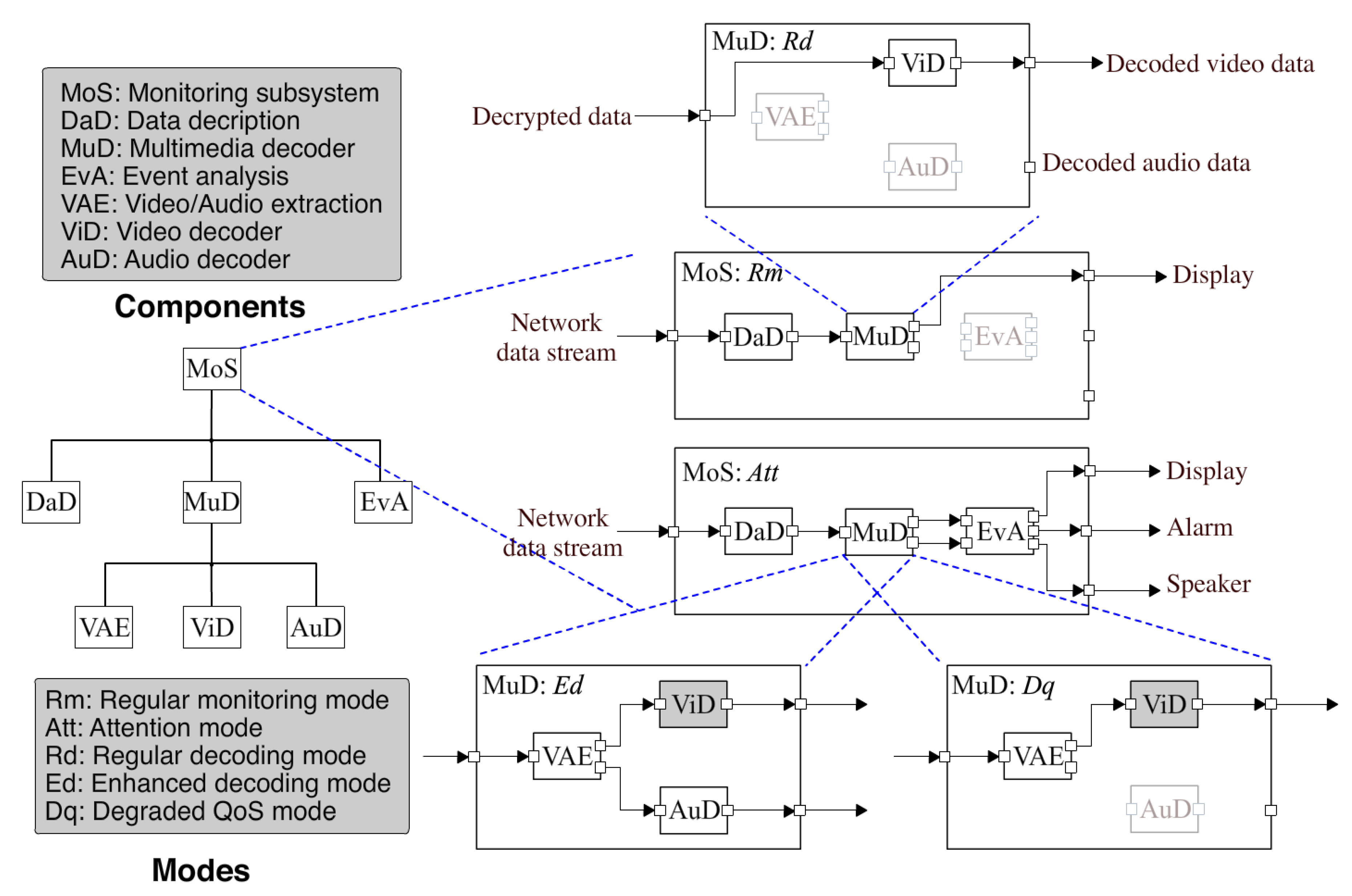
1.3. A Guiding Example

As a guiding example, consider a proof-of-concept healthcare monitoring system. The system consists of two subsystems: a data acquisition subsystem and a monitoring subsystem. The data acquisition subsystem uses cameras and microphones to collect video and audio data from a ward or a private home. Video and audio data are separately encoded and encrypted before transmission. The monitoring subsystem decrypts and decodes data that it receives and reports them to the health center. The monitoring subsystem also includes an alarm that is triggered when the person being monitored encounters a dangerous situation, such as falling or suffering from a heart attack.

Our focus is on the software architecture of the monitoring subsystem (MoS), which is composed of multi-mode components. Figure 1 illustrates the component hierarchy of the system on the left and component connections on the right. The system can be considered as a top-level component MoS with three subcomponents: DaD for data decryption, the multimedia decoder MuD and EvA for event analysis. Due to the tree structure of the component hierarchy, DaD, MuD and EvA are also called the children of MoS, which consequently is their parent. The system can run in two different modes: regular monitoring mode (denoted as Rm) and attention mode (denoted as Att).

The default mode of MoS is Rm when nothing special happens. To save resource in this mode, a fast video encoding/decoding algorithm can be selected and only low resolution video is transmitted to keep low CPU and bandwidth usage. Shown in Figure 1, small squares denote the input and output ports of a component, while each arrow that connects two ports denotes the data flow. Basically, each component has input data coming from its input ports, processes the data and provides output data at its output ports. Such a pipes and filters architectural style is fairly common for multimedia applications. The video data are first decrypted by DaD and subsequently decoded by MuD, which sends the decoded video data to the display in the health center. Represented by the dimmed color, EvA is deactivated when MoS runs in Rm. Meanwhile, DaD runs in a regular mode R1 and MuD runs in a regular decoding mode Rd. MuD has three subcomponents: VAE for video/audio extraction, a video decoder, ViD, and an audio decoder, AuD. ViD is the only activated subcomponent running in a regular video decoding mode Rvd as MuD runs in Rd. VAE and AuD are deactivated as shown in Figure 1 because no audio data are transmitted.

When the data acquisition subsystem detects an accident, both subsystems will switch to an attention mode Att to raise the attention of the health center. The network load is increased due to transmission of video data with higher quality and audio data. Component EvA becomes activated running in a regular mode R2, to analyze the detected event and trigger an alarm when necessary. MuD starts to run in enhanced decoding mode Ed, where all its subcomponents (VAE, ViD, AuD) are activated and a different video encoding/decoding algorithm is used to support higher resolution video. VAE runs in a regular mode R3 to separate decrypted video and audio data and send them to ViD and AuD, respectively. Represented by grey color in Figure 1, ViD runs in an enhanced video decoding mode Evd with a different video decoding algorithm for high quality video. AuD runs in a regular audio decoding mode Rad. In the case of poor network condition, MuD switches to a degraded QoS mode Dq, where the transmission of audio data is terminated to keep video quality, which is considered to be more important. Therefore, AuD becomes deactivated.

We distinguish two types of components in the monitoring subsystem: primitive components and composite components. DaD, EvA, VAE, ViD and AuD are primitive components, which are directly implemented by code, while MoS and MuD are composite components composed by other components. What makes this system distinctive compared with traditional component-based systems is its constitution of multi-mode components, i.e., components that can run in different modes at run-time. The system in Figure 1 indicates a clear mapping between the modes of different components. Such a mapping is summarized in

Table 1. Mode mappings.

(a) Mode Mapping of MoS				(b) Mode Mapping of MuD
Component	Modes			Component	Modes
MoS	Rm	Att		MuD	Rd	Ed	Dq
DaD	R1			VAE	$Deactivated$	R3
MuD	Rd	Ed	Dq	ViD	Rvd	Evd
EvA	$Deactivated$	R2		AuD	$Deactivated$	Rad	$Deactivated$

, where modes in the same column are mapped to each other for the composite components MoS and MuD. For instance, when MoS runs in mode Att, DaD must run in R1, MuD can run in either Ed or Dq and EvA must run in R2. Even already, this simple example signifies the power of building multi-mode systems with multi-mode components, which has the potential to enrich system architectural variability at all levels. Since multi-mode components still comply with component-based development, the overall software design complexity is decoupled into building multi-mode components at different levels, thereby making the growing software complexity manageable.

1.4. Contributions

In achieving component-based software development of multi-mode systems, this article includes two key contributions. First, we propose a formal mode mapping description in the form of mode mapping automata (MMA) that specifies how the modes of a composite component are mapped to the modes of its subcomponents. The MMA presented in this article partially builds on the MMA initially proposed in [6], which is here substantially refined and extended. Mode mapping elegantly links modes and software component reuse. The hierarchical composition of multi-mode components easily allows one to build multi-mode systems with multi-mode behaviors at various levels. A potential drawback of this approach is the run-time overhead due to inter-component communication for coordination of the mode-switches of different components. To eliminate this run-time drawback, while still being able to design systems from reusable multi-mode components, we introduce a mode transformation technique as our second contribution. This technique transforms component modes to system-wide modes to optimize the implementation. This is obtained by flattening the hierarchical structure of component modes mapped at different levels. Mode transformation can be included in the mapping from the design to implementation level (“compilation”), after the mode mappings of all composite components in a system have been specified. An initial version of the mode transformation technique is presented in [7].

The rest of this article is structured as follows: Section 2 elaborates on the composition of multi-mode components and the mode mapping mechanism. Section 3 presents the mode transformation technique. Related work is reviewed in Section 4. Finally, Section 5 concludes the article and discusses some future work.

2. The Composition of Multi-Mode Components

As an essential step in the composition of multi-mode components, mode mapping unambiguously specifies the mode relation between different multi-mode components at design time. This section highlights the essential properties of multi-mode components and the motivation of mode mapping, followed by a thorough explanation of MMA, i.e., a formal description of mode mapping.

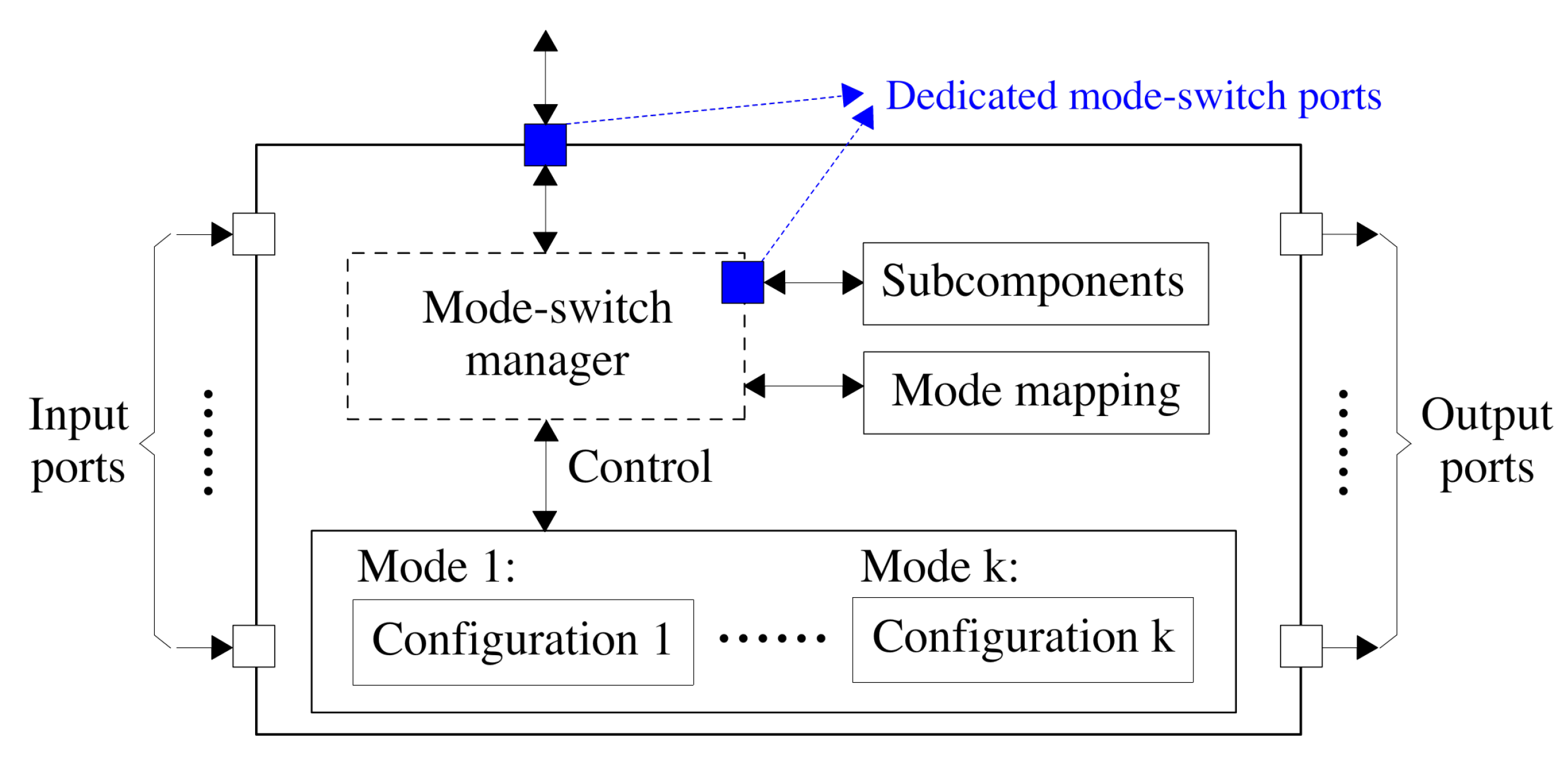
2.1. Multi-Mode Components and Mode Mapping

A multi-mode component supports multiple modes and has a unique configuration defined for each mode. Figure 2 illustrates the key properties of a reusable multi-mode component. The configuration for each mode relies on various factors. For instance, a multi-mode primitive component may have different mode-specific behaviors for different modes; while a multi-mode composite component may have a different set of subcomponents activated depending on its mode.

A multi-mode component can switch between certain modes at run-time, either on its own initiative or as the result of a request by another component. A mode-switch leads to the reconfiguration of the component by changing its configuration in the current mode to a new configuration in the target mode. A local mode-switch manager is used to handle the mode-switch of a multi-mode component. By having such a mode-switch manager in each component, a multi-mode component is able to exchange mode information with its parent and subcomponents via dedicated mode-switch ports (the blue ports in Figure 2) during a mode-switch, even without knowing the global mode information. These mode-switch ports do not deal with input or output data going through the component. Instead, they are only used for mode-switch coordination between a composite component and its subcomponents. Therefore, each mode-switch port is bidirectional, which allows mode-switch signals to be transmitted in both directions. For instance, in the guiding example presented in Section 1.3, when an accident is detected, MoS will switch from Rm to Att. Meanwhile, the mode-switch manager of MoS will send a signal to its subcomponents DaD, MuD and EvA, requesting them to switch mode based on the mode mapping defined in Table 1 (a). The mode-switch managers of different components are jointly responsible for propagating a mode-switch event to the affected components, keeping mode consistency between components and coordinating the mode-switches of different components. Designing the mode-switch manager is out of the scope of this article. We have previously developed distributed mode-switch algorithms [8,9] running in the mode-switch manager for the cooperative mode-switch of different components. Here, our focus is on mode mapping, also shown in Figure 2.

Since we assume that multi-mode components are independently developed, they typically support different numbers of modes and name them differently. It is necessary to specify the relation between the modes of different components at design-time without ambiguity. Such a specification is called mode mapping. To ensure reusability, the mode mapping must never violate the following principles:

• A primitive component only knows own mode’s information such as supported modes, initial mode and the current mode of itself.
• A composite component knows the mode information of itself and its immediate subcomponents.

The principles imply that mode mapping should be managed by each composite component, not by its subcomponents. A primitive component requires no mode mapping. The mode mapping defined in Table 1 is simple and intuitive; however, it is incapable of showing the initial mode of each component, which component initiates a mode-switch and the exact mode-switch of each individual component due to a mode-switch event. For example, when MoS switches from Rm to Att, according to Table 1 (a), MuD may switch to either Ed or Dq. Such non-determinism can be eliminated by specifying either Ed or Dq as the default new mode of MuD for this particular mode-switch scenario. To be able to formally specify all types of mode mapping rules, we propose a more powerful representation: the mode mapping automata.

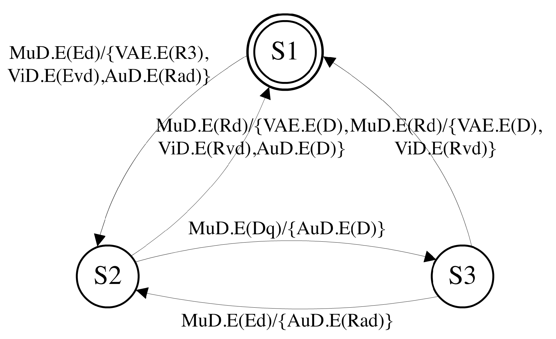
2.2. Mode Mapping Automata

Let c be a composite component with ${\mathcal{SC}}_c$ being the set of subcomponents of c and $P_c$ being the parent of c. When c is running in one of its supported modes, it should always know its current mode and the current modes of all $c_i\in {\mathcal{SC}}_c$ by its mode mapping. Moreover, whenever the mode-switch manager of c notices the mode-switch of $c_i\in {\mathcal{SC}}_c\cup \{c\}$, it will refer to the mode mapping, which should tell which other components among ${\mathcal{SC}}_c\cup \{c\}\setminus \{c_i\}$ should also switch mode as a consequence, as well as the new modes of these components.

The complete mode mapping of c can be formally presented by a set of MMA, which consists of one mode mapping automaton of c (denoted as ${MMA}_c^s$) and one MMA of each subcomponent $c_i\in {\mathcal{SC}}_c$ (denoted as ${MMA}_{c_i}^c$). Here, we call ${MMA}_c^s$ a self-MMA and ${MMA}_{c_i}^c$ a child MMA.

As an example, Figure 3 presents the set of MMA of the component MuD in Figure 1, including a self-MMA (${MMA}_{\mathit{MuD}}^s$) and three child MMA (${MMA}_{\mathit{VAE}}^c$, ${MMA}_{\mathit{ViD}}^c$ and ${MMA}_{\mathit{AuD}}^c$). These MMA are hierarchically organized in the same way as the corresponding components. Each MMA can receive and emit internal or external signals. Internal signals are used to synchronize the pair of the self-MMA and its child MMA while external signals interact with its local mode-switch manager for requesting and returning mode mapping results.

An external signal indicates that a component is requested to switch to a particular mode. We use $x.E(y)$ to denote an external signal asking ${MMA}_x$, which is either a self-MMA or a child MMA, to switch to mode y. An internal signal is sent either from a self-MMA to a child MMA or from a child MMA to the self-MMA. A self-MMA only sends an internal signal to a child MMA if the current mode-switch event requires the mode-switch of the corresponding subcomponent. The self-MMA decides the new mode of this subcomponent. We use $x.I(y)$ to denote an internal signal emitted by a self-MMA to the child MMA ${MMA}_x^c$, asking the subcomponent x to switch to mode y. A child MMA can also send an internal signal to the self-MMA. This implies that the corresponding subcomponent is requesting a mode-switch. Since mode mapping is always determined by the self-MMA, the internal signal from a child MMA only needs to contain the current mode and new mode of the corresponding subcomponent. We use $x.I(z\to y)$ to denote an internal signal emitted by a child MMA ${MMA}_x^c$ that requests to switch mode from z to y. Note that z must be present in this internal signal, as $x.I(z\to y)$ and $x.I(z^{\prime }\to y)$ are two different mode-switch scenarios, which may lead to different mode mappings.

A self- or child MMA can be formally defined as follows:

Definition 1.

MMA: An MMA is defined as a tuple:

$$\langle \mathcal{S},s^0,\mathcal{SI},\mathcal{T}\rangle$$

where $\mathcal{S}$ is a set of states; $s^0\in \mathcal{S}$ is the initial state; $\mathcal{SI}=\mathcal{I}\cup \mathcal{E}(\mathcal{I}\cap \mathcal{E}=⌀)$ is a set of signals received or emitted during a state transition, with $\mathcal{I}$ as the set of internal signals and $\mathcal{E}$ as the set of external signals; $\mathcal{T}\subseteq \mathcal{S}\times \mathcal{SI}\times 2^{\mathcal{SI}}\times \mathcal{S}$ is a set of transitions of the MMA.

We use a state machine for the graphical representation of an MMA, where each state is one mode and each transition is a result of mode-switch. Ordinary states are marked by a circle, while the initial state is marked by a double circle. If the MMA is a self-MMA of c, then each state corresponds to a mode of c. If the MMA is a child MMA of c associated with $c_i\in {\mathcal{SC}}_c$, then each state corresponds to a mode of $c_i$ or the deactivated status of $c_i$, if $c_i$ can be deactivated, denoted as D. When a composite component is deactivated, then all its enclosed components must also be deactivated. A transition $t\in \mathcal{T}$ is represented by an arrow from a state s to a state $s^{\prime }$, denoted as $s\stackrel{\mathrm{In}/\mathrm{Out}}{\to }{s}^{\prime }$, where $\mathrm{In}/\mathrm{Out}$ is the label of the transition. “In” is an external/internal signal as the input that triggers the transition. “Out” is a set of external/internal signals as the output of the transition.

Figure 4 depicts ${MMA}_{\mathit{MuD}}^s$, i.e., the self-MMA of MuD of the guiding example. Three states are included in this MMA, implying that MuD can run in three modes. The state transitions of ${MMA}_{\mathit{MuD}}^s$ and the corresponding child MMA ${MMA}_{\mathit{VAE}}^c$, ${MMA}_{\mathit{ViD}}^c$ and ${MMA}_{\mathit{AuD}}^c$ (Figure 5) are manually specified to determine the mode mapping of MuD. As an example for demonstrating MMA synchronization, the top left transition of ${MMA}_{\mathit{MuD}}^s$, $Rd\stackrel{\mathit{MuD}.E(\mathit{Ed})/\{\mathit{VAE}.I(\mathit{R}\mathit{3}),\mathit{ViD}.I(\mathit{Evd}),\mathit{AuD}.I(\mathit{Rad})\}}{\to }Ed$, implies that MuD requests a mode-switch to Ed, consequently requiring its subcomponents VAE, ViD and AuD to switch to modes R3, Evd and Rad, respectively. Figure 5 shows that this transition of ${MMA}_{\mathit{MuD}}^s$ is synchronized with three transitions of the child MMA: $D\stackrel{\mathit{VAE}.I(\mathit{R}\mathit{3})/\{\mathit{VAE}.E(\mathit{R}\mathit{3})\}}{\to }R3$, $Rvd\stackrel{\mathit{ViD}.I(\mathit{Evd})/\{\mathit{ViD}.E(\mathit{Evd})\}}{\to }Evd$, $D\stackrel{\mathit{AuD}.I(Rad)/\{\mathit{AuD}.E(\mathit{Rad})\}}{\to }Rad$.

2.3. MMA Composition

The internal synchronization between a set of MMA of a composite component is actually invisible to the mode-switch manager of the composite component. What the mode-switch manager sees is the composition of these MMA. MMA composition is achieved by merging a set of MMA into a single MMA without internal signals. For instance, based on the set of MMA of MuD depicted in Figure 4 and Figure 5, the composed MMA is illustrated in Figure 6. After MMA composition, the mode mapping of MuD is defined by a single MMA, where each state represents a mode combination between MuD and its subcomponents, i.e., $s_1=(\mathit{Rd},\mathit{D},\mathit{Rvd},\mathit{D})$, $s_2=(\mathit{Ed},\mathit{R}\mathit{3},\mathit{Evd},\mathit{Rad})$ and $s_3=(\mathit{Dq},\mathit{R}\mathit{3},\mathit{Evd},\mathit{D})$. All internal signals are eliminated. This composed MMA is the actual MMA referenced by the mode-switch manager of MuD, since the mode-switch manager does not care about the internal synchronization of a set of MMA. However, the composed MMA can be much more complex than any single MMA before the composition. Instead of specifying mode-switch directly with the composed MMA, it is much easier to design mode mapping with a self-MMA and the child MMA first and then compose them. The synchronization semantics of a set of MMA and the formal definition of MMA composition can be found in the extended technical report [10].

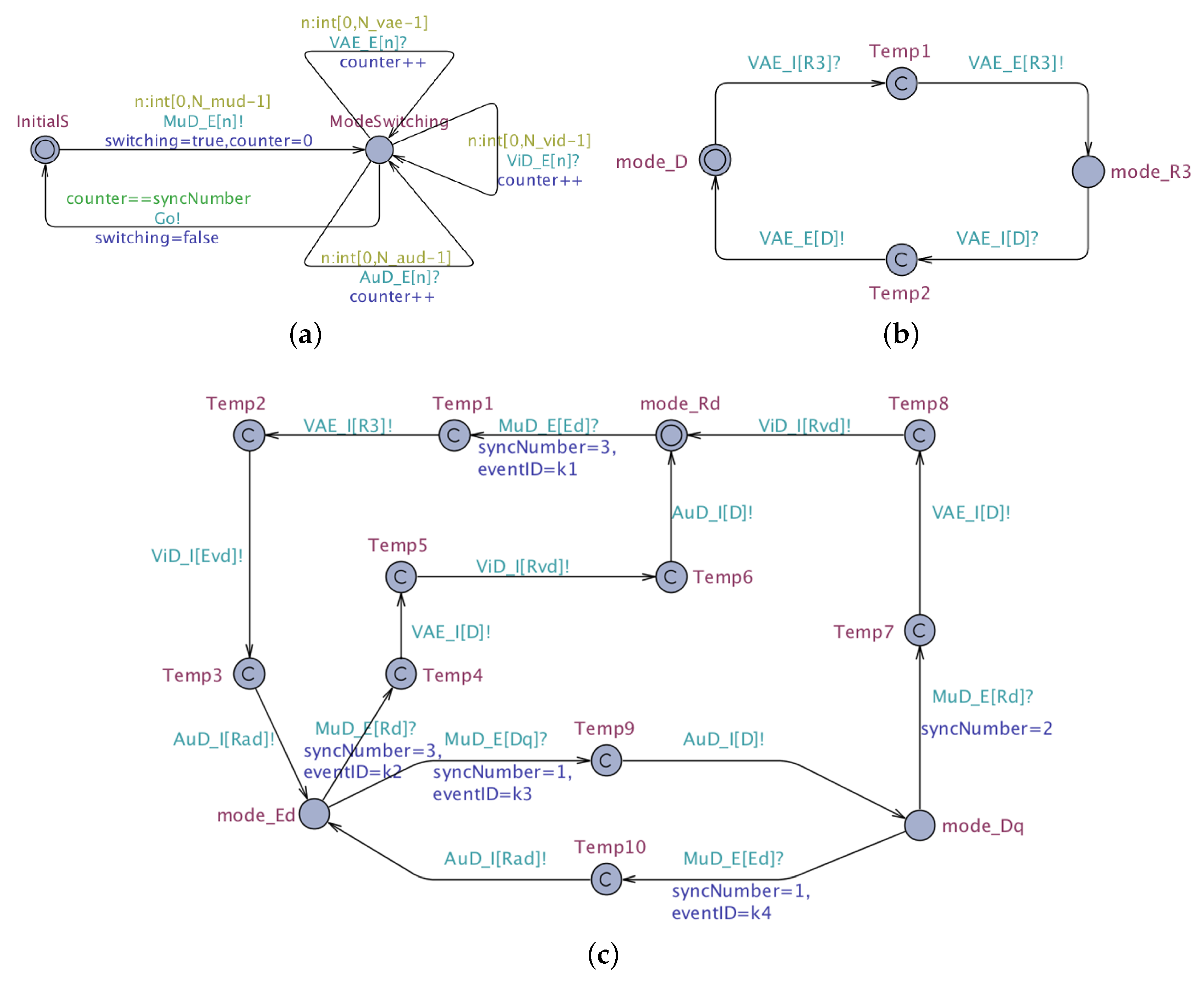
2.4. Mode Mapping Verification

A crucial issue in designing mode mapping with MMA is ensuring the correctness of the mode mapping, i.e., for each input external signal from the mode-switch manager, the set of MMA should produce the expected set of external signals as the output back to the mode-switch manager. For instance, failing to synchronize an internal signal will never yield a mode mapping result.

The mode mapping of a composite component specified by MMA can be easily verified by model checking. We use the model checker UPPAAL [11] for mode mapping verification. Since UPPAAL is a convenient tool for modeling and verifying concurrent state transition systems, it is fairly straightforward to graphically model a set of MMA in UPPAAL. Using UPPAAL, we have modeled (the UPPAAL model is available at http://mdh.diva-portal.org/smash/record.jsf?pid=diva2%3A1244506&dswid=1426) the mode mapping of MuD specified by the set of MMA in Figure 4 and Figure 5.

The behaviors of the local mode-switch manager of MuD, the self-MMA of MuD and the child MMA of its subcomponents are modeled as separate automata in UPPAAL. For instance, Figure 7 showcases three typical UPPAAL models for the mode-switch manager of MuD, ${MMA}_{\mathit{VAE}}^c$ and ${MMA}_{\mathit{MuD}}^s$. Each mode of a component is represented by a state in these UPPAAL models (e.g., mode_R3 represents mode R3 in Figure 7b). These models also contain committed states marked with “C” in a circle, which are intermediate states during a mode-switch. External and internal signals are simulated as channels synchronized between multiple UPPAAL models. For example, VAE_I[R3]! denotes the internal signal VAE.I(R3) emitted by ${MMA}_{\mathit{MuD}}^s$, while VAE_I[R3]? denotes the same signal VAE.I(R3)received by ${MMA}_{\mathit{VAE}}^c$. The UPPAAL model of ${MMA}_{\mathit{MuD}}^s$ in Figure 7c is consistent with ${MMA}_{\mathit{MuD}}^s$ in Figure 4. The reason why the UPPAAL model contains one or more intermediate states for each mode-switch is that receiving and sending each signal needs to be modeled sequentially in UPPAAL. This essentially does not change the execution semantics, as all intermediate states are committed states, whose incoming and outgoing transitions are performed as a single atomic transaction. In addition, shown in Figure 7a, the mode-switch manager of MuD consists of two states. InitialS is the initial state, where the mode-switch manager can send an external signal to ${MMA}_{\mathit{MuD}}^s$ and switch to the state ModeSwitching. Meanwhile, a Boolean variable switching is set to true, indicating an ongoing mode-switch. Depending on the current mode of MuD and the new mode indicated by the external signal from the mode-switch manager, there are four possible events, leading to different transitions among these components: (1) $k_1$: MuD requests to switch from Rd to Ed; (2) $k_2$: MuD requests to switch from Ed to Rd; (3) $k_3$: MuD requests to switch from Ed to Dq; (4) $k_4$: MuD requests to switch from Dq to Ed. Each event ID is assigned to a variable eventID as shown in Figure 7c.

Based on the UPPAAL models, we can verify that the set of MMA of MuD satisfies the expected constraints by checking properties formulated in the UPPAAL query language, which is a subset of timed computation tree logic [12]. The following are four types of properties addressing different constraints:

P1.

A[] not deadlock: The complete set of UPPAAL models is deadlock-free. This is not directly related to mode mapping, but it is a fundamental property that we expect the model to satisfy.

P2.

E$<>$ sMMA_MuD.mode_Ed: It is possible for MuD to run in mode Ed. This property should be verified for all the modes of MuD and its subcomponents.

P3.

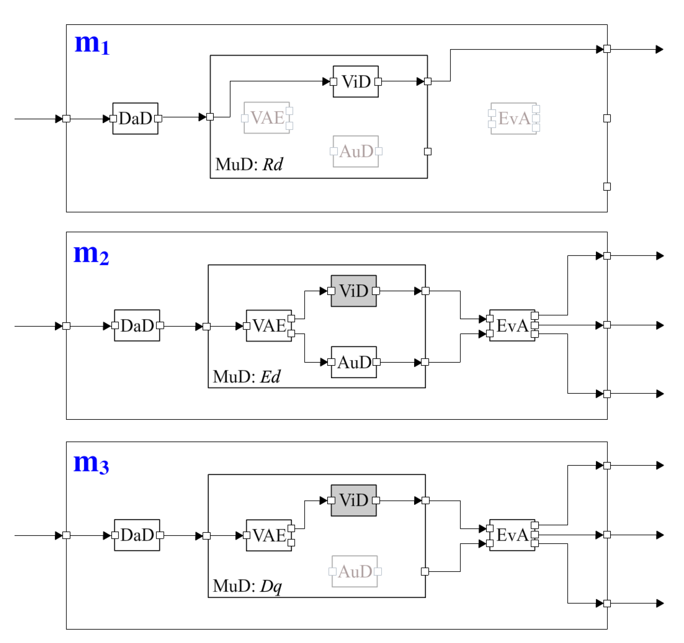
A[] (sMMA_MuD.mode_Rd and !ModeSwitchManager.switching) imply (cMMA_VAE.mode_D and cMMA_ViD.mode_Rvd and cMMA_AuD.mode_D): When MuD runs in Rd, its subcomponents VAE and AuD must be deactivated, while the other subcomponent ViD must run in Rvd. This property should be verified for all possible mode combinations between MuD and its subcomponents according to the mode mapping table in Table 1.

P4.

(ModeSwitchManager.switching and eventID==k1)–>(sMMA_MuD.mode_Ed and cMMA_VAE.mode_R3 and cMMA_ViD.mode_Evd and cMMA_AuD.mode_Rad): An external signal requesting MuD to switch from Rd to Ed will make VAE, ViD and AuD switch to R3, Evd and Rad, respectively. This property should be verified for all possible events from $k_1$–$k_4$.

All these properties are satisfied with verification time less than 4 ms. Furthermore, our UPPAAL models can be used as a common template for modeling any other mode mapping specified by MMA. Due to the graphical resemblance between an MMA and the corresponding UPPAAL model, it is possible to generate UPPAAL models from MMA described by a graphical or textual domain-specific language.

3. Mode Transformation

Our previous research results [9] show that the mode-switch of a multi-mode component may lead to mode-switches of other multi-mode components in the same system, and it is not trivial to coordinate the mode-switches of different components at run-time. The local mode-switch manager of each component needs to run delicate algorithms to communicate with the parent and subcomponents of the component via dedicated mode-switch ports to switch mode cooperatively. Such inter-component communication incurs run-time computation overhead and mode-switch latency. For instance, when MoS in the healthcare monitoring system triggers a mode-switch from Rm to Att, the mode-switch event is first propagated from MoS to MuD and EvA, and MuD subsequently propagates the mode-switch event to VAE, ViD and AuD. Further, more handshake messages are exchanged between these components to keep mode consistency. The communication overhead grows as the component hierarchy becomes more complex.

The purpose of mode transformation is to eliminate the need for the mode-switch coordination among different multi-mode components by a centralized mode management, and thereby achieve better run-time performance, provided that (1) all components are deployed on the same hardware platform and (2) the mode information of each component is globally accessible. Illustrated in Figure 8, mode transformation transfers the responsibility of mode-switch handling from the local mode-switch manager of each component to a single global mode-switch manager. As a result of mode transformation, each multi-mode component becomes unaware of modes. Instead, a global mode transition graph is generated for the global mode-switch manager to handle mode-switch at the system level.

Our mode transformation process includes two sequential steps. First, given the mode mappings of all composite components, we construct an intermediate representation, a mode combination tree (MCT), where all the possible system modes are identified. In the second step, based on a list of possible mode-switch events defined in the system, we add transitions between the identified system modes to construct the mode transition graph. The two steps are further explained in the following subsections separately.

3.1. Construction of the Mode Combination Tree

The aim of constructing the MCT is to identify all the system modes. Let ${\mathcal{M}}_c$ denote the set of supported modes of a component c and D denote the current mode of a deactivated component. Then, we define system modes as follows:

Definition 2.

System modes based on component modes: For a system composed by a set of components $\mathcal{C}=\{c_1,c_2,\cdots ,c_n\}(n\in \mathbb{N})$, the set of system modes is defined as ${\mathcal{M}}_s\subseteq \underset{i\in [1,n]}{\times }\{{\mathcal{M}}_{c_i}\cup \{D\}\}$. Each system mode $m\in {\mathcal{M}}_s$ is a mode combination of all components.

By Definition 2, each system mode $m=(m_{c_1},m_{c_2},\cdots ,m_{c_n})$, where $m_{c_i}\in {\mathcal{M}}_{c_i}\cup \{D\}$ for $i\in [1,n]$. In order to indicate more explicitly the relationship between $c_i$ and $m_{c_i}$, we shall hereafter use an alternative expression to represent a system mode: $m=\{(c_i,m_{c_i})|i\in [1,n]\}$, where $m_{c_i}\in {\mathcal{M}}_{c_i}\cup \{D\}$. Using the same formalism, an MCT is defined as follows:

Definition 3.

Mode combination tree: An MCT is a tree with a set of nodes $\mathcal{N}=\{{\mathcal{N}}_0,{\mathcal{N}}_1,\cdots ,{\mathcal{N}}_n\}(n\in \mathbb{N})$, where ${\mathcal{N}}_0=⌀$ is the root node, and each other node ${\mathcal{N}}_i=\{(c_j,m_{c_j})|j\in [1,k],k\in \mathbb{N}\}(i\in [1,n])$, where for all j, $m_{c_j}\in {\mathcal{M}}_{c_j}\cup \{D\}$ and all $c_j$ have the same depth level in the system component hierarchy.

By Definition 3, each non-root node of an MCT provides a mode combination of components with the same depth level. A typical outlook of MCT is displayed in Figure 9, while the construction of the MCT will be further explained later.

A few more notations and concepts need to be introduced before the formal description of the MCT construction process. First, we introduce the valid local mode combination (LMC) of a composite component c, which is a feasible combination of a mode of c and the modes of all its subcomponents as per the local mode mapping of c. To define the valid LMC of a composite component formally, let $\mathcal{PC}$ and $\mathcal{CC}$ be the set of primitive components and composite components in a system, respectively. Let $\mathit{Top}$ be the component at the top of the component hierarchy in a system. For each $c\in \mathcal{CC}$, a valid LMC of c is formally defined as follows:

Definition 4.

Valid local mode combination: For $c\in \mathcal{CC}$ with ${\mathcal{SC}}_c=\{c_i^1,\cdots ,c_i^n\}$ ($n\in \mathbb{N}$), we call the set ${\mathcal{V}}_c=\{(c,m_c),(c_i^1,m_{c_i^1}),\cdots ,(c_i^n,m_{c_i^n})\}$ a valid LMC of c, where $m_c\in {\mathcal{M}}_c\cup \{D\}$ and $\forall k\in [1,n]$, $m_{c_i}^k\in {\mathcal{M}}_{c_i^k}\cup \{D\}$, if $(m_c,m_{c_i^1},\cdots ,m_{c_i^n})$ is a state of the composed MMA of c.

Note that each element in ${\mathcal{V}}_c$ is a pair $(x,y)$, where $x\in {\mathcal{SC}}_c\cup \{c\}$ and $y\in {\mathcal{M}}_x\cup \{D\}$. For instance, the mode mapping of MoS in Table 1 (a) implies three valid LMCs of MoS: (1) $\{(\mathrm{MoS},Rm),(\mathrm{DaD},R1),(\mathrm{MuD},Rd),(\mathrm{EvA},D)\}$; (2) $\{(\mathrm{MoS},Att),(\mathrm{DaD},R1),(\mathrm{MuD},Ed),(\mathrm{EvA},R2)\}$; (3) $\{(\mathrm{MoS},Att),(\mathrm{DaD},R1),(\mathrm{MuD},Dq),(\mathrm{EvA},R2)\}$.

Based on Definition 4, we further introduce the valid LMC concerning a specific mode of a composite component c, which is a feasible combination of the modes of all subcomponents of c as per the local mode mapping of c when c is running in a particular mode. A formal definition is given as follows:

Definition 5.

Valid LMC concerning a specific mode: For $c\in \mathcal{CC}$ with ${\mathcal{SC}}_c=\{c_i^1,\cdots ,c_i^n\}$ ($n\in \mathbb{N}$), if when c is running in $m_c$, and $\forall c_i^k\in {\mathcal{SC}}_c(k\in [1,n])$, $\exists m_{c_i^k}$ such that $\{(c,m_c),(c_i^1,m_{c_i^1}),\cdots ,(c_i^n,m_{c_i^n})\}$ is a valid LMC of c, then the set ${\mathcal{V}}_{c,m_c}=\{(c_i^1,m_{c_i^1}),\cdots ,(c_i^n,m_{c_i^n})\}$ is a valid LMC of c for $m_c$.

Depending on the mode mapping of c, multiple valid LMCs of c may exist for $m_c$. Let ${\mathcal{W}}_{c,m_c}$ be the set of all valid LMCs of $c\in \mathcal{CC}$ for $m_c$. Each element in ${\mathcal{W}}_{c,m_c}$ is a set ${\mathcal{V}}_{c,m_c}$. The total number of all valid LMCs of c for $m_c$ is $|{\mathcal{W}}_{c,m_c}|$. For instance, according to Table 1 (a), ${\mathcal{W}}_{\mathrm{MoS},Att}=\{{\mathcal{V}}_{\mathrm{MoS},Att}^1,{\mathcal{V}}_{\mathrm{MoS},Att}^2\}$, where ${\mathcal{V}}_{\mathrm{MoS},Att}^1=\{(\mathrm{DaD},R1),(\mathrm{MuD},Ed),(\mathrm{EvA},R2)\}$ and ${\mathcal{V}}_{\mathrm{MoS},Att}^2=\{(\mathrm{DaD},R1),(\mathrm{MuD},Dq),(\mathrm{EvA},R2)\}$. By traversing the states of the composed MMA of c containing $m_c$, it is easy to automatically generate ${\mathcal{W}}_{c,m_c}$.

Next, we introduce an important operator for combining different valid LMCs:

Definition 6.

Valid LMC operation: Consider two sets of valid LMCs ${\mathcal{W}}_1=\{{\mathcal{V}}_1,{\mathcal{V}}_2,\cdots ,{\mathcal{V}}_m\}$ and ${\mathcal{W}}_2=\{{\mathcal{V}}_{k+1},{\mathcal{V}}_{k+2},\cdots ,{\mathcal{V}}_{k+n}\}$, where $m,n,k\in \mathbb{N}$ and $k\ge m$. Let ⊕ be an operator such that ${\mathcal{W}}_1\oplus {\mathcal{W}}_2=\{{\mathcal{V}}_i\cup {\mathcal{V}}_{k+j}|i\in [1,m],j\in [1,n]\}$. In addition, for each $l\in \mathbb{N}$, ${\mathcal{W}}_1\oplus {\mathcal{W}}_2\oplus \cdots \oplus {\mathcal{W}}_l$ can be represented as ${\displaystyle \underset{o\in [1,l]}{⨁}}{\mathcal{W}}_o$.

For the sake of clarity, let us clarify the ⊕ operator using a small example. Suppose ${\mathcal{W}}_1=\{{\mathcal{V}}_1,{\mathcal{V}}_2\}$ where ${\mathcal{V}}_1=\{(a,m_a^1),(b,m_b^1)\}$ and ${\mathcal{V}}_2=\{(a,m_a^2),(b,m_b^2)\}$; and ${\mathcal{W}}_2=\{{\mathcal{V}}_3,{\mathcal{V}}_4\}$ where ${\mathcal{V}}_3=\{(c,m_c^1),(d,m_d^1)\}$ and ${\mathcal{V}}_4=\{(c,m_c^2),(d,m_d^2)\}$. Then,

$$\begin{array}{cc}\hfill {\mathcal{W}}_1\oplus {\mathcal{W}}_2=& \{{\mathcal{V}}_1\cup {\mathcal{V}}_3,{\mathcal{V}}_1\cup {\mathcal{V}}_4,{\mathcal{V}}_2\cup {\mathcal{V}}_3,{\mathcal{V}}_2\cup {\mathcal{V}}_4\}\hfill \\ \hfill =& \{\{(a,m_a^1),(b,m_b^1),(c,m_c^1),(d,m_d^1)\},\hfill \\ & \{(a,m_a^1),(b,m_b^1),(c,m_c^2),(d,m_d^2)\},\hfill \\ & \{(a,m_a^2),(b,m_b^2),(c,m_c^1),(d,m_d^1)\},\hfill \\ & \{(a,m_a^2),(b,m_b^2),(c,m_c^2),(d,m_d^2)\}\}\hfill \end{array}$$

Given the mode mappings of all composite components, the MCT of the system can be constructed by creating nodes top-down from the root node. For each node $\mathcal{N}$ of an MCT, let $d_{\mathcal{N}}$ be its depth level and ${\lambda }_{\mathcal{N}}$ be the number of new nodes created from this node. We use ${\mathcal{N}}_i\succ {\mathcal{N}}_j$ to denote that a new node ${\mathcal{N}}_i$ is created from on old node ${\mathcal{N}}_j$. Moreover, let ${\mathcal{M}}_{\mathit{Top}}=\{m_T^1,m_T^2,\cdots ,m_T^{|{\mathcal{M}}_{\mathit{Top}}|}\}$ be the set of supported modes of $\mathit{Top}$. The MCT is constructed by the following steps:

• From ${\mathcal{N}}_0$, create ${\lambda }_{{\mathcal{N}}_0}=\left|{\mathcal{M}}_{\mathit{Top}}\right|$ new nodes, such that for each new node ${\mathcal{N}}_i\succ {\mathcal{N}}_0$, ${\mathcal{N}}_i=\{(\mathit{Top},m_T^i)\}(i\in [1,|{\mathcal{M}}_{\mathit{Top}}\left|\right])$.
• From each ${\mathcal{N}}_i=\{(\mathit{Top},m_T^i)\}(i\in [1,|{\mathcal{M}}_{\mathit{Top}}\left|\right])$, create ${\lambda }_{{\mathcal{N}}_i}=\left|{\mathcal{W}}_{\mathit{Top},m_T^i}\right|$ new nodes, such that for each ${\mathcal{N}}^{\prime }\succ {\mathcal{N}}_i$, ${\mathcal{N}}^{\prime }\in {\mathcal{W}}_{\mathit{Top},m_T^i}$. Moreover, if ${\lambda }_{{\mathcal{N}}_i}>1$, then for each ${\mathcal{N}}^{\prime },{\mathcal{N}}^{″}\succ {\mathcal{N}}_i$, we have ${\mathcal{N}}^{\prime }\ne {\mathcal{N}}^{″}$.
• For each node $\mathcal{N}=\{(c_1,m_{c_1}),(c_2,m_{c_2}),\cdots ,(c_n,m_{c_n})\}(n\in \mathbb{N})$ with $d_{\mathcal{N}}\ge 2$, if $\forall i\in [1,n]$, $c_i\in \mathcal{PC}$, then $\mathcal{N}$ is marked as a leaf node, and no new node is created from $\mathcal{N}$. Otherwise, if $\exists i\in [1,n]$ such that $c_i\in \mathcal{CC}$, then create ${\lambda }_{\mathcal{N}}={\displaystyle \prod _{\begin{array}{c}i\in [1,n],\\ c_i\in \mathcal{CC}\end{array}}}\left|{\mathcal{W}}_{c_i,m_{c_i}}\right|$ new nodes, such that for each ${\mathcal{N}}^{\prime }\succ \mathcal{N}$, ${\mathcal{N}}^{\prime }\in {\displaystyle \underset{\begin{array}{c}i\in [1,n],\\ c_i\in \mathcal{CC}\end{array}}{⨁}}{\mathcal{W}}_{c_i,m_{c_i}}$. Moreover, if ${\lambda }_{\mathcal{N}}>1$, then for each ${\mathcal{N}}^{\prime },{\mathcal{N}}^{″}\succ \mathcal{N}$, we have ${\mathcal{N}}^{\prime }\ne {\mathcal{N}}^{″}$.
• Repeat Step 3 until all branches of the MCT have reached the leaf node.

The MCT construction process is implemented as Algorithm 1, which is a recursive function $constructMCT(\mathcal{N},d_{\mathcal{N}})$ that has two input parameters: $\mathcal{N}$ is the node currently being explored and $d_{\mathcal{N}}$ is the depth level of $\mathcal{N}$. Initially, $\mathcal{N}=⌀$ and $d_{\mathcal{N}}=0$. We assume that $\mathit{Top}$ must have subcomponents. Otherwise, $\mathit{Top}$ itself will be the entire system, and mode transformation will be meaningless. Moreover, for each component c running in mode m, we assume that ${\mathcal{W}}_{c,m}$ is an indexed set such that ${\mathcal{W}}_{c,m}\left[i\right]$ represents the i-th element of ${\mathcal{W}}_{c,m}$.

Algorithm 1$constructMCT(\mathcal{N},d_{\mathcal{N}})$.

1: if$d_{\mathcal{N}}=0$then   2:  ${\lambda }_{\mathcal{N}}:=\left|{\mathcal{M}}_{\mathit{Top}}\right|$;   3:  for $ifrom1to{\lambda }_{\mathcal{N}}$ do   4:   ${\mathcal{N}}_i:=\{(\mathit{Top},m_T^i)\}$;   5:   $constructMCT({\mathcal{N}}_i,1)$;   6:  end for   7: end if   8: if$d_{\mathcal{N}}=1$then   9:  $\{(\mathit{Top},m)\}:=\mathcal{N}$;  10:  $Derive{\mathcal{W}}_{\mathit{Top},m}$;  11:  ${\lambda }_{\mathcal{N}}:=\left|{\mathcal{W}}_{\mathit{Top},m}\right|$;  12:  for $ifrom1to{\lambda }_{\mathcal{N}}$ do  13:   $constructMCT({\mathcal{W}}_{\mathit{Top},m}\left[i\right],2)$;  14:  end for  15: end if  16: if$d_{\mathcal{N}}\ge 2$then  17:  $\{(c_1,m_{c_1}),(c_2,m_{c_2}),\cdots ,(c_n,m_{c_n})\}:=\mathcal{N}$;  18:  if $\forall i\in [1,n]:c_i\in \mathcal{PC}$ then  19:   return;  20:  else  21:   $Derive\mathcal{W}:={\displaystyle \underset{\begin{array}{c}i\in [1,n],c_i\in \mathcal{CC}\end{array}}{⨁}}{\mathcal{W}}_{c_i,m_{c_i}}$;    22:   ${\lambda }_{\mathcal{N}}:={\displaystyle \prod _{\begin{array}{c}i\in [1,n],c_i\in \mathcal{CC}\end{array}}}\left|{\mathcal{W}}_{c_i,m_{c_i}}\right|$;    23:   for $ifrom1to{\lambda }_{\mathcal{N}}$ do  24:    $constructMCT(\mathcal{W}\left[i\right],d_{\mathcal{N}}+1)$;  25:   end for  26:  end if  27: end if

Once the MCT is constructed, the system modes can be derived as the set of paths from the root node to the leaf nodes of the MCT. The total number of system modes is equal to the total number of leaf nodes of the MCT. Among the system modes, the initial system mode can be recognized based on the specification of the initial modes of all components.

As an example, Figure 9 illustrates the MCT of the monitoring subsystem introduced in Section 1. The MCT consists of nine nodes ${\mathcal{N}}_0$–${\mathcal{N}}_8$ with four depth levels. Represented by the respective paths of the MCT, one of the three identified system modes is:

$$\begin{array}{cc}\hfill m_1=& {\mathcal{N}}_0\cup {\mathcal{N}}_1\cup {\mathcal{N}}_3\cup {\mathcal{N}}_6\hfill \\ \hfill =& \{(\mathit{MoS},Rm),(\mathit{DaD},R1),(\mathit{MuD},Rd),(\mathit{EvA},D),(\mathit{VAE},D),(\mathit{ViD},Rvd),(\mathit{AuD},D)\}\hfill \\ \hfill m_2=& {\mathcal{N}}_0\cup {\mathcal{N}}_2\cup {\mathcal{N}}_4\cup {\mathcal{N}}_7\hfill \\ \hfill =& \{(\mathit{MoS},Att),(\mathit{DaD},R1),(\mathit{MuD},Ed),(\mathit{EvA},R2),(\mathit{VAE},R3),(\mathit{ViD},Evd),(\mathit{AuD},Rad)\}\hfill \\ \hfill m_3=& {\mathcal{N}}_0\cup {\mathcal{N}}_2\cup {\mathcal{N}}_5\cup {\mathcal{N}}_8\hfill \\ \hfill =& \{(\mathit{MoS},Att),(\mathit{DaD},R1),(\mathit{MuD},Dq),(\mathit{EvA},R2),(\mathit{VAE},R3),(\mathit{ViD},Evd),(\mathit{AuD},D)\}\hfill \end{array}$$

Assuming that the monitoring subsystem starts with mode Rm, $m_1$ is the initial system mode after mode transformation. Figure 10 shows the configurations of the three system modes based on the component connections in Figure 1.

The complexity of an MCT depends on the structure of the component hierarchy, the number of modes of each component and the mode mappings in the involved components. The worst-case combination of factors, such as the number of components and the number of component modes, may lead to a huge number of system modes, increasing the overhead exponentially. However, in practice, the expected number of system modes should be limited. If mode transformation becomes intractable due to extreme computation overhead, this would imply that the system is too complex to adopt centralized mode management. Then, it may be more suitable to go for distributed mode management without mode transformation, although the run-time overhead for the required message exchange may be substantial if the component hierarchy is deep. Alternatively, a better solution could be partial mode transformation, i.e., performing mode transformation within one or more composite components instead of the entire system. Our mode transformation technique is flexible enough to support partial mode transformation at any component level. Furthermore, we expect noticeably different behaviors in different modes. Depending on the application, it could be more efficient to merge several modes with similar global configurations into a single mode. The criteria for merging system modes are application-dependent and out of the scope of this article. Nevertheless, we believe that it is possible to partially automate the merging of system modes in a later optimization phase by certain application independent merging rules.

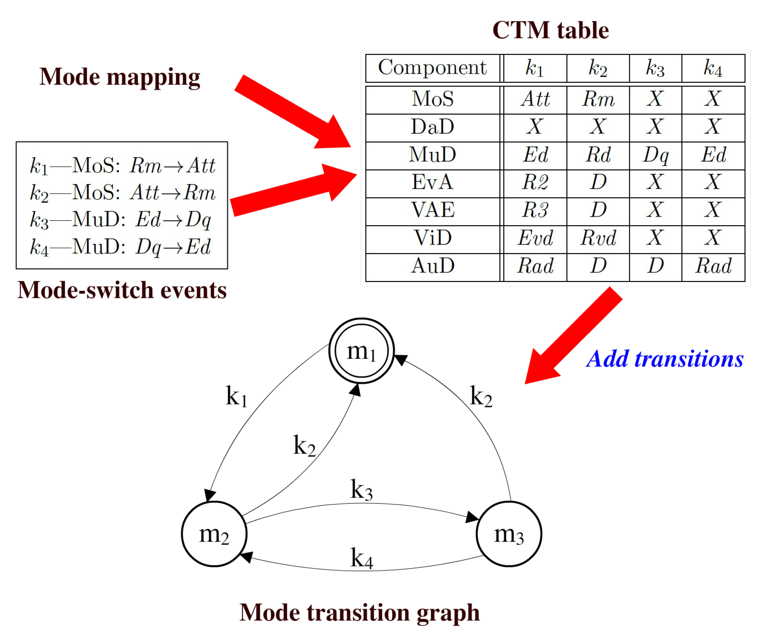
3.2. Deriving the Mode Transition Graph

The constructed MCT identifies system mode, which is subsequently used to derive the mode transition graph on top of these system modes based on the definition of mode-switch events. We assume that a mode-switch event is triggered by a component c requesting to switch mode from $m_c^1$ to $m_c^2$, denoted as $c:m_c^1\to m_c^2$. The triggering of each mode-switch event may lead to the mode-switches of some other components in the same system. For a system with a set of identified system modes $\mathcal{M}=\{m_1,m_2,\cdots ,m_n\}(n\in \mathbb{N})$, a mode-switch is a transition from $m_{old}$ to $m_{new}$, where $m_{old},m_{new}\in \mathcal{M}$ and $m_{old}\ne m_{new}$. A mode transition graph contains all the possible transitions between these system modes and associates each transition with the corresponding mode-switch event. Similar to an MMA, each state of a mode transition graph can be graphically represented by a circle, with the initial state being marked by a double circle. A graphical illustration of the mode transition graph can be found in Figure 11.

The key issue of deriving the mode transition graph is to identify the system modes $m_{old}$ and $m_{new}$ for each mode-switch event for which a system mode-switch is possible. Consider a mode-switch event k identified as $c:m_c^1\to m_c^2$. The only condition satisfying the triggering of k is that the triggering source c is currently running in mode $m_c^1$. For each k, $m_{old}$ can be easily identified as long as $(c,m_c^1)\in m_{old}$. Note that more than one system mode could be identified as $m_{old}$. Depending on the current system mode, a mode-switch event may enable different transitions.

In contrast to $m_{old}$, only one system mode can be the $m_{new}$ for each mode-switch event k. The identification of $m_{new}$ for k is more difficult because it depends not only on $m_c^2$, but also on the target modes of the other components. We identify the $m_{new}$ for each mode-switch event with the assistance of a component target mode (CTM) table. A CTM table is a table with $n_1$ rows and $n_2$ columns, where $n_1$ is the number of components of a system and $n_2$ is the number of mode-switch events. An example of a CTM table is shown above the mode transition graph in Figure 11. In the CTM table, each row is associated with a component, each column is associated with a mode-switch event and each cell contains the target mode $m_c$ of the corresponding component c for the corresponding mode-switch event k. The cell with X indicates that $m_c$ is independent of k, i.e., k does not lead to the mode-switch of c.

A CTM table can be automatically constructed offline based on the list of mode-switch events and the mode mapping of each composite component. Let $m_c^k$ be the target mode of c for k in a CTM table. Taking advantage of the CTM table, the new system mode $m_{new}$ for each mode-switch event k can be identified as follows: For each system mode $m=\{(c_i,m_{c_i})|i\in [1,n],n\in \mathbb{N}\}$, if $\forall i$ where $m_{c_i}^k\ne X$ in the CTM table (i.e., k leads to the mode-switch of $c_i$ to a new mode $m_{c_i}^k$), we have $m_{c_i}=m_{c_i}^k$, then m is the $m_{new}$ for k. Algorithm 2 describes the process of building the mode transition graph, with a search space of $O(|\mathcal{M}|·|\mathcal{K}|)$.

Algorithm 2$constructMTG(\mathcal{C},\mathcal{M},\mathcal{K})$.

1: $\mathcal{C}=\{c_1,\cdots ,c_o\}(o\in \mathbb{N})$; {$The set of all components$}   2: $\mathcal{M}=\{m_1,\cdots ,m_n\}(n\in \mathbb{N})$; {$The set of identified system modes$}   3: $\mathcal{K}=\{k_1,\cdots ,k_l\}(l\in \mathbb{N})$; {$The set of all mode-switch events$}   4: for all$k_i\in \mathcal{K}wherek\in [1,l]and{k}_i=c:m_c^1\to m_c^2$do   5:  if $\exists m_j\in \mathcal{M}s.t.(\forall c_p\in \mathcal{C}and{m}_{c_i}^{k_i}\ne X,(c_p,m_{c_p}^{k_i})\in m_j)$ then   6:   $m_{new}=m_j$;   7:   for all $m_j\in \mathcal{M}$ do   8:    if $(c,m_c^1)\in m_j$ then   9:     $addTransition(m_j,m_{new},k_i)$; {$Add a transition from{m}_{j}to{m}_{new}labeled with{k}_i$}  10:    end if  11:   end for  12:  end if  13: end for

Figure 11 presents the workflow for deriving the mode transition graph of the monitoring subsystem. The CTM table is derived based on two inputs: (1) the mode mapping of composite components MoS and MuD specified by MMA and (2) the possible mode-switch events. For this example, four mode-switch events, from $k_1$–$k_4$, are specified at design time. $k_1$ and $k_2$ are triggered by MoS for switching between modes Rm and Att, while $k_3$ and $k_4$ are triggered by MuD for switching between modes Ed and Dq. The target modes of all components in the monitoring subsystem for all mode-switch events are listed in the CTM table. Previously, the MCT in Figure 9 has identified three system modes $m_1$ (the initial mode), $m_2$ and $m_3$. The CTM table additionally adds transitions between the system modes based on each possible mode-switch event, thereby yielding the mode transition graph. The mode transition graph helps the global mode-switch manager to keep track of the current system mode and makes the system switch to the right target mode when a mode-switch is triggered.

After mode transformation, local mode-switch managers are replaced with a single global mode-switch manager, whose complexity is much lower than each local mode-switch manager. A local mode-switch manager needs complex algorithms [9] to coordinate mode-switches between a composite component and its subcomponents, such as checking component states before mode-switch is performed, handling multiple concurrent mode-switch events triggered by different components and handling emergency mode-switch events, which are more critical than regular mode-switch events. By contrast, the global mode-switch manager only takes care of system mode based on a single CTM table.

Mode transformation assumes no dynamic change of modes or mode mappings at any level. If there is a need to change the mode of a component or its mode mapping (e.g., adding new modes, removing modes, changing mode names), then mode transformation must be applied again from scratch. The chain effect of such a change must be considered when it is propagated to other components. The change of mode mapping of one component may entail the change of mode mapping of its parent component and subcomponents. The architecture designer should decide how to update the MMA of components impacted by a change. Mode transformation can always be automated in the same way once all MMA are in place.

A potential drawback of mode transformation is the loss of potential concurrency between local mode managers. If multiple mode-switch events are triggered concurrently and affect disjoint sets of components, distributed mode management before mode transformation allows that these mode-switch events can be handled concurrently, whereas different mode-switch events have to be sequentially handled by the global mode-switch manager. Nonetheless, the centralized mode management after mode transformation eliminates inter-component communication, which is a complex process [9]. Hence, mode transformation is still more likely to yield a faster mode-switch.

The correctness of the two steps of mode transformation has been verified by manual theorem proving. All the detailed theorems and proofs can be found in the extended technical report [10].

3.3. Concrete Implementation of Mode Transformation

A prototype tool MCORE [13], the Multi-mode COmponent Reuse Environment, has been developed to support the modeling of multi-mode systems with multi-mode components by integrating mode mapping and mode transformation. Compared with other component-based development tools, a distinguishing feature of MCORE is the reuse of multi-mode software components. As far as we know, MCORE is the first (and possibly only) tool for building multi-mode systems with multi-mode components. MCORE can be potentially used as a preprocessor for Rubus ICE [14], which is an IDEfor the Rubus component model [15] developed by Arcticus Systems (http://www.arcticus-systems.com/). As an industrial component model, Rubus is targeting the component-based development of vehicular systems. Rubus supports multi-mode systems; however, modes can only be specified at the system level, and the reuse of multi-mode components is not supported. This limitation can be alleviated by MCORE. The system model built by multi-mode components in MCORE is in compliance with the Rubus component model after mode transformation. Hence, the system model designed in MCORE can be imported to Rubus ICE for further analysis, test and code generation.

4. Related Work

The extended MECHATRONICUML [16,17] (EUML) allows the hierarchical composition of reconfigurable components, which are comparable to our multi-mode components. EUML introduces an additional reconfiguration port for each component, which resembles the dedicated mode-switch ports of a multi-mode component. In EUML, the reconfiguration of a composite component is handled by two dedicated subcomponents, which play similar roles as the local mode-switch manager of a multi-mode component. Unlike our approach, EUML does not pre-define component configurations at design-time, thus allowing more flexible reconfiguration at run-time. Compared with such reconfigurable systems, multi-mode systems built by multi-mode components are more predictable due to static configurations specified at design-time.

Pop et al. proposed an Oracle-based approach [18] that also supports the reuse of multi-mode components. Component behaviors are abstracted into a global property network. Component mode is treated as a property dependent on other property values. The change of one property is propagated throughout the property network, potentially leading to the change of other properties. At the end of propagation, component modes are updated top-down. Similar to our mode transformation, a finite-state machine called Oracle is offline constructed to guarantee a predictable update time of the property network. The mapping between component modes is however not systematically specified in the Oracle-based approach.

Weimer et al. proposed a set of input-output blocks for building multi-mode systems [19]. Each multi-mode component contains a set of mode blocks (MBs), while each MB includes all the components used for the corresponding mode. The mode-switch of a component is achieved by switching the currently selected MB controlled by a supervisor block (SB). These blocks were implemented in Simulink [20]. Another work similar to this is the mode-oriented design [21] in Gaspard2 [22]. A multi-mode component is represented by a macro component, which consists of a state graph component and one or more mode-switch components. A mode-switch component plays the same role as the MB in [19]. Both approaches in [19,21] use completely different components for different modes, whereas in our approach, it is possible to share some components and connections in different modes. Hence, our approach is more suitable for the reuse of multi-mode components.

Mode-switch has been addressed in a number of component models, e.g., SaveCCM [23], COMDES-II [24] and MyCCM-HI [25], to name a few. There are also some other component models that have been commercialized, e.g., Koala [26] (targeting consumer electronics) and Rubus [15] (targeting ground vehicles). These component models have different notions of mode-switch handling. Koala and SaveCCM both use a special connector switch to achieve the structural diversity of a component. switch selects outgoing connections based on input data. In COMDES-II, a state-machine component switches component configurations in different modes. Rubus only considers system-level mode, which is in line with our system mode after mode transformation. MyCCM-HI supports mode-aware components whose mode-switch is controlled by a mode automaton associated with each component. Another component model supporting component reconfiguration is Fractal [27]. Each Fractal component has a membrane (a container for local controllers) that is able to control the reconfiguration of the component.

Mode-switch has also been covered by some programming and specification languages, such as AADL [28], Giotto [29], TDL [30], the extended Darwin [31] and mode-automata [32]. In AADL, component mode-switch is represented by a state machine, including states, transitions and input/output event ports used for mode-switch triggering. Both Giotto and TDL are time-triggered languages for embedded programming, which require periodic checking of conditions to decide whether to trigger a mode-switch or not. The extended Darwin [31] extends the existing Architecture Description Language Darwin [33] by incorporating the notion of mode. The mode of a composite component is directly related to the modes of its subcomponents. Yet, the mapping between modes is unclear in [31]. Mode-automata is a programming model supporting the description of running modes of reactive systems. The behavior of a system is a sequence of modes, each of which corresponds to a collection of execution states. Our MMA differs from mode-automata in the sense that mode-automata specifies the hierarchical structure of system-wide modes, whereas MMA specifies the local mode mapping within composite components.

Dynamic software product lines (DSPL) [34], which originates from the conventional software product lines (SPL) [35] for producing a family of software systems, is an emerging technique for developing adaptive systems. Different systems configured from the same SPL share certain common features, whereas the SPL uses variation points to distinguish the unique features of each system. DSPL allows the binding of variation points at run-time so that a system can dynamically change configurations on the fly to accommodate the changing environment. DSPL is becoming more adaptive [36]; however, to the best of our knowledge, DSPL only considers global system configurations without considering reuse of adaptive software components.

Different types of automata have been proposed for component-based systems and multi-mode systems. For instance, constraint automata [37] is used to model the functional coordination of components, thereby enabling the formal verification of coordination mechanisms. Besides, multi-mode automata [38] is intended for compositional analysis of multi-mode real-time systems. The MMA presented in this article serves as a formalism for a unique and dedicated purpose: mode mapping, which to our knowledge has not been addressed by other existing automata.

Criado et al. [39] proposed a method for an adaptive component-based architecture using model transformation. Software architecture can be dynamically constructed based on transformation rules defined in a repository. Their proposal was applied to component-based GUIs for web applications. Compared to our approach, their adaptation runs at the system level only.

5. Conclusions and Future Work

Partitioning system behaviors into modes and component-based software engineering are both successful software development methods to tame the growing software complexity of modern cyber-physical systems (CPS). It is still an under-researched area to combine both methods, due to their conflicting natures: multi-mode systems are built top-down, while component-based systems are built bottom-up. In this article, we combine the advantages of both methods and propose the component-based software development of multi-mode systems, characterized by the reuse of multi-mode components, i.e., components that can run in different modes and switch mode guided by a local mode-switch manager. We specify the local mode mapping of each composite component by mode mapping automata. Mode mapping is then complemented by a mode transformation technique that transforms component modes to system modes for centralized mode management to improve the mode-switch performance, since the transformation eliminates the need for inter-component communication to coordinate a mode-switch at run-time, thereby reducing mode-switch overhead and shortening mode-switch time. Mode transformation is an optional and flexible process that can be taken for the entire system if the mode information of all components is globally accessible and all software components are deployed on the same hardware platform, or within certain composite components instead of the entire system. It can even be performed iteratively. For instance, in scenarios where systems are built from composite components provided by different vendors that do not want to reveal the internal structure of their components to the integrator, each vendor could apply mode transformation on the level of their respective composite component, and the integrator could then compose the resulting mode-mappings to a system-wide centralized mode management.

The healthcare monitoring system introduced in this article is only a proof-of-concept guiding example. In future work, our software development approach should be further evaluated, and before being deployed, its applicability and concrete implementation should be explored in more substantial real-world systems. Moreover, some remaining efforts need to be invested to complete the development of our prototype tool MCORE fully and its integration in the commercial tool Rubus ICE developed by Arcticus Systems. This will allow us to develop reusable multi-mode software components in MCORE as a preprocessor of Rubus ICE, perform mode transformation therein and then export the system model with global system modes to Rubus ICE for further analysis, test and code generation. Still, the actual effects in terms of resulting improvements, additional and/or reduced efforts, improved quality, etc., throughout the life-cycle of a CPS require empirical evidence much beyond what is presented in this article.

At a more general level, this article presents essential bricks and related glue for a small part of the wall needed to tame the complexity of CPS-related development and life-cycle challenges to a level that allows future deployment of the many technical solutions required to address several of the key challenges of modern society successfully. Many more bricks are however needed, as well as the glue that enables their successful composition.

References

1. Rajkumar, R.; Lee, I.; Sha, L.; Stankovic, J. Cyber-physical systems: The next computing revolution. In Proceedings of the Design Automation Conference, Anaheim, CA, USA, 13–18 June 2010; pp. 731–736. [Google Scholar]
2. Degani, A.; Kirlik, A. Modes in human-automation interaction: Initial observations about a modeling approach. In Proceedings of the IEEE International Conference on Systems, Man, and Cybernetics, Vancover, BC, Canada, 22–25 October 1995; pp. 3443–3450. [Google Scholar]
3. Crnković, I.; Larsson, M. Building Reliable Component-Based Software Systems; Artech House: Norwood, MA, USA, 2002. [Google Scholar]
4. Crnković, I.; Sentilles, S.; Vulgarakis, A.; Chaudron, M.R.V. A Classification Framework for Software Component Models. IEEE Trans. Softw. Eng. 2011, 37, 593–615. [Google Scholar] [CrossRef]
5. Pop, T.; Hnětynka, P.; Hošek, P.; Malohlava, M.; Bureš, T. Comparison of component frameworks for real-time embedded systems. Knowl. Inf. Syst. 2013, 1–44. [Google Scholar] [CrossRef]
6. Yin, H.; Hansson, H. A mode mapping mechanism for component-based multi-mode systems. In Proceedings of the 4th Workshop on Compositional Theory and Technology for Real-Time Embedded Systems, Vienna, Austria, 29 November–2 December 2011; pp. 38–45. [Google Scholar]
7. Yin, H.; Hansson, H. Flexible and efficient reuse of multi-mode components for building multi-mode systems. In Proceedings of the 14th International Conference on Software Reuse, Miami, FL, USA, 4–6 January 2015; pp. 237–252. [Google Scholar]
8. Yin, H.; Hansson, H. Handling multiple mode-switch scenarios in component-based multi-mode systems. In Proceedings of the 20th Asia-Pacific Software Engineering Conference, Ratchathewi, Bangkok, Thailand, 2–5 December 2013; pp. 404–413. [Google Scholar]
9. Yin, H.; Hansson, H. Handling emergency mode-switch for component-based systems. In Proceedings of the 21st Asia-Pacific Software Engineering Conference, Jeju, Korea, 1–4 December 2014; pp. 158–165. [Google Scholar]
10. Yin, H.; Hansson, H.; Orlando, D.; Miscia, F.; Marco, S.D. Component-Based Software Development of Multi-Mode Systems—An Extended Report; Technical Report MDH-MRTC-312/2016-1-SE; Mälardalen University: Västerås, Sweden, 2016. [Google Scholar]
11. Larsen, K.G.; Pettersson, P.; Yi, W. UPPAAL in a nutshell. Int. J. Softw. Tools Technol. Transf. 1997, 1, 134–152. [Google Scholar] [CrossRef]
12. Alur, R.; Courcoubetis, C.; Dill, D. Model-checking for real-time systems. In Proceedings of the 5th Annual IEEE Symposium on Logic in Computer Science, Philadelphia, PA, USA, 4–7 June 1990; pp. 414–425. [Google Scholar]
13. Miscia, F. Design and Implementation of the MCORE IDE: A Multi-Mode COmponent Reuse Environment. Master’s Thesis, University of L’Aquila, L’Aquila, Italy, 2015. [Google Scholar]
14. Systems, A. Rubus ICE. Available online: https://www.arcticus-systems.com/products/ (accessed on 20 October 2018).
15. Hänninen, K.; Mäki-Turja, J.; Nolin, M.; Lindberg, M.; Lundbäck, J.; Lundbäck, K. The Rubus component model for resource constrained real-time systems. In Proceedings of the 3rd International Symposium on Industrial Embedded Systems, La Grande Motte, France, 11–13 June 2008; pp. 177–183. [Google Scholar]
16. Schubert, D.; Heinzemann, C.; Gerking, C. Towards Safe Execution of Reconfigurations in Cyber-Physical Systems. In Proceedings of the 2016 19th International ACM SIGSOFT Symposium on Component-Based Software Engineering (CBSE), Venice, Italy, 5–8 April 2016; pp. 33–38. [Google Scholar]
17. Heinzemann, C.; Becker, S.; Volk, A. Transactional Execution of Hierarchical Reconfigurations in Cyber-Physical Systems. Softw. Syst. Model. 2017. [Google Scholar] [CrossRef]
18. Pop, T.; Plasil, F.; Outly, M.; Malohlava, M.; Bures, T. Property networks allowing oracle-based mode-change propagation in hierarchical components. In Proceedings of the 15th International ACM SIGSOFT Symposium on Component Based Software Engineering, Bertinoro, Italy, 25–28 June 2012; pp. 93–102. [Google Scholar]
19. Weimer, J.E.; Krogh, B.H. Hierarchical Modeling of Mode-Switching Systems. In Proceedings of the 2007 Summer Computer Simulation Conference, San Diego, CA, USA, 15–18 July 2007; pp. 567–574. [Google Scholar]
20. MathWorks. Simulink. Available online: http://se.mathworks.com/products/simulink/ (accessed on 20 October 2018).
21. Quadri, I.R.; Gamatié, A.; Boulet, P.; Dekeyser, J.L. Modeling of Configurations for Embedded System Implementations in MARTE. In Proceedings of the 1st Workshop on Model Based Engineering for Embedded Systems Design, Dresden, Germany, 12 March 2010. [Google Scholar]
22. Gamatié, A.; Beux, S.L.; Piel, E.; Etien, A.; Atitallah, R.B.; Marquet, P.; Dekeyser, J.L. A Model Driven Design Framework for High Performance Embedded Systems; Technical Report RR-6614; Institut National de Recherche en Informatique et Automatique: Rocquencourt, France, 2008. [Google Scholar]
23. Hansson, H.; Åkerholm, M.; Crnković, I.; Törngren, M. SaveCCM—A component model for safety-critical real-time systems. In Proceedings of the Euromicro Conference, Special Session on Component Models for Dependable Systems, Rennes, France, 31 August–3 September 2004; pp. 627–635. [Google Scholar]
24. Ke, X.; Sierszecki, K.; Angelov, C. COMDES-II: A Component-Based Framework for Generative Development of Distributed Real-Time Control Systems. In Proceedings of the 13th IEEE International Conference on Embedded and Real-Time Computing Systems and Applications, Daegu, Korea, 21–24 August 2007; pp. 199–208. [Google Scholar]
25. Borde, E.; Haïk, G.; Pautet, L. Mode-based reconfiguration of critical software component architectures. In Proceedings of the Conference on Design, Automation and Test in Europe, Nice, France, 20–24 April 2009; pp. 1160–1165. [Google Scholar]
26. Ommering, R.V.; Linden, F.V.D.; Kramer, J.; Magee, J. The Koala component model for consumer electronics software. Computer 2000, 33, 78–85. [Google Scholar] [CrossRef] [Green Version]
27. Bennour, B.; Henrio, L.; Rivera, M. A reconfiguration framework for distributed components. In Proceedings of the 2009 ESEC/FSE Workshop on Software Integration and Evolution, Amsterdam, The Netherlands, 25 August 2009; pp. 49–56. [Google Scholar]
28. Feiler, P.H.; Gluch, D.P.; Hudak, J.J. The Architecture Analysis & Design Language (AADL): An Introduction; Technical Report CMU/SEI-2006-TN-011; Software Engineering Institute: Pittsburgh, PA, USA, 2006. [Google Scholar]
29. Henzinger, T.A.; Horowitz, B.; Kirsch, C.M. Giotto: A time-triggered language for embedded programming. Proc. IEEE 2003, 91, 84–99. [Google Scholar] [CrossRef]
30. Templ, J. TDL Specification and Report; Technical Report; Department of Computer Science, University of Salzburg: Salzburg, Austria, 2003. [Google Scholar]
31. Hirsch, D.; Kramer, J.; Magee, J.; Uchitel, S. Modes for software architectures. In Proceedings of the 3rd European Conference on Software Architecture, Nantes, France, 4–5 September 2006; pp. 113–126. [Google Scholar]
32. Maraninchi, F.; Rémond, Y. Mode-Automata: About Modes and States for Reactive Systems. In Proceedings of the European Symposium on Programming, Lisbon, Portugal, 28 March–4 April 998; pp. 185–199.
33. Magee, J.; Dulay, N.; Eisenbach, S.; Kramer, J. Specifying Distributed Software Architectures. In Proceedings of the 5th European Software Engineering Conference, Sitges, Spain, 25–28 September 1995; pp. 137–153. [Google Scholar]
34. Capilla, R.; Bosch, J.; Trinidad, P.; Ruiz-Cortés, A.; Hinchey, M. An overview of Dynamic Software Product Line architectures and techniques: Observations from research and industry. J. Syst. Softw. 2014, 91, 3–23. [Google Scholar] [CrossRef] [Green Version]
35. Clements, P.; Northrop, L. Software Product Lines: Practices and Patterns; Addison-Wesley: Boston, MA, USA, 2001. [Google Scholar]
36. Sharifloo, A.M.; Metzger, A.; Quinton, C.; Baresi, L.; Pohl, K. Learning and Evolution in Dynamic Software Product Lines. In Proceedings of the 11th International Symposium on Software Engineering for Adaptive and Self-Managing Systems, Austin, TX, USA, 14–22 May 2016; pp. 158–164. [Google Scholar]
37. Baier, C.; Sirjani, M.; Arbab, F.; Rutten, J. Modeling component connectors in Reo by constraint automata. Sci. Comput. Program. 2006, 61, 75–113. [Google Scholar] [CrossRef]
38. Phan, L.T.X.; Lee, I.; Sokolsky, O. Compositional Analysis of Multi-mode Systems. In Proceedings of the 22nd Euromicro Conference on Real-Time Systems, Brussels, Belgium, 6–9 July 2010; pp. 197–206. [Google Scholar]
39. Criado, J.; Rodríguez-Gracia, D.; Iribarne, L.; Padilla, N. Toward the adaptation of component-based architectures by model transformation: Behind smart user interfaces. Softw. Pract. Exp. 2015, 45, 1677–1718. [Google Scholar] [CrossRef]
Figure 1. The architectural model of a multi-mode system built from multi-mode components.
Designs 02 00039 g001
Figure 2. The illustration of a multi-mode component.
Designs 02 00039 g002
Figure 3. The role of the mode mapping of MuD at run-time. MMA, mode mapping automata.
Designs 02 00039 g003
Figure 4. The self-mode mapping automaton of MuD.
Designs 02 00039 g004
Figure 5. The child mode mapping automata of MuD.
Designs 02 00039 g005
Figure 6. MMA composition for MuD.
Designs 02 00039 g006
Figure 7. UPPAALmodels of the mode mapping of MuD. (a) UPPAAL model for the mode-switch manager of MuD. (b) UPPAAL model for the child MMA of VAE. (c) UPPAAL model for the self-MMA of MuD.
Designs 02 00039 g007
Figure 8. The overview of mode transformation.
Designs 02 00039 g008
Figure 9. The mode combination tree of the monitoring subsystem.
Designs 02 00039 g009
Figure 10. The configurations of different system modes after mode transformation.
Designs 02 00039 g010
Figure 11. Deriving the mode transition graph of the monitoring subsystem. CTM, component target mode.
Designs 02 00039 g011