Review

Review: Deep Learning-Based Survival Analysis of Omics and Clinicopathological Data

Bioinformatics Platform, Centro de Investigación Biomédica en Red Enfermedades Hepáticas y Digestivas (CIBEREHD), Instituto de Salud Carlos III, Monforte de Lemos 3-5, Pabellón nº 11, 8029 Madrid, Spain
*
Author to whom correspondence should be addressed.
Inventions 2024, 9(3), 59; https://doi.org/10.3390/inventions9030059
Submission received: 30 March 2024 / Revised: 4 May 2024 / Accepted: 11 May 2024 / Published: 16 May 2024

Abstract

:
The 2017–2024 period has been prolific in the area of the algorithms for deep-based survival analysis. We have searched the answers to the following three questions. (1) Is there a new “gold standard” already in clinical data analysis? (2) Does the DL component lead to a notably improved performance? (3) Are there tangible benefits of deep-based survival that are not directly attainable with non-deep methods? We have analyzed and compared the selected influential algorithms devised for two types of input: clinicopathological (a small set of numeric, binary and categorical) and omics data (numeric and extremely high dimensional with a pronounced p >> n complication).

1. Introduction

The famous Vapnik’s “Statistical learning theory” starts with an argument that for the sake of efficiency, almost every statistical problem can be reformulated as a pattern recognition problem. In the clinical literature, doing so is informally referred to as machine learning (ML). Deep learning (DL) is a leading paradigm in ML, which recently has brought notable improvements in benchmarks and provided principally new functionalities. The shift towards the deep extends the horizons in seemingly every field of clinical bioinformatics, for example, biomarkers have been discovered for the conditions for which there is no statistical counterpart [1].
Similar to a regression problem, in survival analysis, there are covariates describing a patient and a numeric response variable, which represents the time until an event (e.g., death). Yet, there is an important complication of censoring, namely, the true event times are typically unknown for a substantial fraction of patients because the follow-up is not long enough for the event to happen, or the patient leaves the study before its termination—any subject that has not failed by the end of the study is right-censored. This complication makes the usual methods of analysis such as regression or a two-sample test inappropriate. To circumvent this problem, indigenous algorithms were designed, and by 1975, the survival analysis became “the gold standard in medical statistics” [2] with the three main statistical methodologies: (1) the Kaplan–Meier graph for a visual comparison of the probability of survival in group A vs. group B; (2) the log-rank test to confirm whether one group has better survival prospects than the other, and the observed differences are not due to random variability; and (3) the Cox model to carry out a full regression analysis.
As far as DL is concerned, in the context of modern hardware and flexible software frameworks, the research community revisited the idea of Faraggi–Simon [3] to approximate the effect of the covariates h ( x ) directly with a NN. The old failure to outperform the Cox model was explained with the lack of infrastructure and the under-developed theoretical apparatus. A large number of primary research articles on the topic have been published, and an interested reader can be referred to a review by [4] for an exhaustive enumeration of the algorithms up to to the end of 2022 and their systematic characterization in the space of the alternatives of DL. Currently, the motivation for developing neural network-based survival algorithms is broader than that of outperforming the classical survival methods and includes developing a principally new research paradigm for fundamental biological research.
The research questions of this article are as follows.
RQ1: Does the DL component lead to a notably improved performance? Unlike for images, for omics and clinicopathological covariates, a DL-based variant does not necessarily lead to a notably higher value of the success metric as compared to the Cox model.
RQ2: Are there tangible benefits of deep-based survival that are not directly attainable with non-deep methods? There are several DL-specific advantages, including (a) a new type of interpretability, for example, via the architectures constrained with biological knowledge about genes and how they are organized into pathways, (b) biomarkers based on hundreds of weak covariates may potentially be constructed, when no economic biomarker is available, and (c) gaining part of the solution in terms of weights from a connected and already solved problems via transfer learning.
RQ3: Is there a new “gold standard” [2] already for survival analysis with models implementing a neural network in clinical data analysis of omics and clinicopathological data (i.e., whether deep-based survival has substituted the Cox model in mission critical routine analysis)? The critical mass of technical research has been reached, in the sense that the DL-based survival methods have been applied in routine mission critical analysis published in central clinical journals, but statistical analysis as with the Cox glmnet() library in R remains the most used.
It should be added that due to the interdisciplinary nature of the topic, sometimes the answers cannot be directly taken from the primary research articles, as the research objectives and success criteria mismatch across different research fields [5]. For example, in neural network research, the contribution can be a new algorithm that is more accurate than the CoxPH, which is not easy either, and yet clinical bioinformatics poses many more requirements such as interpretability, calibration, clinical utility, etc.
The rest of the article is organized as follows. In Section 2, the Cox model is briefly described. Section 2 provides the rationale for the development of the survival methods with a deep neural network component. Section 3 contains the selected algorithms, a comparison of their performance and mentions the first studies in central clinical journals where these algorithms were used for routine analysis. The completed uniform graphical representation of neural architectures reveals several recyclable traits across different architectures, and these are included in the Discussion in Section 5. Finally, in Section 4, the answers to the research questions are formulated.

2. The Cox Model

For each individual i, there is a true survival time T and a true censoring time C, at which the patient drops out of the study or the study ends, and T i = m i n ( T , C ) . The status indicator is available for every observation:
δ = 1, if the event time is observed, and
δ = 0, if censoring time is observed.
Every data point has a vector X of p features associated to it, also termed as attributes or covariates. The data point corresponding to the individual i can be specified as ( T i , δ i , X i ) . The objective is to predict the true survival time T, while modeling it as a function of covariates. T can be discrete or continuous. The Cox model specifies that the hazard function h ( t | x i ) (also called the force of mortality) has the form of
h ( t | X i ) = h 0 ( t ) e x p ( j = 1 p x i j β j ) ,
where no assumption is made about the functional form of h 0 ( t ) , called the baseline hazard. The part h 0 ( t ) cancels out in the process of the derivation of the partial likelihood of the data, which is maximized with respect to β :
P L ( β ) = i : δ i = 1 e x p ( j = 1 p x i j β j ) i : y i y i e x p ( j = 1 p x i j β j ) .
The hazard is the probability that an individual who is under observation at time t has an event at this time; thus, a greater hazard signifies a greater risk of the event. When X comprises only fixed covariates, the model is referred to as the proportional hazard model. (Cox allows the covariate vector to contain time-dependent elements, in which case the covariate vector is written X ( t ) . The extension to time-dependent covariates is important and leads to models where the hazards are typically nonproportional. In this article, the equations describe the Cox proportional hazard model.) The cause of failure can be singular or from a set of cause-specific competing hazards that are not assumed to be independent (e.g., death from cancer or treatment complications). The diminishing with time probability of surviving is expressed via the decreasing survival function S ( t ) = P r ( T > t ) . There is a clearly defined relationship between S ( t ) and h ( t ) , which is given by the formula:
h ( t ) = d d t [ l o g S ( t ) ] ,
where the point is that if either S ( t ) or h ( t ) is known, the other is automatically determined.
As has been said above, to estimate β , the partial likelihood is maximized with respect to β . Other parameters can be estimated in the same manner: p-values corresponding to a particular null hypotheses, as well as confidence intervals associated with the coefficients. Although Equation (2) is known as a partial likelihood, not likelihood, as it does not correspond exactly to the probability of data under assumption, it is a very good approximation [6].
An interested reader can be referred to a review of 50 years of statistical research related to the Cox model [7] mentioning a current concern that the relative risk is not causal.
As far as DL is concerned, in the context of modern hardware and flexible software frameworks, the research community revisited the idea of Faraggi–Simon [3] to approximate the effects of patient’s covariates on their hazard rate directly with a NN, which looked promising since a potentially limiting assumption of the Cox model would be relaxed; while, as discussed in [8], the model assumes that a patient’s log-rank risk is a linear combination of the covariates, it may be oversimplistic to assume that the log-risk function is linear, and instead, genes (gene expressions are modeled as covariates) can engage in higher-order interactions. Neural networks can handle these non-linear relationships and higher-order interactions among the features. To this end, the j = 1 p x i j β j from Equation (1) can be substituted with a NN that takes X as an input and outputs h ( X ) .
The central success metric in survival analysis is the C-index, which estimates the probability that for a random pair of individuals, the predicted survival times have the same ordering as their true survival times. The C-index approximates the area under the ROC curve (AUC). Typically, high values of C > 0.8 are needed to prove the validity of a new clinical biomarker [9]. When it comes to the comparison of algorithms with close C-indices or under special conditions, other metrics are used [10]. For model comparison regarding their utility in medical decision making, calibration is included in the list of quality check-ups in central journals.

3. Rationale behind Survival Algorithms with an NN Component

The motivation of developing neural network based survival algorithms ranges from outperforming the classical survival methods to developing a principally new research paradigm for fundamental biological research:
(I)
Shattering benchmarks with neural networks seems to be doable due to the following considerations:
(a)
Cox is linear and therefore cannot learn non-linear relations between the attributes [11,12], while there is the inherent capability of NN for the efficient modeling of high-level interactions between the covariates [8,11,13,14].
(b)
CoxPH relies on parametric assumptions that do not always hold [15].
(c)
It is desirable to avoid the feature selection step [8,14] that would lead to primitive modeling with a subsequent loss of information coded by the discarded attributes.
(II)
Solve the technical challenges of the new field, including scalability issues [16], and the automated optimization of hyperparameters in neural architectures with respect to the number of layers and nodes [17].
(III)
To ensure a wide applicability under all sorts of restrictions and special conditions as in the statistical survival analysis, the following hold:
  • Handling competing risks [15];
  • Non-stationary force of the covariates changing over time [16];
  • Sparsity and the problem of the number of attributes ≫ and the number of data points [11,12,18];
  • Multi-modality that needs the fusion of different omics data [11,19].
(IV)
Provide interpretability, which is a must in biomedical research, on a modest scale to integrate the a posteriori analysis specific to bioinformatics (such as GSEA, heatmaps, and so on) [11]. More importantly, there is a body of research aiming at the creation of principally new explanatory frameworks such as revealing latent explanatory features to uncover higher-order biological themes [13,14], and benefiting from the pathway models in terms of the reproducibility of biomarkers [18], etc.
(V)
Enable scientific discovery with NN-specific mechanisms: transfer learning between different cancers [12,17] is possible, as these diseases share common biological mechanisms.

4. Examples of Deep Survival Architectures

Let us consider the examples of several influential NN architectures for survival analysis. The input is either omics data and/or clinicopathological attributes, and no method takes image as an input. We have curated the descriptions and results in the following manner:
  • Redrawn the architectures in a graphically uniform way;
  • Excluded dubious conclusions (e.g., when a published comment exists about low-data quality;
  • When comparing the performance metrics, we kept practically meaningful differences only, e.g., C-index of 0.62 is as good as 0.615;
  • Highlighted the parts of the algorithms in color that represent a trait transferable between architectures (as detailed in Section 5).
The citation search for CS articles was performed with Google Scholar, while tracking the uses of the novel methods for routine and mission critical analysis in clinical journals was performed via PubMed.
It is of convenience to divide the methodologies into two groups based on the type of input: the clinicopathological variables (a small set of numeric, binary, counts, and categorical data type) and data such as the output of the omics platforms with the pronounced p >> n complication (numeric).

4.1. Architectures for Problems with Few Clinicopathological Variables Tested on Large Datasets

DeepSurv [8] is the first and an influential attempt to reconsider the idea of Faraggi–Simon [3] in the modern context. Two important ideas were formulated in this study that largely shaped the subsequent research: (i) deep survival can be as accurate as other survival methods or even more accurate, and (ii) beyond mere accuracy, they are a useful framework for further medical research.
The architecture (Figure 1) implements a configurable fully connected feed-forward NN with a random hyperparameter optimization search. The NN takes the covariate vector X as an input and predicts the log-risk function h ( X ) , which represents the effect of the covariates on the hazard rate parameterized by the weights of the network θ . In Cox’s model in Equation (1), it corresponds to j = 1 p x i j β j (not to confuse it with the hazard function h ( t | x i ) , the inconvenience coming from denoting the hazard as λ in the notation used in [8]). The hidden layers of the NN consist of a series of a fully connected layer followed by a drop-out layer. The output of the network h θ ^ is a single node with a linear activation which estimates the log-risk function h ( x ) in the Cox model. The NN is trained by setting the objective function l ( θ ) to be the average negative log partial likelihood of Equation (3) with the sums in the numerator and denominator substituted with h ^ θ ( x i ) and an added regularization:
l ( θ ) = 1 N δ i = 1 i : δ i = 1 ( h ^ θ ( x i ) l o g j R ( T i ) e h ^ θ ( x j ) ) + λ θ 2 2 ,
where R ( T i ) = i : T i t is the risk set of patients still at risk of failure at time t, N δ i = 1 is the number of patients with an observable event, and λ is the l 2 regularization parameter. The objective function is to minimize Equation (4).
The method was tested both on a simulated set, in order to ensure its proper behavior, and on four datasets with a small set of attributes (5 to 14) and 900–9 K patients: (a) the Study to Understand Prognoses References Outcomes and Risks of Treatment [20], (b) the Molecular Taxonomy of Breast Cancer International Consortium, and (c) Rotterdam Tumor Bank. Despite being a highly cited article in the literature devoted to the development in deep survival methodology (approaching 1 K citations, according to Google Scholar at the time of manuscript preparation in 2023), the first routine applications in clinical analysis are very recent, e.g., taking a part of it, such as the loss function definition [21], in the unchanged form [22] and with added interpretability [23].
Cox–CC–Time [16] extends the DeepSurv (above) with (a) a scalable loss function and (b) permits the relative risk to depend on time via the treatment of the time t as an additional covariate. The architecture is depicted in Figure 2. It was tested on the same datasets as in DeepSurv and additionally on the FLCHAIN [24]. There is an R package available for this method [25]. Again, currently, there are very few uses in the routine analysis, and several articles, e.g., [26], say it will be future work to apply this methodology.
DeepHit [15] was designed for few (21–50) clinicopathological attributes and big datasets: the United Network for Organ Sharing with 60,400 patients (UNOS) the Molecular Taxonomy of Breast Cancer International Consortium, the Molecular Taxonomy of Breast Cancer 1.9 K patients (METABRIC), and the Surveillance, Epidemiology and End Results Program (SEER) with 72.8 K patients [27]. The architecture (Figure 3) implements a multi-task network which consists of a shared subnetwork and K-specific subnetworks. The output layer implements the softmax in order to obtain the joint distribution of the competing events. Also, there is a residual connection from the input covariates to the upper layers, in this case to the input of each cause-specific subnetwork. The main motivation is to model competing risks, for example, such as cardiovascular comorbidities during cancer treatment.
DeepCoxPH [14] takes 15 clinicopathological attributes as an input. It was tested on the Breast Cancer Consortium database [28] with 229 cases and 229 controls: 10-year survival in breast cancer. The hazard ratios from CoxPH and the weights from a deep learning fully connected classification network were combined via matrix multiplication/addition (Figure 4). The fully connected feed-forward NN for a binary classification with the optimal hyperparameters was identified via a grid search.

4.2. Architectures for the Output of Omics Platforms ( p > > n )

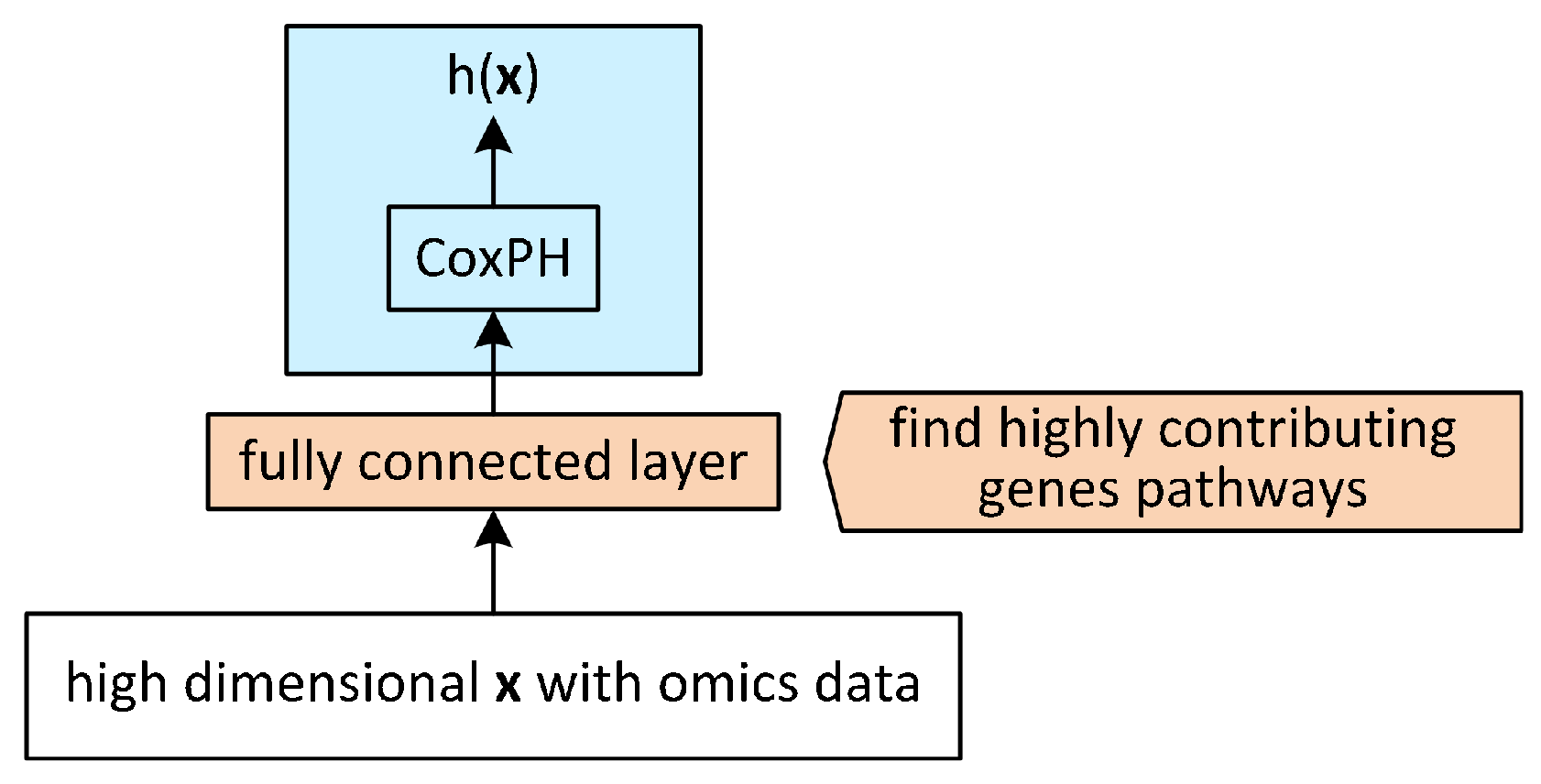
Cox–nnet [13] was developed for high throughput transcriptomics data and tested on 10 datasets, those containing at least 50 deaths, from The Cancer Genome Atlas (TCGA) [29]. The testing was performed alongside the algorithms from the main survival families: regression, forest, and boosting. The output of the NN with a single hidden layer enters the Cox regression model as an input (Figure 5). The set of hyperparameters was found via experimentation in 10-f cv. The method is biologically interpretable in the sense that input genes with high weights to the input nodes can be further analyzed with the methods designed to interpret gene function [30], such as the GO and KEGG.
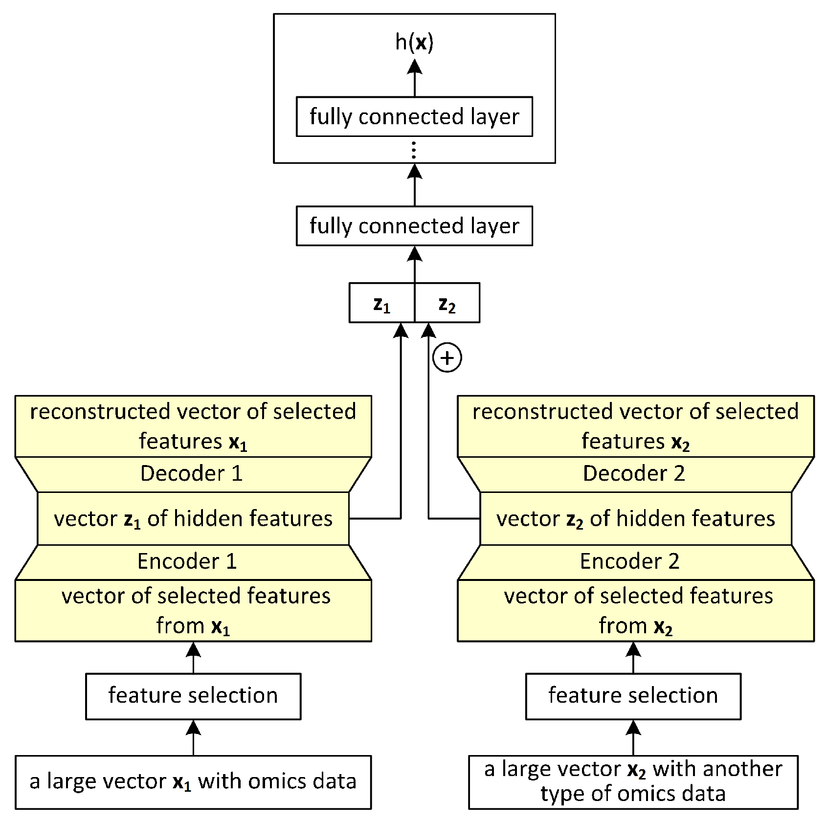
Concatenation autoencoders [19]: takes multi-omics data proven from breast cancer data from TCGA with 1060 patients and includes (1) gene expression, (2) miRNA expression, (3) DNA methylation, and (4) copy number variations. The number of attributes is made smaller via a supervised feature selection (Figure 6). The output of the fully connected neural network replaces the initial feature vector. Further, the fusion of different modalities is performed via a “concatenation autoencoder”, i.e., concatenating the hidden features learned from each modality, in this way benefiting from the idea that each modality brings unique information, emphasizing the complementarity principle. The idea of a cross-modality autoencoder is also considered (emphasizing agreement and achieving modality-invariant representation), but it is lower performing compared to the concatenation idea.
SurvivalNet [17] relies on the Bayesian optimization in order to automate the search of hyperparameter space. Testing is performed on the clinical and molecular data from TCGA: 17 K gene expression features and, additionally, other 3–400 features. The NN was fully connected (Figure 7). Among the ideas proposed is that deep survival models can successfully transfer information across diseases to improve prognostic accuracy: the dataset permits one to pretrain on and successfully transfer the parameters among different cancers. Interpretability is achieved via the interpretation of the weights of the features. A high C-index value of 0.8 is achieved, while the C-values reported by other studies are low (Table 2).
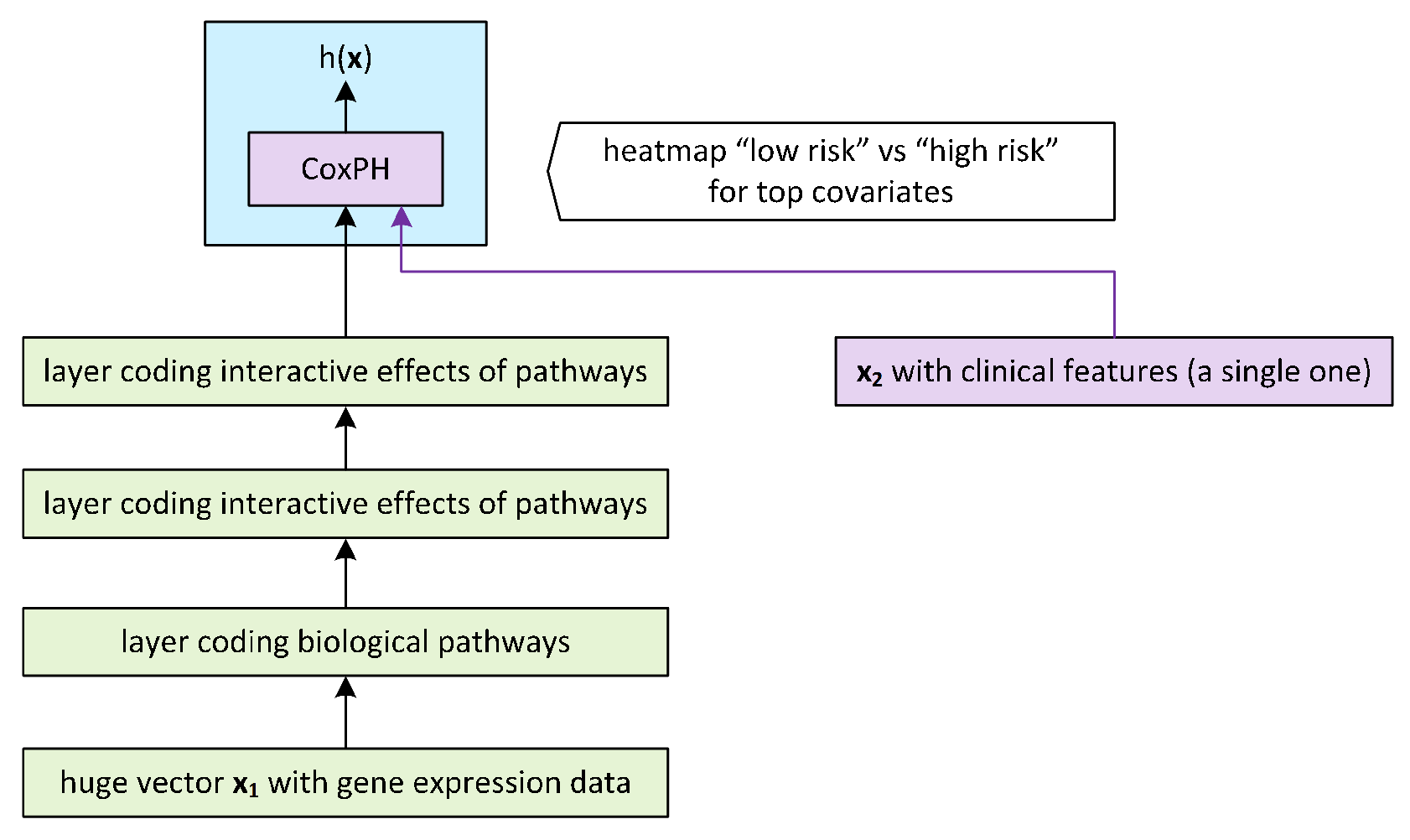
Cox-PASNet [18] works with 5.5 K genes (and 860 pathways) by 522 samples from the GBM dataset from TCGA. The architecture (Figure 8) incorporates biological knowledge and is comprised of the gene layer, followed by the pathway layer. There are multiple hidden layers also representing higher-level representations of biological pathways (as opposed to fully connected layers), and the Cox layer to which a clinical layer of one feature (age) is connected directly. The training is performed with sparse coding. In more recent work [31], the idea was expanded to fill the gaps in prior biological knowledge and expand the known pathways.
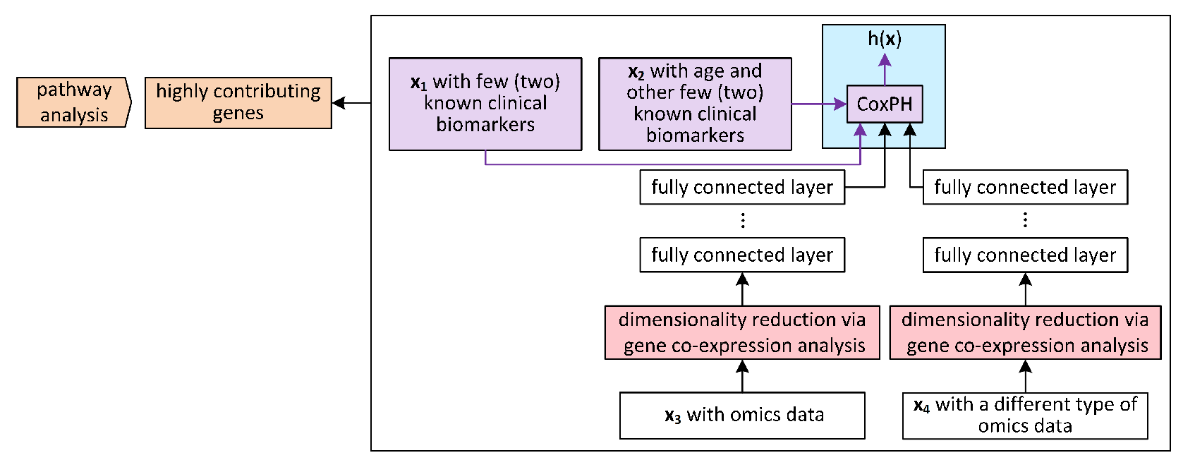
Survival Analysis Learning with Multi-Omics Neural Networks, SALMON [11], was tested on the data from 583 patients with breast cancer Figure 9. Diverse omics data were used, and the sets (available as supplementary files in the primary research article) were compiled by the authors with a subsequent 99% reduction of the input features. The model was trained on co-expression module eigen-genes instead of raw mRNA-seq and miRNAseq to reduce vector dimensionality with the number of resulting features <100, with few clinical variables connected directly to the Cox layer; the tuning of the DNN architecture is not detailed. The feature interpretation was achieved via removing the feature and checking whether the performance decreased: the larger the loss in performance, the more important the feature. The final layer implemented CoxPH. The rationale and the contribution was to develop methods to learn new attributes to confirm the known clinical information and reveal new knowledge. The authors of several articles stated that they are aware of this method and could have applied it [32].
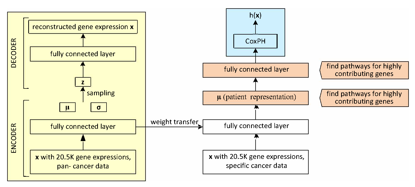
VAE-Cox [12] takes the transcriptomics data from 20 datasets of TCGA. The problem of p >> n is addressed via pretraining, namely, the low level weights are learned from other datasets. The optimal architecture is found via experimentation. The initialization weights are taken from the encoder model, which learns to map genes to genes. The third hidden unit is the input to the hazard ratio calculation. The contribution of the individual gene expressions to the disease is interpreted via the gene ontology analysis (KEGG): one layer learns disease-specific information and reveals pathways in cancer, and the other one is biologically basic and relates to metabolism only. The architecture is depicted in Figure 10. This is not used in clinical studies at the moment of the manuscript preparation.

4.3. Performance Comparison

The central success metric in survival analysis is the C-index, which approximates the area under the ROC curve (AUC). Typically, high values of C > 0.8 are needed to prove the validity of a new clinical biomarker [9].
As can be seen from Table 1 and Table 2, almost no method outperformed the Cox model by a large margin. Despite removing the technical flaws present in some earlier works, such as adding automatic tuning of hyperparameters (for the number of hidden layers, number of nodes in each layer, learning rate, the activation function), as well as achieving a high overall C-index on a realistically small databases, beating the Cox model remains not easy, e.g., [33] reported that it outperformed their best neural architecture.

5. Discussion

Several reusable traits can be noticed across the architectures.
Trait 1: In the Cox model, typically, few known to be important covariates (e.g., sex and age) are included alongside other covariates. In a neural architecture this is achieved via skip connections, namely, direct connections from these input features to high-level nodes. For example, x 1 and x 2 with relevant patient and clinical attributes are directly connected to h ( x ) in [11]. The same architectural decision is made in [14,18]. The corresponding parts of the architecture are highlighted with purple.
Trait 2: Fully connected architectures working on the omics features can be replaced with the ones constrained by the biological knowledge in the style of [18]. (For more variants, an interested reader is referred to a review on biologically informed neural networks [34]). Whenever the performance is comparable, the latter is the preferred type of the architecture over the fully connected counterpart due to its inherent interpretability. The corresponding part of the architecture is highlighted with green. Regarding the concrete works, there is some disagreement with respect to the performance of the knowledge-constrained vs. fully connected methods (underlined text in Table 2).
Trait 3: The analysis methods essential to bioinformatics for understanding and visualizing gene enrichment via gene ontology (e.g., with KEGG or GO) are applicable at the higher levels of the NN architectures to analyze the embeddings obtained via a neural network. The corresponding part of the schemes is highlighted with orange. The idea was applied in [11,12,13].
Trait 4: The notion of “eigen-gene” with the objective of dimensionality reduction can be integrated at the lower level of the neural network [11].
Trait 5: An independent classification or coding problem can become a part of the architectures, and its solution reinforces the main branch of computation with the weight transfer as in [12,19,28]. The corresponding parts of the architecture are highlighted in yellow.

6. Conclusions

RQ1: Does the DL component lead to notably improved performance? Unlike for images, for omics and clinicopathological covariates, a DL-based variant does not necessarily lead to a notably higher value of the success metric as compared to the Cox model.
RQ2: Are there any benefits of the deep-based survival that are not directly attainable with non-deep methods? There are several DL-specific advantages, including (a) a new type of interpretability, for example, via the architectures constrained with biological knowledge about genes and how they are organized into pathways, (b) biomarkers based on hundreds of weak covariates may potentially be constructed when no economic biomarker is available, and (c) gaining part of the solution in terms of weights from connected and already solved problems via transfer learning.
RQ3: Is there a new “gold standard” already for survival analysis with models implementing a neural network? The critical mass of technical research has been reached, in the sense that the DL-based survival methods have been applied in routine mission critical analysis published in central clinical journals (in 2023 for the selected articles), but statistical analysis as with the Cox glmnet() library in R remains the most used.
Having formulated the answers to the research questions, we should recall that the study was not based on an exhaustive search of the primary research articles on deep-based survival algorithms. By the question formulation, the first two answers are not affected by this limitation. The third answer can be biased by diminishing the importance of the new survival paradigm via having missed the uses of the not included methods. Yet, the point here is that deep methods have already appeared in clinical journals as part of clinical (not methodological) research.
The answer to RQ2, argument (b) implies higher costs of the sanitary system to measure the expression of hundreds of genes.

Author Contributions

The authors contributed equally: to the conceptualization J.S. and J.J.L., methodology J.S. and J.J.L., formal analysis J.S. and J.J.L., investigation J.S. and J.J.L., resources J.S. and J.J.L., data curation J.S. and J.J.L., writing—original draft preparation J.S. and J.J.L., writing—review and editing J.S. and J.J.L., and visualization J.S. and J.J.L. All authors have read and agreed to the published version of the manuscript.

Funding

This research received no external funding.

Acknowledgments

The authors thank the referees for the helpful comments.

Conflicts of Interest

The authors declare no conflicts of interest.

References

  1. Lin, Y.C.; Salleb-Aouissi, A.; Hooven, T.A. Interpretable prediction of necrotizing enterocolitis from machine learning analysis of premature infant stool microbiota. BCM Bipoinformatics 2022, 23, 104. [Google Scholar] [CrossRef] [PubMed]
  2. Efron, B.; Hastie, T. Computer Age Statistical Inference; Chapter 9 for Survival Analysis; Cambridge University Press: Cambridge, UK, 2021. [Google Scholar]
  3. Faraggi, D.; Simon, R. A neural network for survival data. Stat. Med. 1995, 14, 72–73. [Google Scholar] [CrossRef]
  4. Wiegrebe, S.; Kopper, P.; Sonabend, R.; Bender, A. Deep learning for survival analysis: A review. Aritificial Intell. Rev. 2024, 57, 65. [Google Scholar] [CrossRef]
  5. Sidorova, J.; Lozano, J.J. Need for Quality Auditing for Screening Computational Methods in Clinical Data Analysis, Including Revise PRISMA Protocols for Cross-Disciplinary Literature Reviews. In Proceedings of the International Conference on Advanced Research in Technologies, Information, Innovation and Sustainability, Madrid, Spain, 18–20 October 2023; Springer: Cham, Switzerland, 2023; pp. 133–142. [Google Scholar]
  6. James, G.; Witten, D.; Hastie, T.; Tibshirani, R. An introduction to Statistical Learning; Chapter 11 for Survival Analysis and Censored Data; Springer: New York, NY, USA, 2021. [Google Scholar]
  7. Kalbfleish, J.D.; Schaubel, D.E. Fifty years of the Cox Model. Annu. Rev. Stat. Appl. 2024, 10, 1–23. [Google Scholar] [CrossRef]
  8. Katzman, J.L.; Shaham, U.; Cloninger, A.; Bates, J.; Jiang, T.; Kluger, Y. DeepSurv: Personalised treatment recommender system using a Cox proportinal hazards deep neural network. BMC Med. Res. Methodol. 2018, 18, 24. [Google Scholar] [CrossRef]
  9. Sidorova, J.; Lozano, J.J. Commentary on “A systematic review on machine learning and deep learning techniques in cancer survival prediction”. Prog. Biophys. Mol. Biol. 2023, 174, 62–71. [Google Scholar]
  10. Zhou, H.; Wang, H.; Wang, S.; Zou, Y. SurvMetrics: An R package for predictive evaluation metrics in survival analysis. R J. 2022, 14, 252–263. [Google Scholar] [CrossRef]
  11. Huang, Z.; Zhan, X.; Xiang, S.; Johnson, T.S.; Helm, B.; Yu, C.Y.; Zhang, J.; Salama, P.; Rizkalla, M.; Han, Z.; et al. SALMON: Survival Analysis Learning with Multi-Omics Neural Networks on Breast Cancer. Front. Genet. 2019, 10, 166. [Google Scholar] [CrossRef] [PubMed]
  12. Kim, K.; Choe, J.; Lee, I.; Kang, J. Improved survival analysis by learning shared genomic information from pan-cancer data. Bioinformatics 2020, 36, i389–i398. [Google Scholar] [CrossRef]
  13. Ching, T.; Zhu, X.; Garmire, L.X. Cox-nnet: An artificial neural network method for prognosis prediction of high-thoughput omics data. PLoS Comput. Biol. 2018, 14, e1006076. [Google Scholar] [CrossRef]
  14. Yang, C.H.; Moi, S.H.; Ou-Yang, F.; Chuang, L.Y.; Hou, M.F.; Lin, Y.D. Identifying risk stratification associated with a cancer for overall survival by deep-learning based CoxPH. IEEE Access 2019, 7, 67708–67717. [Google Scholar] [CrossRef]
  15. Lee, C.; Zame, W.; Yoon, J.; Van Der Schaar, M. DeepHit: A Deep Learning Approach to Survival Analysis with Competing Risks. In Proceedings of the 32nd AAAI Conference on Artificial Intelligence, New Orleans, LA, USA, 2–7 February 2018; AAAI Press: Palo Alto, CA, USA, 2018. [Google Scholar]
  16. Kvamme, H.; Borgan, Ø.; Scheel, I. Time-to-event prediction with neural network and Cox regression. J. Mach. Learn. Res. 2019, 20, 1–30. [Google Scholar]
  17. Yousefi, S.; Amrollahi, F.; Amgad, M.; Dong, C.; Lewis, J.E.; Song, C.; Gutman, D.A.; Halani, S.H.; Velazquez Vega, J.E.; Brat, D.J.; et al. Predicting clinical outcomes from large scale cancer genomic profiles with deep survival models. Sci. Rep. 2017, 7, 11707. [Google Scholar] [CrossRef]
  18. Hao, J.; Kim, Y.; Mallavarapu, T.; Oh, J.H.; Kang, M. Cox-PASNet: Pathway-based sparse deep neural network for survival analysis. In Proceedings of the IEEE International Conference on Bioinformatics and Biomedicine (BIBM), Madrid, Spain, 3–6 December 2018; pp. 381–386. [Google Scholar]
  19. Tong, L.; Mitchel, J.; Chatlin, K.; Wang, M.D. Deep learning based feature-level integration of multi-omics data for breast cancer patients survival analysis. BCM Med. Inform. Decis. Mak. 2020, 20, 225. [Google Scholar] [CrossRef]
  20. Knaus, W.A.; Harrell, F.E.; Lynn, J.; Goldman, L.; Phillips, R.S.; Connors, A.F.; Dawson, N.V.; Fulkerson, W.J.; Califf, R.M.; Desbiens, N.; et al. The SUPPORT prognostic model: Objective estimates of survival for seriously ill hospitalized adults. Ann. Intern. Med. 1995, 122, 191–203. [Google Scholar] [CrossRef]
  21. Sahu, A.; Wang, X.; Munson, P.; Klomp, J.P.; Wang, X.; Gu, S.S.; Han, Y.; Qian, G.; Nicol, P.; Zeng, Z.; et al. Discovery of targets for immune-metabolic antitumor drugs identifies estrogen-related receptor alpha. Cancer Discov. 2008, 13, 672–701. [Google Scholar] [CrossRef]
  22. Chen, X.; Li, Y.X.; Cao, X.; Qiang, M.Y.; Liang, C.X.; Ke, L.R.; Cai, Z.C.; Huang, Y.Y.; Zhan, Z.J.; Zhou, J.Y.; et al. Widely targeted quantitative lipidomics and prognostic model reveal plasma lipid predictors for nasopharingal carcinoma. Lipids Health Dis. 2023, 22, 81. [Google Scholar] [CrossRef]
  23. Luo, L.; Tan, Y.; Zhao, S.; Yang, M.; Che, Y.; Li, K.; Liu, J.; Luo, H.; Jiang, W.; Li, Y.; et al. The potential of high-order features of routine blood test in predicting prognosis of non-small cell lung cancer. BCM Cancer 2023, 23, 496. [Google Scholar] [CrossRef]
  24. Thernau, T.M.; Grambsch, P.M. Modeling Survival Data: Extending the Cox Model; Version 2.38; Springer: New York, NY, USA, 2000; ISBN 0-387-98784-3. [Google Scholar]
  25. Sonabend, R.; Király, F.J.; Bender, A.; Bischl, B.; Lang, M. mlr3proba: An R package for machine learning in survival analysis. Bioinformatics 2021, 37, 2789–2791. [Google Scholar] [CrossRef]
  26. Schulze, J.B.; Durante, L.; Günther, M.P.; Götz, A.; Curioni-Fontecedro, A.; Opitz, I.; von Känel, R.; Euler, S. Clinically Significant Distress and Physical Problems Detected on a Distress Thermometer are Associated with Survival Among Lung Cancer Patients. J. Acad. Consult. Liaison Psychiatry 2023, 64.2, 128–135. [Google Scholar] [CrossRef]
  27. SEER Cause—Specific Death Classification. Available online: https://seer.cancer.gov/causespecific/ (accessed on 1 April 2024).
  28. Yang, F.O.; Hsu, N.C.; Moi, S.H.; Lu, Y.C.; Hsieh, C.M.; Chang, K.J.; Chen, D.R.; Tu, C.W.; Wang, H.C.; Hou, M.F. Efficacy and toxicity of pegylated liposomal doxorubicin-based chemotheraphy in early-stage breast cancer: A multicenter retrspective case-control study. Asia Pac. J. Clin. Oncol. 2018, 14, 198–203. [Google Scholar] [CrossRef] [PubMed]
  29. Grossman, R.L.; Heath, A.P.; Ferretti, V.; Varmus, H.E.; Lowy, D.R.; Kibbe, W.A.; Staudt, L.M. Toward a shared vision for cancer genomic data. N. Engl. J. Med. 2016, 375, 1109–1112. [Google Scholar] [CrossRef] [PubMed]
  30. Lin, C.; Jain, S.; Kim, H.; Bar-Joseph, Z. Using neural networks for reducing the dimensions of single-cell RNA-Seq data. Nucleic Acids Res. 2017, 45, e156. [Google Scholar] [CrossRef]
  31. Hou, Z.; Leng, J.; Yu, J.; Xia, Z.; Wu, L.Y. PathExpSurv: Pathway expansion for explainable survival analysis and disease gene discovery. Bioinformatics 2023, 24, 434. [Google Scholar] [CrossRef] [PubMed]
  32. Hu, F.; Zeng, W.; Liu, X. A gene signature of survival prediction for kidney renal cell carcinoma by multi-omic data analysis. Int. J. Mol. Sci. 2019, 20, 5720. [Google Scholar] [CrossRef] [PubMed]
  33. Alinia, S.; Asghari-Jafarabadi, M.; Mahmoudi, L.; Norouzi, S.; Safari, M.; Roshanaei, G. Survival predicion and prognostic factors in colorectal cancer after curative surgery: Insights from cox regression and neural networks. Sci. Rep. 2023, 13, 15675. [Google Scholar] [CrossRef]
  34. Wysocka, M.; Wysocki, O.; Zufferey, M.; Landers, D.; Freitas, A. A systematic review of biologically-informed deep models for cancer: Fundamental trends for encoding and interpreting oncology data. BCM Bipoinformatics 2023, 24, 198. [Google Scholar] [CrossRef]
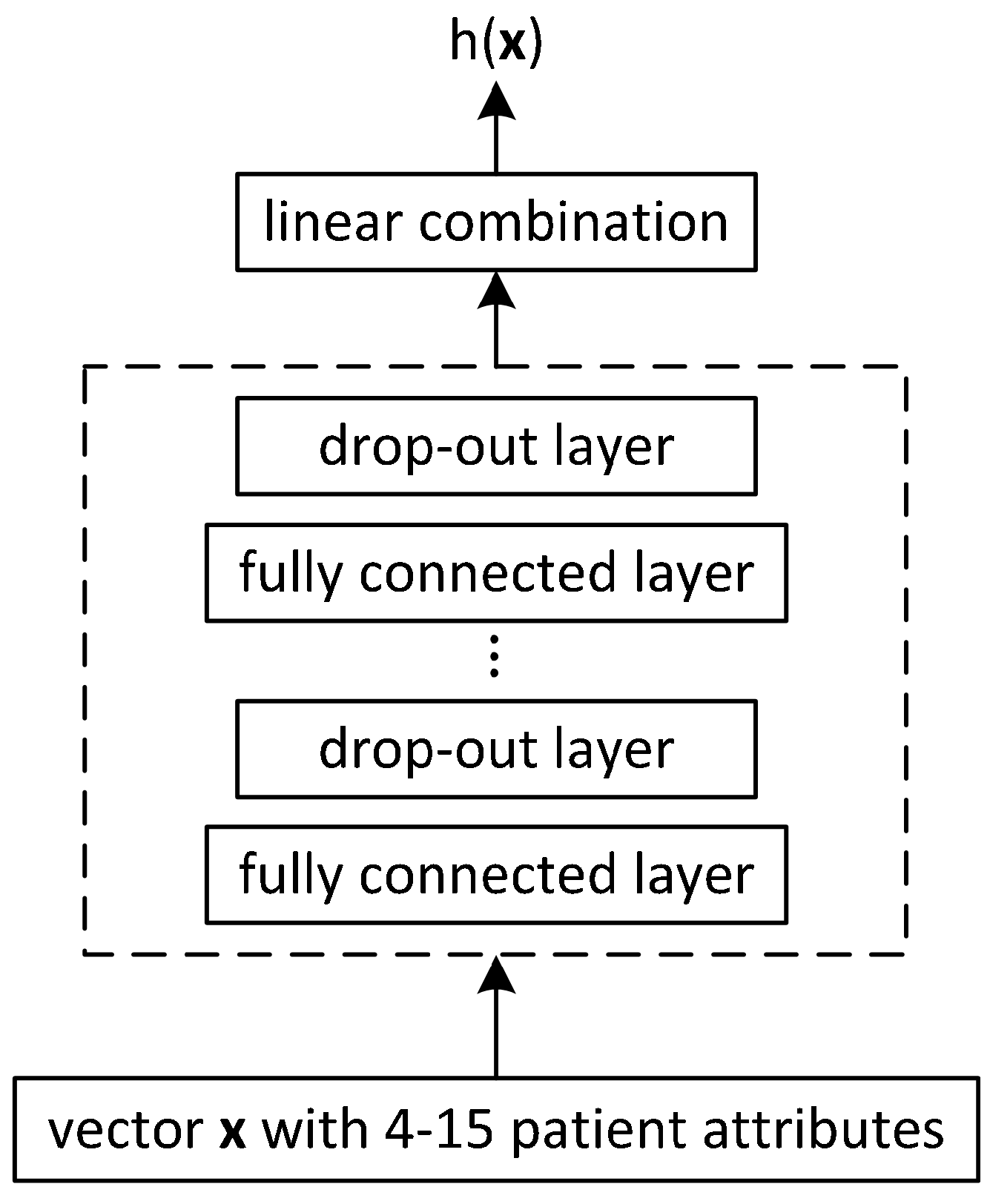
Figure 1. The neural architecture of the DeepSurv [8].
Inventions 09 00059 g001
Figure 2. The neural architecture of the Cox-CC-Time [16].
Inventions 09 00059 g002
Figure 3. The neural architecture of the DeepHit [15].
Inventions 09 00059 g003
Figure 4. The neural architecture of the DeepCoxPH [14].
Inventions 09 00059 g004
Figure 5. The neural architecture of the Cox–nnet [13].
Inventions 09 00059 g005
Figure 6. The neural architecture of the concatenation autoencoders [19].
Inventions 09 00059 g006
Figure 7. The neural architecture of the SurvivalNet [17].
Inventions 09 00059 g007
Figure 8. The neural architecture of the Cox-PASNet.
Inventions 09 00059 g008
Figure 9. The neural architecture of the SALMON [11].
Inventions 09 00059 g009
Figure 10. The neural architecture of the VAE-Cox [12].
Inventions 09 00059 g010
Table 1. The architectures tested on large datasets with few clinicopathological variables. (For references about the relation of C t d and C-index, see [16].
AlgorithmCommon DatabasesC-IndexPerformance Comparison
DeepSurv [8]SUPPORT, METABRIC, Rot&GBSD0.62, 0.65, 0.68CPH (=0.58) < DeepSurv;
CPH (=0.63) < DeepSurv;
CPH (=0.65) < DeepSurv.
Cox-CC-Time [16]SUPPORT, METABRIC, Rot&GBSD0.62, 0.66, 0.67 1CPH (=0.6) < DeepSurv < CoxTime (=0.63) < DeepHit; CPH (=0.63) < DeepSurv < CoxTime(=0.66) < DeepHit; CPH (=0.67) < DeepSurv < CoxTime (=0.68).
DeepHit [15]METABRIC0.69CPH (=0.65) = DeepSurv < DeepHit.
1 The C t d -index in place of the C-index for this row.
Table 2. The architectures working on the output of omics platforms, tested on the TCGA [29]. The contradictory results are underlined. The p-values of the comparisons are not taken into account.
AlgorithmCommon DatabasesC-IndexPerformance Comparison
Cox-nnet [13]10 datasets from TCGA, those with at least 50 deaths, gene expression On 4 out of 10 databases CoxPH (0.67) < Cox-nnet, while for the overall comparison the improvement with Cox-nnet is small (<0.02) yet statistically significant.
Concatenation autoencoders [19]Breast cancer data (BRCA) from TCGA, modalities: gene expression, miRNA, DNA methylation, and copy number variations0.64Concatenation autoencoders ≈ Cox-nnet (slightly) < CoxPH (if taken to be 0.675 as reported by [13])
SALMON [11]BRCA from TCGA with five omics data types incl. gene expression, miRNA, DNA methylation, and copy number variationsMedian concordance index of 0.72CoxPH (0.65) < Cox-nnet < SALMON
VAE-Cox [12]Same data as in [13]0.65VAE-Cox (0.66) is slightly < Cox-nnet
Cox-PASNet [18]GBM from TCGA, gene expression0.64CoxPH (glmnet) < SurvivalNet 1 < Cox-nnet < Cox-PASNet (0.65), the order as reported in [18].
SurvivalNet [17]GBM, BRCA, KIPAN from TCGA with different set of features: (1) 17K gene expression features, and (2) the set including 3–400 clinicopathological attributes, mutations, gene- and chromosome arm-level copy number variations, and protein expression.>0.8On GBM, PASNet < SurvivalNet (>0.8), the order as reported in [17]. On BRCA, SurvivalNet < Cox-nnet (0.67)
1 The contradictory data from the primary research articles are underlined.
Disclaimer/Publisher’s Note: The statements, opinions and data contained in all publications are solely those of the individual author(s) and contributor(s) and not of MDPI and/or the editor(s). MDPI and/or the editor(s) disclaim responsibility for any injury to people or property resulting from any ideas, methods, instructions or products referred to in the content.