Article

Investigations on Using Intelligent Learning Techniques for Anomaly Detection and Diagnosis in Sensors Signals in Li-Ion Battery—Case Study

1
Department of Engineering Technologies, John Abbott College, Sainte-Anne-de-Bellevue, Quebec, QC H9X 3L9, Canada
2
Department of Building, Civil and Environmental Engineering, Concordia University, Montreal, QC H3G 1M8, Canada
3
Department of Mathematics and Computer Science, University of Petrosani, 332006 Petrosani, Romania
4
Department of Mechanical Industrial and Transportation Engineering, University of Petrosani, 332006 Petrosani, Romania
*
Author to whom correspondence should be addressed.
Inventions 2023, 8(3), 74; https://doi.org/10.3390/inventions8030074
Submission received: 8 May 2023 / Revised: 17 May 2023 / Accepted: 19 May 2023 / Published: 22 May 2023

Abstract

:
This research paper aims to design and implement an intelligent least short time memory (LSTM) deep learning classification technique to detect possible anomalies in measurements dataset within a particular Li-ion battery type. For the state of charge (SOC) and battery faults estimation, a Joint State and Parameter Extended Kalman Filter (JEKF) estimator is developed. The SOC accuracy performance is excellent, with less than 0.5% error during steady-state, compared to the 2% error reported in the literature. For the design and implementation of JEKF SOC and parameter estimation is chosen a preset Li-ion battery Simulink Simscape generic model. It is also helpful to generate the healthy and faulty measurement dataset to design and implement the proposed intelligent LSTM classifier deep learning technique. The generic Li-ion battery model is wisely selected for the “proof concept” purpose, model validation, and algorithms’ robustness, accuracy, and effectiveness. Compared to the traditional EKF fault diagnosis and isolation (FDI), a model-based estimation strategy, the proposed classification LSTM technique is an intelligent data-driven-based deep learning algorithm of high accuracy (around 80%) and loss performance close to zero. Therefore, this feature makes data collection of dataset measurements directly from Li-ion battery sensors possible, which is beneficial for generating online fault scenarios. Additionally, the LSTM deep learning technique can remarkably classify all detected anomalies with high accuracy, independent of battery model accuracy, uncertainties, and unmodeled dynamics. Also, high-performance accuracy root mean square error (RMSE) of 0.0588 (voltage fault), approximately 5.5 × 10 7 (healthy) and 8.87 ×   10 6 (current fault) for deep learning shallow neural network (DLSNN) reveals an obvious superiority of both compared to the traditional FDI estimation strategies.

1. Introduction

Today, more than ever, the energy crisis that is deepening increasingly imposes the need to inject into the interconnected national and international energy network alternative sources of clean, green energy, which in the shortest possible time will completely replace the sources of polluting energy [1]. Transportation is among our planet’s most widespread sources of climate pollution, especially in crowded cities [2]. Recent years have seen remarkable progress in urban transport, with the impressive growth of a wide range of electric vehicles (EVs)/hybrid electric vehicles (HEVs) on public roads [3]. However, to finally reduce the share of toxic gases in the atmosphere, in other words, “zero” emissions and transport as clean as possible, the share of electric vehicles on public roads will have to increase to 100%.
This goal must be achieved in the shortest possible time so that changing the attitude in which the planet’s population uses energy will significantly impact avoiding the worst effects of climate change. Furthermore, emissions from cars and trucks are not only harmful to our planet but also to our health, causing high-risk diseases and possibly premature death. A significant advantage of EVs is that they are more efficient in converting energy to power cars and trucks. Also, electricity, across the board, is cleaner and cheaper than vehicle fuel [3,4]. Another advantage of electric vehicles is that most can be recharged, a good solution for truck and bus fleets that regularly return to a central depot or end station. In addition, new charging solutions are possible by adding more public charging locations in shopping malls, parking lots and workplaces [4]. Electric utility infrastructure, therefore, has a vital role in making it easier for people to buy electric cars on a large scale. The lithium-ion (LiB) battery is the core of an EV and is one of the most suitable sources of electrical energy storage (EESS). It is recommended for its top features: low self-discharge, high energy and high-power density, tiny memory effect, lightweight, long lifespan, and environmental approachability [5,6]. It is worth remarking that the performance of an EV relies on the battery pack it runs on. The battery pack consists of multiple modules of cells connected in series, parallel or combination series-parallel, constituting the whole grid of a power source. As a vital component of the integrated Battery Management Systems (BMS) structure of EV, the battery pack must be managed appropriately through the hardware components (electronics circuitry of high complexity such as charger, controllers, switches, current, voltage, temperature sensors, data acquisition equipment, etc.), as well as the software components (i.e., battery and thermal models, state and parameters estimators, fault detection, diagnosis and isolation (FDDI) in battery sensors and actuators, artificial intelligence learning models (machine learning and deep learning) used for anomaly detection, cell balancing, PI current-constant voltage (CC-CV) modes control algorithms, battery fast charging algorithms, etc.) [5,6,7,8,9,10,11,12]. Since each battery cell has a different operational state in the module, it is essential to monitor every battery cell in the module, such as the temperature, discharging or charging current, terminal battery voltage, state of charge (SOC), state of health (SOH), state of energy (SOE), as well as anomalies detection in the sensor’s functionality [7,8,9,10,11,12,13]. Summarizing, a Battery Management System (BMS) is an “intelligent component of a battery pack responsible for advanced monitoring and management”, as mentioned in [12]. Besides, “it is the brain behind the battery and plays a critical role in its levels of safety, performance, charge rates, and longevity” [12]. This produces reliable, safe, and secure products [10,11,12,13].
The flow of this paper is organized into four broad sections, as follows. The last two subsections of Section 1 present some preliminaries on data acquisition equipment and Li-ion BMS architectures and a literature review of several traditional model-based and data-driven-based learning estimation and classification techniques. Section 2 details some aspects related to selecting a predefined Li-ion Cobalt battery type, developing a generic Simulink Simscape Rint model based on parameter values extracted directly from battery curves that match the manufacturers’ specifications, and its thermal. Model, MATLAB simulation results of the AEKF SOC estimator and terminal voltage prediction, and statistical criteria for performance evaluation. Section 3.1 developed a general model to generate the healthy, additive current, voltage, and temperature fault models and injection mechanisms for current and voltage faults. Estimating the battery SOC and the faults uses an accurate and robust JEKF state and parameter estimator. A residual-based procedure is integrated into the fault detection and diagnosis scheme to detect the time instances for the injection and removal of each fault. Finally, based on the fault signature matrix, the fault is diagnosed (classified). Section 3.2 is applied a driven-data-based deep learning shallow neural network (DLSNN) technique for anomaly detection into sensors’ measurement datasets. Section 3.3 introduces a Deep Learning Neural LSTM to classify anomalies in the sensor measurement dataset. Section 4 contains detailed discussions of the MATLAB simulation results obtained by comparing the traditional EKF estimator and the accuracy performance of DLSNN and LSTM, the conclusion of this work, and future work.

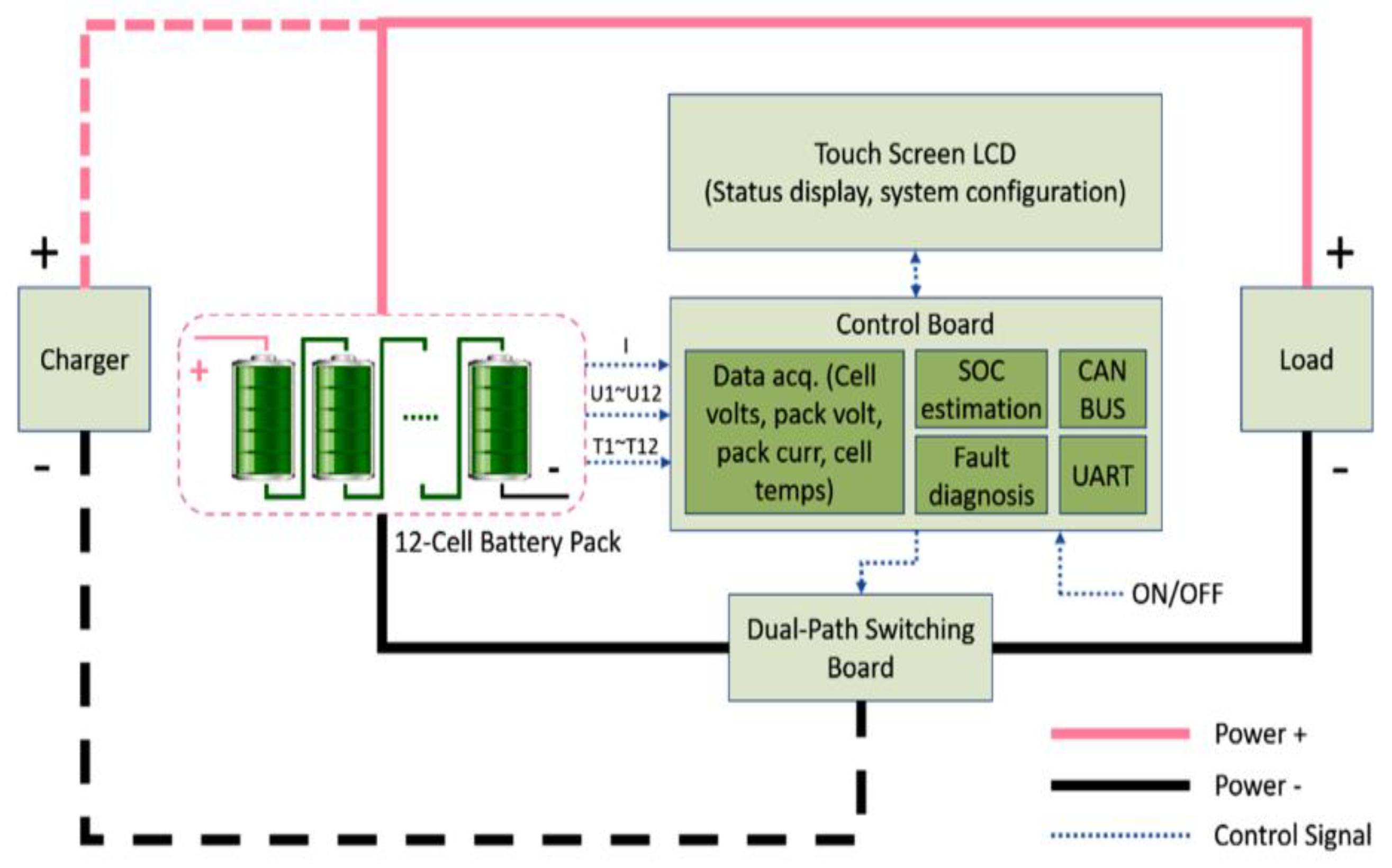
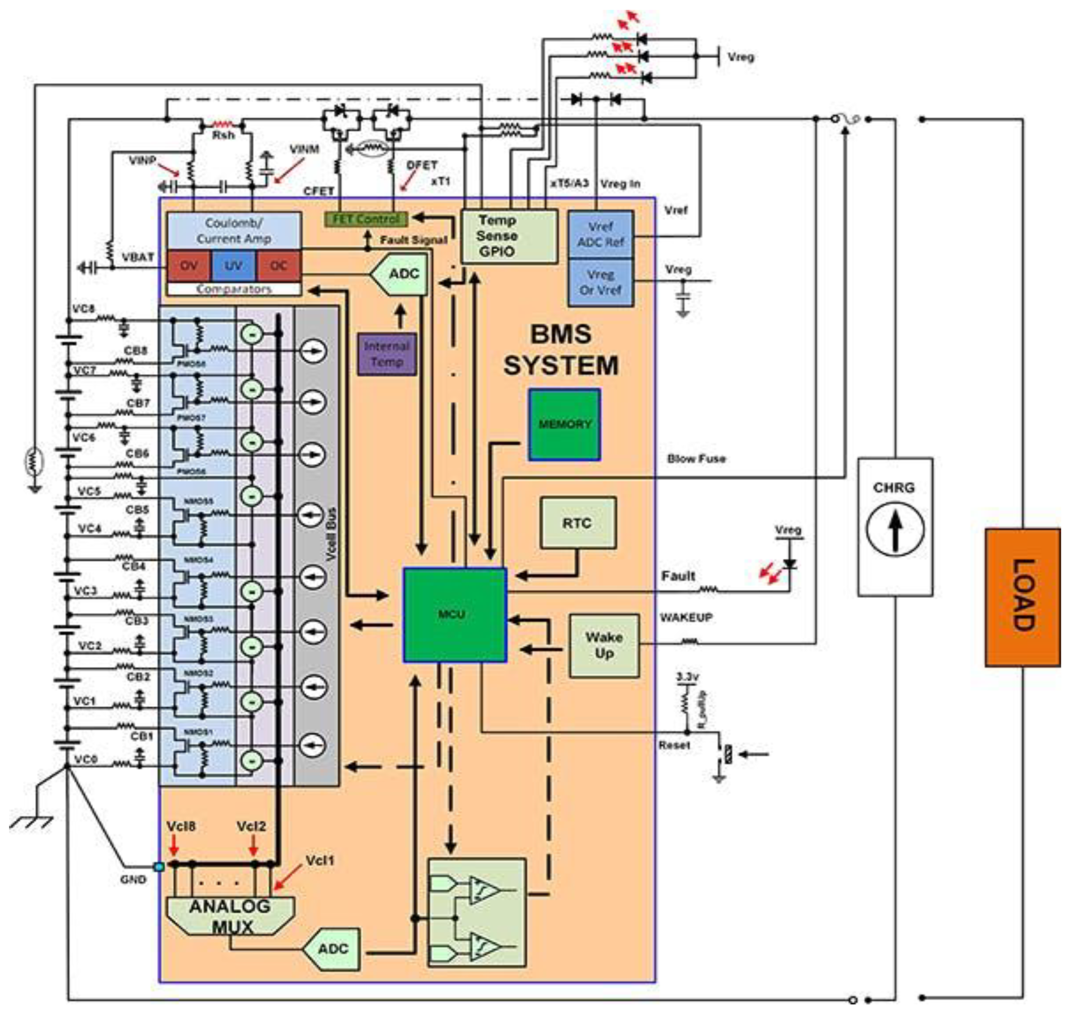
1.1. Preliminaries—Data Acquisition Equipment and BMS Architectures

Among the promising LIBs in the battery market, the most suitable and widespread for HEV/EV energy-storage applications are lithium-ion phosphate (LiFeO4), lithium polymer (LiPo) and lithium cobalt (LiCoO2) batteries [5]. An accurate SOC estimation of the battery in a BMS can improve its performance and reliability. Furthermore, to provide higher power density, the safety of the BMS power system in a LIB pack is crucial, as the battery could be damaged if used beyond the battery’s specifications [5]. An interesting simplified global system architecture of a smart battery power system is proposed in [5], which we reproduce in Figure 1 because it is well documented and provides enough detail to gain insight into the complexity of a LIB’s BMS. It integrates appropriate data acquisition (DAQ) equipment (sensors, analogue-to-digital converters (ADC)) to collect the values of charging/discharging voltages, currents, and temperatures for each battery cell, as well as for the entire particular battery pack consisting of 12-series cells. An appropriate LIB SOC estimator and real-time FDDI algorithms can be implemented based on these values. The specific values of LIB parameters such as “battery cell material, battery cell capacity, battery cell maximum discharge current, and battery topology” are provided by a touch LCD screen. Also, the LIB SOC estimated values and fault diagnosis results are displayed on the same LCD screen and sent further to a host computer via a Universal Asynchronous Receiver-Transmitter (UART) to be processed. For a battery pack larger than 12 cells, a controller area network (CAN bus) is required for communication with “other peer systems or the master system” [5].
A look inside a typical BMS architecture showing the main functional blocks such as field effect transmitters (FETs), fuel gauge, cells voltages, battery pack voltage and temperature monitors, cells voltage balance, real-time clock (RTC), and a state machine is depicted in Figure 2 reproduced from [14]. Some details about these functional blocks can be found on the Electronic Design website [14]. The research paper is focused only on the functional blocks related to battery SOC estimators and FDDI algorithms implemented in real-time and model-based, as well as anomaly detection algorithms in the functionality of the sensors based on input-output dataset measurements. Battery SOC is a critical internal state of the battery carefully monitored by the BMS as long as it seriously affects the health and life of the battery. It is well-defined as the battery’s remaining capacity at any service moment under different operating conditions, environments, and ambient temperatures [11]. It is well-known that during several charging and discharging cycles, the LIBs generate a significant amount of heat, which leads to an excessive increase in temperature inside the battery.
Temperature changes within the battery “not only damage the performance of the internal materials of the battery and reduce the service life of the battery, but also easily lead to overheating, expansion, electric leakage, fire, explosion, and other thermal runaway phenomena which pose a great threat to the safety of automobiles and passengers” [15,16].
A cooling and heating system must be installed to prevent the dangerous effects of temperature changes inside the battery and extend its life [11,15,16,17].
Since the SOC of the battery is significantly affected by the ambient environment and the temperature inside the battery, hysteresis effects, self-discharging, battery ageing effects during its service life, and sensitivity to the noise, it cannot be easily and accurately measured, and therefore the need to be estimated becomes a priority to prevent dangerous situations and improve battery performance [7,11,15,16,17]. In [18], accurate run-time SOC estimation techniques are used in BMS for “cell balancing of battery packs in vehicles with electrified powertrains”. Additionally, the battery SOC estimation “must be accurate under all vehicle operating conditions, and account for changes in temperature, different rates of current, and cell aging” [18].

1.2. Traditional Model-Based and Deep Learning Data-Driven-Based Models Estimation Techniques—Literature Review

The most used battery SOC estimation methods can be separated into three main categories, such as the Coulomb counting direct measurement method [18], model-based methods which simulate the battery internal structure, materials and chemical reactions of a battery by building a linear equivalent electric circuit model (ECM) and methods based on input-output data set measurements, well-known as data-driven methods, which analyze the historical data collected through laboratory measurements [9]. A simple SOC estimation method reported in the literature is the Coulomb counting method, an open-loop method with a time integrator (i.e., time accumulation effect) of the battery current during a charging/discharging cycle. The main flaw of the Coulomb counting SOC estimation method is that it “does not account for self-discharge currents or parasitic reactions in the cell” [18], and thus to prevent the accumulation in time of current measurement errors, “it should be corrected by periodic recalibration” [18]. A significant improvement of the Coulomb counting SOC estimation method is achieved in [19], an attractive feedback closed-loop SOC estimation approach, which uses a Li-ion battery cell model whose parameters are temperature dependent. A PI controller and the battery cell model (i.e., chosen as a plant) are connected in series in the forward path of a closed–loop feedback control system structure. The controller output is a voltage that “follows the measured battery cell voltage, which acts as the reference input of the closed–loop system” [19]. In this approach, the combined SOC estimation algorithm “requires less computational resources than other model-based approaches, such as Kalman filtering” [19]. Also, the model–based component of the integrated combined SOC estimation algorithm “basically corrects low–frequency errors induced to the Coulomb counting SoC estimation by offset temperature drifting of the current sensor” [19]. Furthermore, the combined SOC estimation algorithm gains robustness against an incorrect SoC guess compared to a simplified Coulomb counting method [19]. A similar combined Coulomb counting SOC approach in an adaptive estimation scheme connecting the battery cell dynamic model with an adjusted gain is developed in [20]. The field literature is awash with different approaches to improve the accuracy of SOC estimators, which remains a true challenge due to the “uncertainties involved, such as temperature, varying power requests, aging effects”, and so on, as mentioned in [21]. It is worth noting the three research papers [22,23,24] that reveal the first results of a high scientific value research in the field of Li-ion polymer (LiPo) batteries. These three fundamental research works develop model-based SOC estimation algorithms, the state-of-the-art Kalman filter (KF) SOC estimators, noting the two well-known versions spread in the literature, linear KF (LKF) and extended KF (EKF). Then similar approaches are extended to the nonlinear models developed to capture the entire dynamics of these models, such as the fundamental research work unscented KF (UKF) [25], as well as its new version, the square root UKF (SRUKF) [26], particle filter KF (PKF) SOC estimator [27]. It is worth noting that to design an accurate, robust, and optimal SOC estimator using a Kalman filter. It is necessary to possess in advance accurate information about the process and the measurement noise; otherwise, it would lead to a poor filter convergence rate, but a rather tricky task [28]. To overcome this drawback, a genetic algorithm for SOC estimation is developed in [28] based on a particle swarm optimization (PSO); a great advantage of this approach is that the requirement to linearize the non-linear battery model, as well as prior knowledge on measurement and process noise is no longer required. The main purpose of the genetic PSO SOC estimator is to determine the unknown parameters to obtain the battery open circuit voltage (OCV), which depends on the SOC of the battery and, therefore, using a lookup table, the SOC can be estimated. Finally, artificial intelligence (AI) data-driven based methods, using fuzzy logic, adaptive neural networks fuzzy inference system (ANFIS) models, machine learning (ML) and deep learning (DL) estimation methods adapted to li-ion batteries SOC estimation and prediction are reported in the literature [29,30,31]. Also, these SOC estimation techniques are adapted for fault detection and isolation or anomaly detection algorithms in the sensors and actuators functionality monitored in BMS [5,32,33,34,35,36,37,38,39,40,41,42,43]. Anomaly detection is a technique that uses AI to identify abnormal behavior compared to an established pattern. Anything that deviates from an established baseline pattern is considered an anomaly. Although the AI algorithms eliminate the impact of the nonlinearity of the battery model on the overall battery performance, the computational cost is still high, and significantly large training data are required to ensure the accuracy of state and parameter estimation.

2. Materials and Methods

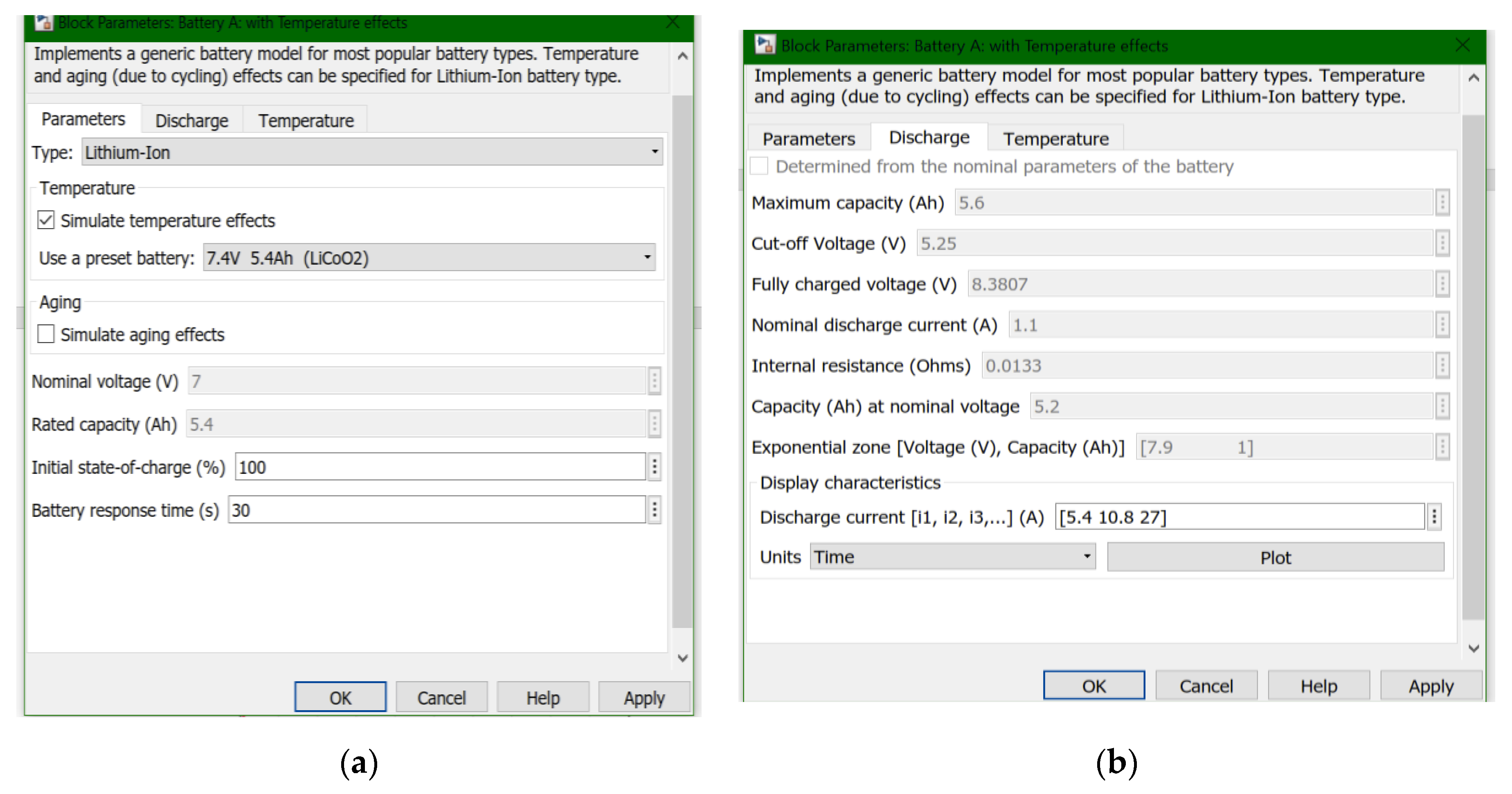
2.1. Li-Ion Model Selection and Simulink Simscape Block Setup

As a case study for implementing the design, models and methods of possible anomalies detection in the functionality of measurement sensors, for “proof concept” and simulation purposes, is adopted a simple Rint generic Simulink Simscape model of a preset 7.4 V nominal voltage and 5.4 Ah rated capacity Li-ion cobalt battery (LiCoO2) for possible integration in a Battery Management System of an HEV/EV [11].
As is shown in Figure 3, the battery model parameters can be extracted from the data specifications of a collection of generic SIMULINK Simscape battery models without temperature effects that match the manufacturers’ specifications. Therefore, the validation of the model is not necessary as long as the parameter values match the manufacturers’ specifications. However, calibration of the parameter values is required when is not a perfect match between the battery model SOC and the SOC generated by the Simulink Simscape block.
The ambient temperature for the battery is set to 20 °C. Figure 4a is presented the voltage discharge curve for a constant current (CC) discharge of 0.2037 C-rate, i.e., 1.1 A during an interval of 5.241 h discharging time. In Figure 4b are specified the generic battery model parameters (E0, R, K, A, B) that represent a constant voltage source (E0), the internal resistance of the battery cell (R), the polarization constant (K) and the last two parameters (A and B) define the exponential area (blue surface in Figure 4a). Also, in the same figure are represented three discharging voltage curves for 1C, 2C and 5C (CC) discharging rates, i.e., for constant discharging currents of 5.4 A, 10.8 A, and 27 A, respectively.
The generic Simulink Simscape Li-ion preset battery model type and its parameters, discharging current rates and temperatures setup are also specified in Figure 5a–c.

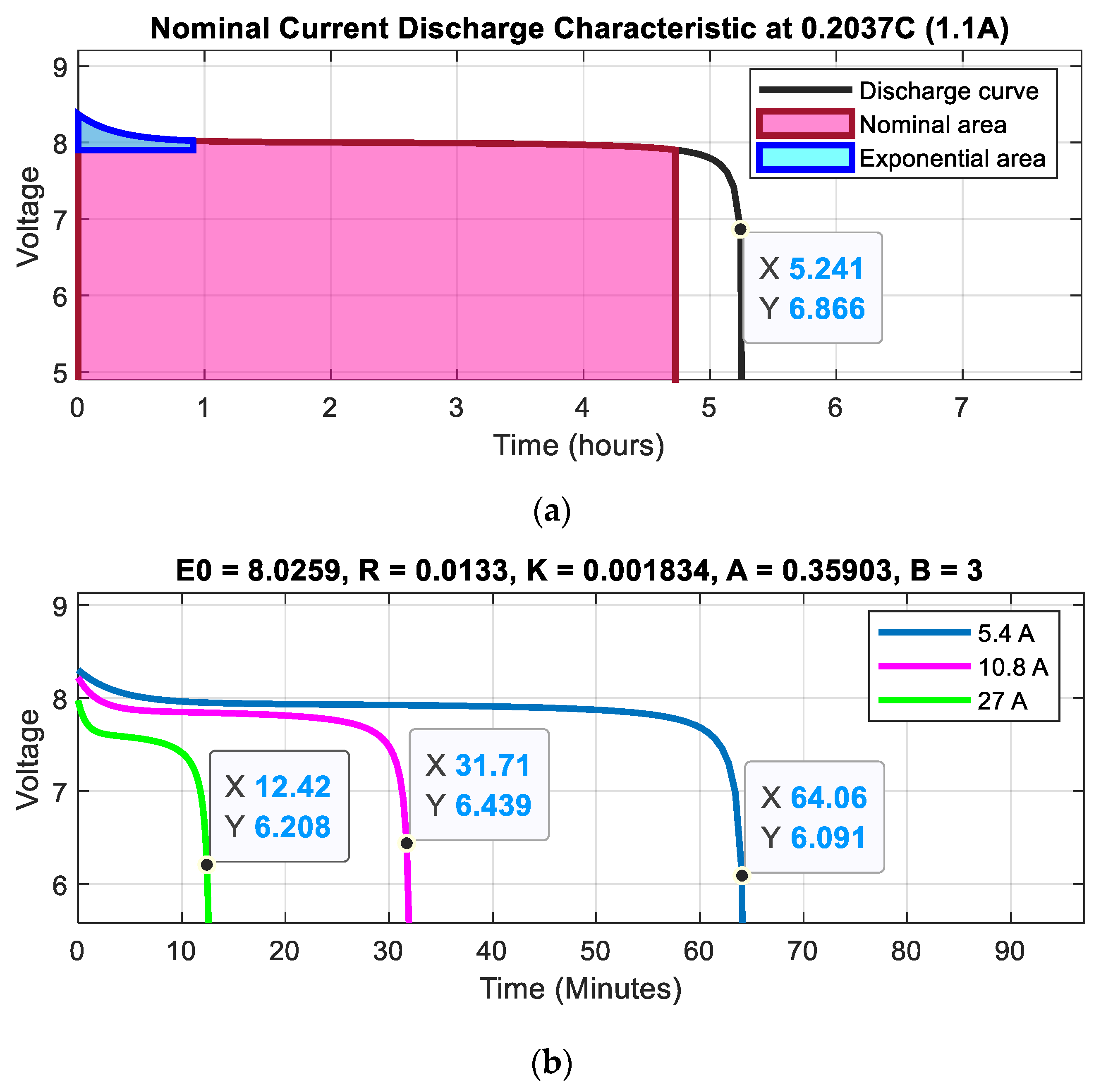
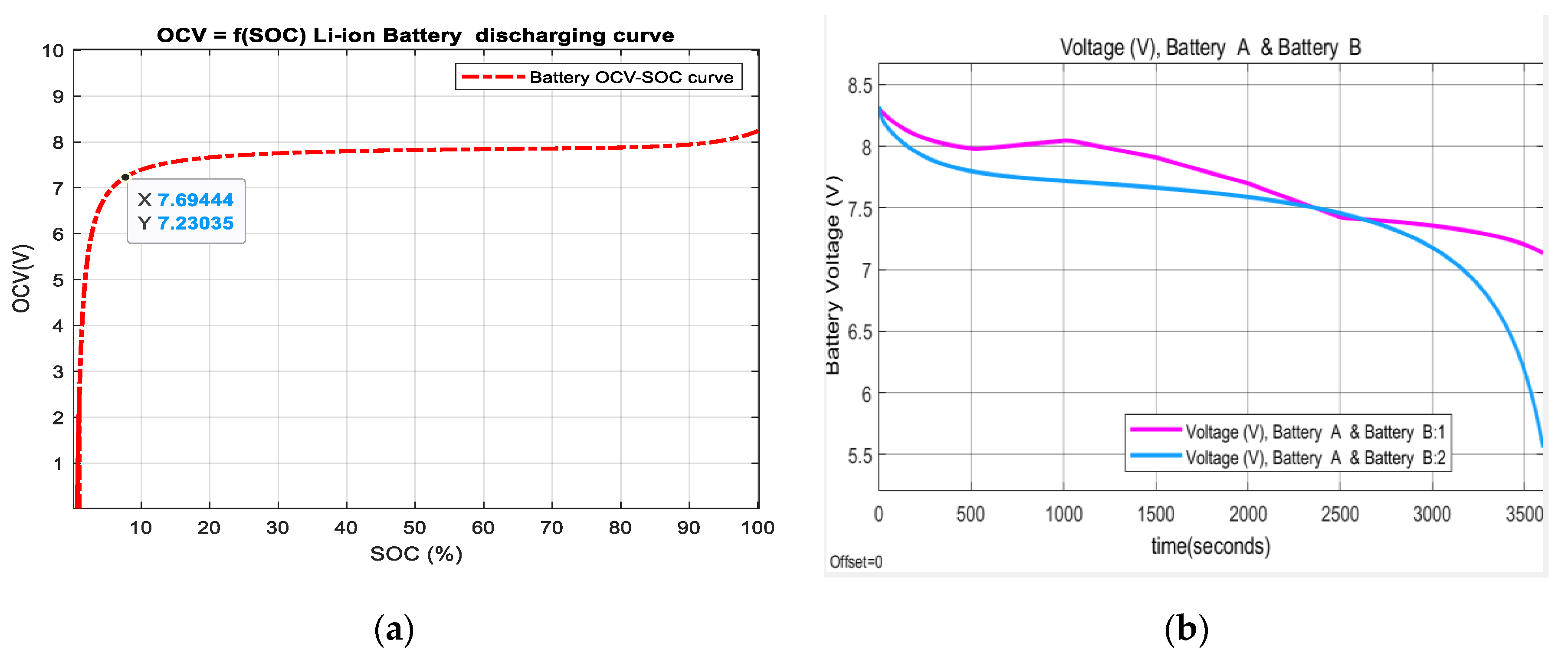
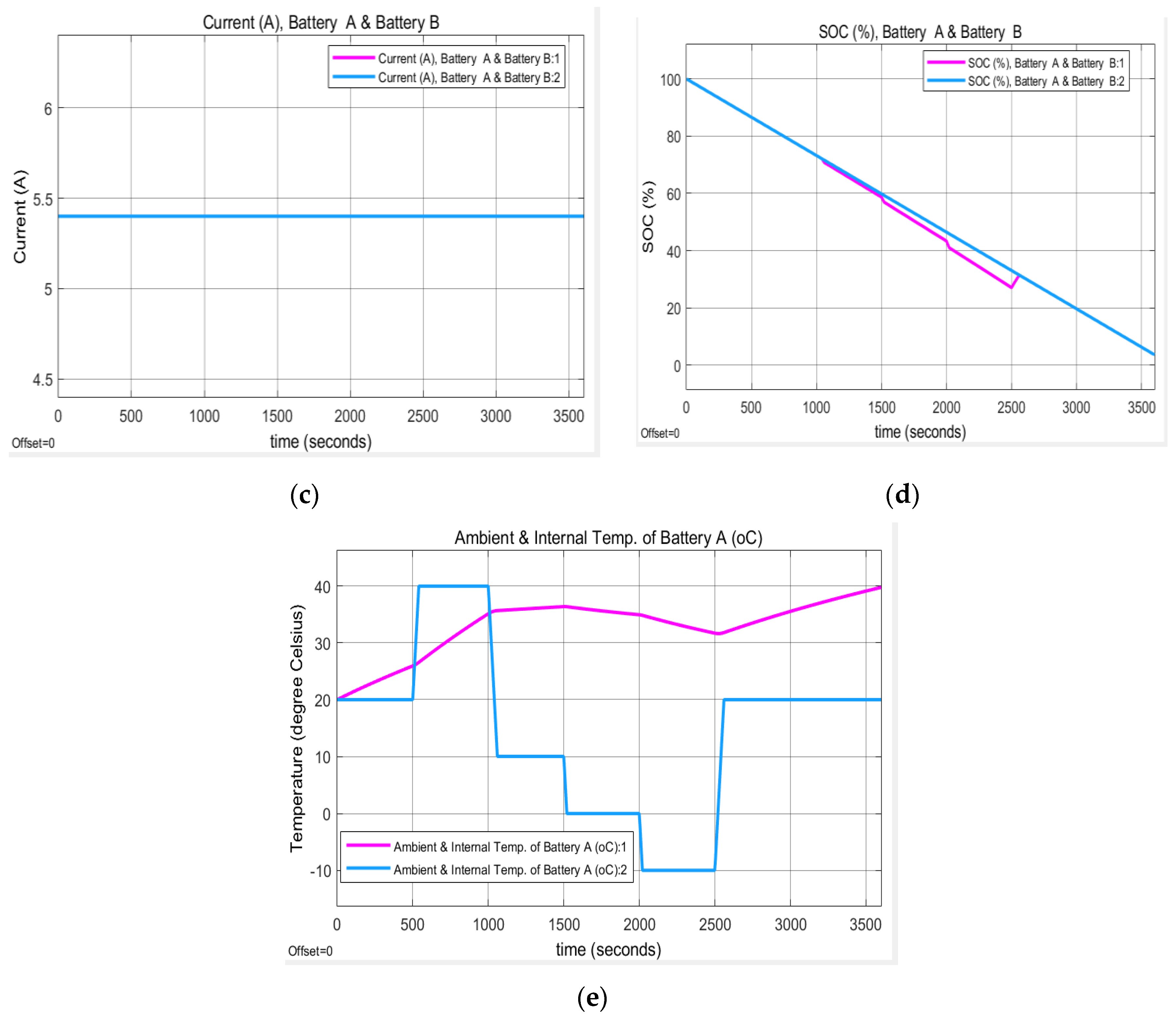
2.1.1. Li-Ion Cobalt Battery Type Model Performance with and without Temperature Effects

For particular settings of the Simulink Simscape battery block for a preset Li-ion battery selection shown in Figure 3, both batteries performance A and B can be visualized in Figure 6, namely the OCV = f(SOC) discharging curve (a), battery terminal cells voltages (b), CC battery discharging values within the cells (c), the SOCs battery cells (d), and the ambient and temperatures cells (e), provided through several simulations conducted in MATLAB Simulink R2019b software (MathWorks, Natick, MA, USA) environment.

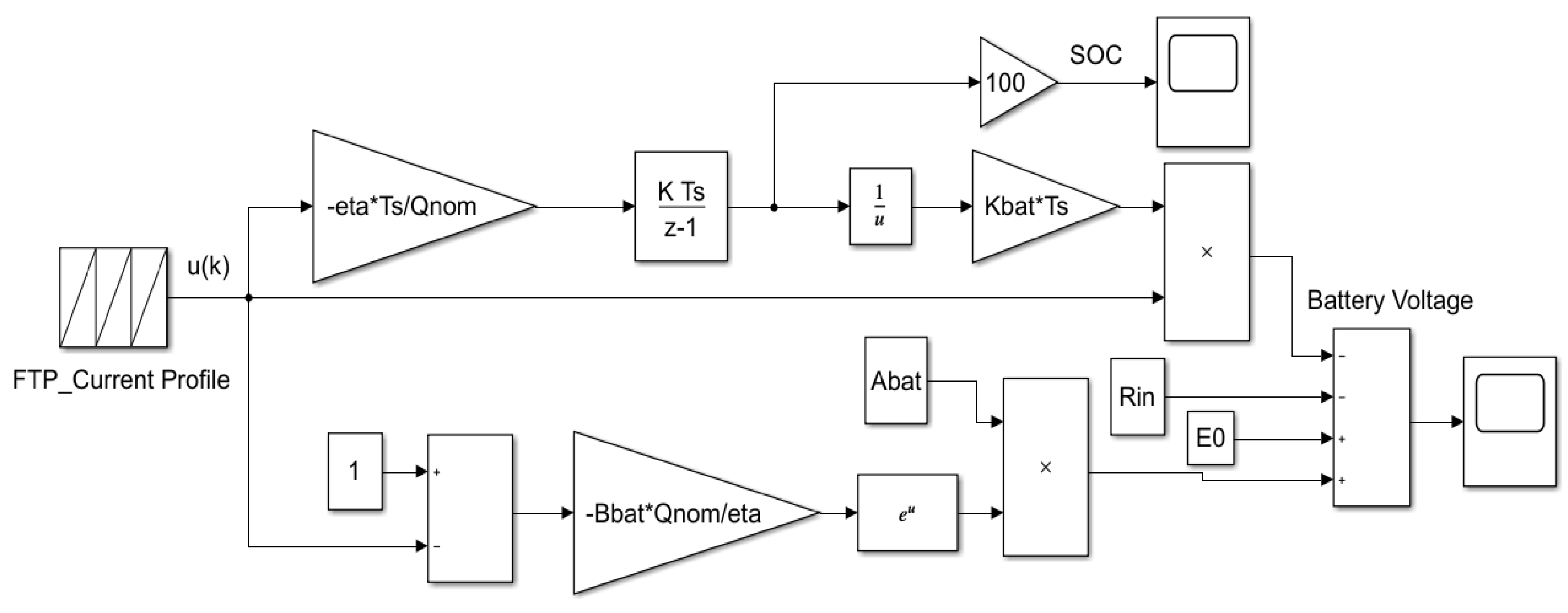
2.1.2. Li-Ion Cobalt Type Battery -Analytical Model

Based on the generic Simulink Simscape battery model parameters extracted from the nominal current discharge characteristic at CC 0.2037C rate, i.e., CC at 1.1 A, represented in Figure 4a,b, an accurate and simplified analytical battery model can fit a similar discrete-time unidimensional state space representation as the models developed in [10,11] given by the following two equations:
x 1 ( k + 1 ) = x 1 ( k ) T s ( η Q n o m ) × u ( k )
y ( k ) = E 0 K b a t T s x 1 ( k ) × u ( k ) + A b a t e x p ( B b a t Q n o m η ( 1 x 1 ( k ) ) ) R i n u ( k )
where x 1 ( k ) x 1 ( k T s ) = S O C ( k T s ) , u ( k ) ,   y ( k ) , Q n o m , η and T s designate the discrete-time battery SOC, input current cell, output battery terminal voltage, nominal battery capacity, a constant Coulomb charging and discharging efficiency value of 0.75, and sampling time, respectively.
The model parameters value suited to fit well is recalibrated and set to the following values: E 0 = 8.0259   [ V ] , R i n = 0.0133   [ ] (internal cell resistance), K b a t = 0.001834   [ V A s ] (polarization constant), A b a t = 0.35903 [ V ] , B b a t = 3 [ 1 / ( A h ) ] , T s = 1   [ s ] , Q n o m = 5.4   [ A h ] (nominal cell capacity), η = 0.75 , (Coulomb efficiency). It is essential to emphasize a great advantage of the adopted Simulink Simscape model, presented in Equations (1) and (2), consisting of a considerable model simplification and dependence only on SOC. Also, the dynamics of this model are described by the first Equation (1), which is linear, and the second Equation (2) is a highly nonlinear static representation. The Simulink Simscape diagram of the analytical Li-ion battery model that implements Equations (1) and (2) is shown in Figure 7 [11].

2.2. Anomaly Detection and Diagnosis Techniques for Li-Ion Battery—Additive Bias Faults within Voltage and Current Measurement Sensors

2.2.1. Joint State and Parameter EKF Estimation for Fault Detection and Diagnosis of Anomalies in LIB’s Sensors

Few state estimation strategies reported in the literature field refine online the model parametric uncertainties to improve the accuracy of state estimation. Such methodology is called joint state and parameter estimation, enabling simultaneous estimation of both states and model parameters [24]. For simplicity and “proof concept” and simulation purposes, in the case study, we present only two bias current and voltage sensor faults as the most spread in Li-ion battery (LIB) of an HEV’s BMS. However, for a complete description that delivers valuable information to the readers and implementers interested in new investigations, the Li-ion battery model is combined with the thermal battery model. Thus, it is helpful to study also the fault detection and diagnosis of a temperature sensor fault if the battery is not equipped with a control system of the battery temperature for kiping constant and uniform the temperature in each cell of the battery pack. All two faults are denoted by f I ,   f V respectively, attached to Equations (1) and (2), and also to the battery thermal model for an overall battery model, by addition or multiplication operations, and whose dynamics are described by the following discrete-time equations.
x 1 ( k + 1 ) = x 1 ( k ) T s ( η Q n o m ) × ( u ( k ) + f I ( k ) ) + w 1 ( k )
x 2 ( k + 1 ) = ( 1 T s T c ) ( x 2 ( k ) ) + T s T c × T r e f ( k ) + T s R t h R i n ( k ) T c ( u ( k ) + f I ( k ) ) 2 + w 2 ( k )
f I ( k + 1 ) = f I ( k ) + w I ( k )
f V ( k + 1 ) = f V ( k ) + w V ( k )
( k ) = E 0 K b a t T s x 1 ( k ) × ( u ( k ) + f I ( k ) ) + A b a t e x p ( B b a t Q n o m η ( 1 x 1 ( k ) ) ) R i n ( k ) ( u ( k ) + f I ( k ) ) + f V ( k ) + v 1 ( k )
and R i n ( k ) is temperature dependent according to Equation (5). The absence of the fault will be sensed when f I ,   f V will be equal to zero, and their presence when the value is equal to 1 or greater than zero for f V .
In all the Equations (5)–(10), the variables w 1 ( k ) ,   w 2 ( k ) , w I ( k ) , w V ( k ) and v 1 ( k ) represent the Gaussian process noises and measurement noise, respectively, assumed that all are uncorrelated. In this development, the faults appear as joint parameters attached to both states SOC and Temperature, whose values will be estimated using the same previous AEKF algorithm, whose steps are summarized in Annex A of [37].

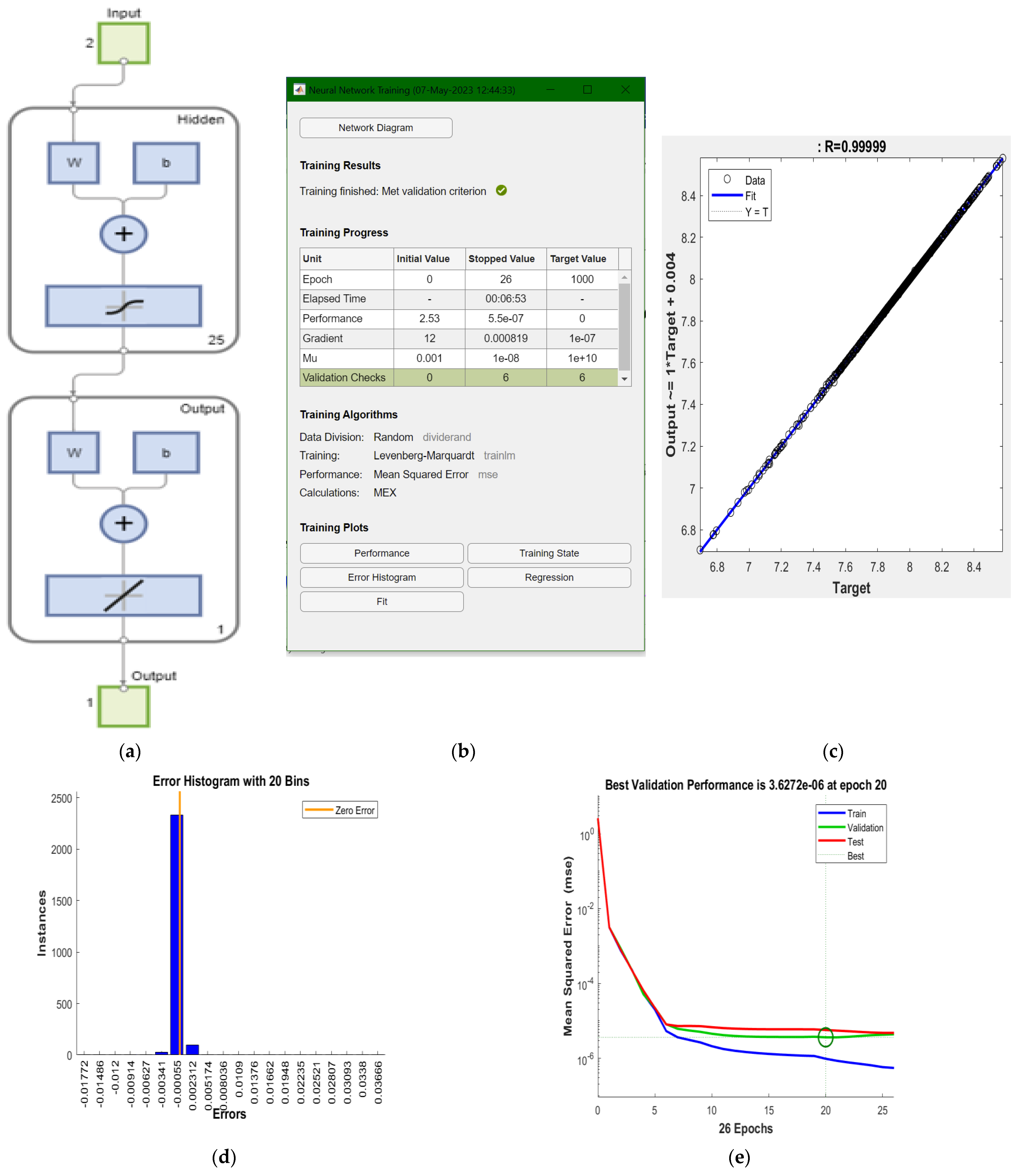
2.2.2. Data-Driven-Based Deep Learning Shallow Neural Network for Anomaly Prediction into Sensors’ Measurement Dataset

To predict the sequence of health, voltage, and current anomalies (faults) based only on the input-output data set of measurements collected from the voltage and current sensors, an exciting alternative to the traditional model-based EKF SOC estimator is to use a simple Deep Learning Shallow Neural Network (DLSNN) with an input layer with two inputs, current (FTP-75 driving profile) and battery SOC (Predictors, P), a hidden layer consisting of 25 neurons and an activation log sigmoid function, as well as a purelin output layer that predicts the LIB terminal voltage (target/response, T), similar as those documented in [36,37].
Scenario 1. Healthy LIB-Terminal voltage prediction
The NN structure includes the following input predictors (P) and output target(T):
Predictors (P): uFTP-battery current, SOCh-battery SOC
Target: Terminal voltage, Yh.
The NN structure, training phase and performance are shown in Figure 8a–d. In Figure 8a is shown the DL SNN structure, (b) illustrates the training phase progress, (c) reveals the output regression performance, (d) it can be visualized the DLSNN error histogram, (e) shows the best validation performance of DLSNN.
Scenario 2. Faulty LIB -Voltage Sensor anomaly detected in the input-output measurement dataset.
The input-output layers of the DLSNN structure include the following input predictors (P) and output target (T):
Predictors (P): uFTP-battery current, SOCfv-battery faulty SOC due to the anomaly detected in the Voltage sensor measurement dataset.
Target (T): Faulty Terminal voltage, Yfv.
Similar to healthy conditions, the NN structure, training phase and performance are shown in Figure 9a–d, with the following signification: (a) Training phase progress, (b) State performance (Gradient, mu and validation check), (c) DLSNN the best performance validation, (d) DLSNN Error Histogram.
Scenario 3. Faulty LIB—Anomaly detected in FTP-driving cycle current profile.
The DLSNN input output layers are assigned as follows:
Predictors (P): uFTPcr- faulty battery current, SOCfc-battery faulty SOC due to the anomaly detected in the battery current sensor measurement dataset.
Target (T): Faulty Terminal voltage, Yfc.
For this fault scenario, the NN structure, training phase and performance are shown in Figure 10a–d. In addition, in Figure 10a is shown the DL SNN best validation performance, Figure 10b illustrates the regression performance, Figure 10c shows the training phase progress, and Figure 10d presents the DLSNN error histogram.

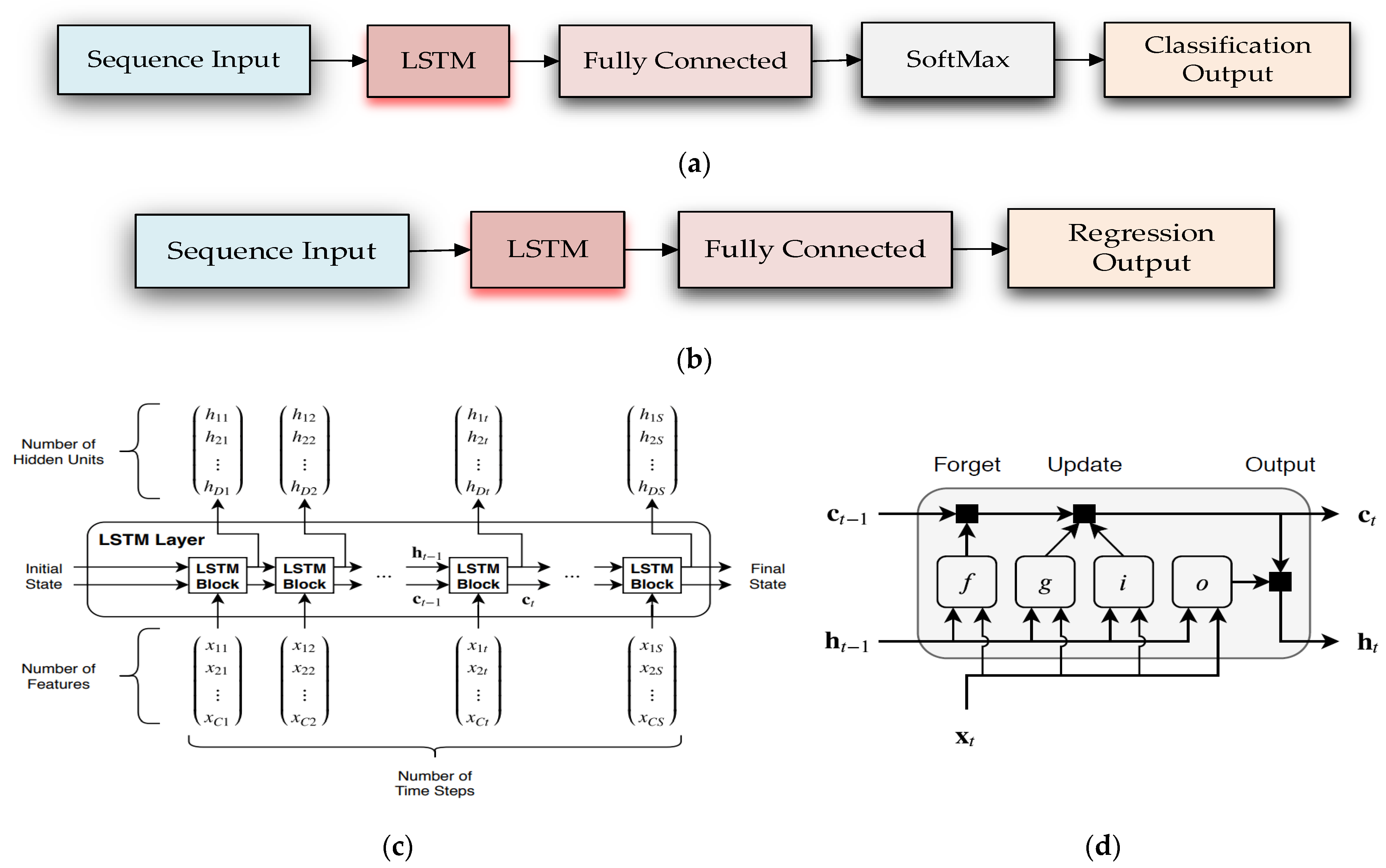
2.2.3. LSTM Li-Ion Battery SOC Estimation and Fault Detection using LSTM Deep Learning Neural Network

A long short-term memory (LSTM) neural network is a type of recurrent neural network (RNN) which is used to learn, process, and classify sequential data [39,40,41]. These networks can have the ability to learn long-term dependencies between time steps of input-output dataset measurements. An LSTM network processes input data by looping over time steps and updating the network state [39,40,41]. The network state contains information remembered over previous time steps. The LSTM is a Deep Learning Neural Network technique adapted in this research to detect the anomalies (faults) in Li-ion batteries, as a viable alternative to Joint EKF state and parameter estimation for Fault Detection and Diagnosis presented in Section 3.1. The LSTM is a data-based learning technique compared to EKF, a model-based estimation technique, and thus more suitable for online learning applications. Two of the LSTM neural network architectures are adapted to our case study that differs in the number of layers depending on the type of application if it is a classification or a regression. Two of these layers represent the core of the entire structure, namely a sequence input layer, and the second is an LSTM layer. The role of the sequence input layer is to input a sequence or time series data into the neural network, while the LSTM layer learns long-term dependencies between time steps of input sequence data [41]. Two simplified diagrams of an LSTM neural network (LSTMNN) and another two that illustrate a detailed LSTMNN architecture and the flow of data at current time t are presented in Figure 11, as shown in [41].
This diagram from Figure 11a shows an LSTM neural network architecture of classification type. It starts with a sequence input layer followed by an LSTM layer. To predict class labels, the LSTM layer is followed by three other layers connected in series: a fully connected layer, a SoftMax layer, and a classification output layer. Similarly, the second diagram from Figure 11b is a simplified LSTM neural network architecture obtained from the first diagram by removing the last two layers (SoftMax and Classification) and then replacing them with a Regression layer. The LSTM neural network architecture diagram shown in Figure 11c details the flow of a time series X with C features (channels) of length S through an LSTM layer. The first LSTM block uses the initial state of the RNN and the first-time step of the sequence to compute the first output and the updated cell state. At time step t, the first block of this diagram uses the current state of the RNN ( c t 1 , h t 1 ) and the next time step of the sequence to compute the output and the updated cell state c t . Thus, each layer of the diagram has its internal dynamics, described by the evolution of the cell state c t at time step t and of its output h t , known as the hidden state [41]. The hidden state at time step t contains the output of the LSTM layer for this time step. The cell state “contains information learned from the previous time steps” [41]. At each time step, the layer is updated by adding information to the cell state or resetting the content of the cell state by removing information from it. The layer controls these updates using gates. The following diagram shown in Figure 11d illustrates how a layer’s cell state is controlled by four components [41]:
  • Input gate (i) controls the level of cell state update
  • Forget gate (f) controls the level of cell state reset (forget)
  • Cell candidate (g) adds information to the cell state.
  • Output gate (o) controls the level of cell state added to the hidden state.
In the same, Figure 11d is explained how the gates forget, update, and output the cell and hidden states, using four blocks designated by i, f, g, and o to denote the input gate, forget gate, cell candidate, and output gate, respectively [41].
The overall dynamics of the cell and hidden states at time step t are described by following two equations [41]:
c t = f t c t 1 + i t g t
h t = o t σ c ( c t ) ,   σ c ( c t ) = 1 1 + e c t
where ⊙ symbolizes the Hadamard product, an element-wise multiplication operation of vectors, and σc designates the state activation function. The lstmLayer function uses, by default, the sigmoid function, i.e., a hyperbolic tangent function (tanh), to compute the state activation function, as in Equation (9).
The four blocks of the diagram shown in Figure 11d and denoted by i t as input gate, f t —forget gate, g t —cell candiadate, and o t output gate is described at step time t as a sigmoidal nonlinear activation function:
  • Input gate: i t = σ g ( W i x t + R i h t 1 + b i )
  • Forget gate: f t = σ g ( W f x t + R f h t 1 + b f )
  • Cell candidate: g t = σ c ( W g x t + R g h t 1 + b g )
  • Output gate: o t = σ g ( W o x t + R o h t 1 + b o )
where ( W i , W f , W g , W o ) , ( R i , R f , R c , R o ) and ( b i , b f , b g , b o ) represent the input weight matrices, recurrent weight matrices and bias vector that concatenate the input weights, the recurrent weights, and the bias of each component, respectively.
The LSTM neural network deep learning classification allows inputting sequence dataset input-output measurements into a network. It makes predictions based on the individual time steps of the sequence dataset. In the case study for the proposed Li-ion battery model that generates the healthy and faulty data measurements is trained an LSTM neural network deep learning (more than a hidden layer structure) is to recognize the combination (Vbat, SOC) of dataset measurements as time series data corresponding to health, voltage fault, current fault, and false alarm (misclassification) class (0, 1, 2 and 3). The training data contains time series data for the same LIB SOC and Terminal voltage adopted in the previous section. Each sequence has four features and doesn’t vary in length. The data set contains 2477 training observations and 2477 test observations.
The subsequent steps are followed to adapt the LSTM neural network deep learning classification of the health and anomalies detected classes in the faulty signals representing the Li-ion battery terminal voltage and its SOC, as suggested in [40]:
Step 1.
Load dataset input-output measurements (healthy-subscript h, faulty: subscript fv for voltage fault, fc for current fault, and for dataset test to asses the classification accuracy is used the subscript new)
Vbat = [Yh Yfv Yh_new Yfc] is battery terminal voltage sequence: healthy-voltage fault-new healthy dataset-current fault
SOC = [SOCh SOCfv SOC_new SOCfc] for the battery SOC sequence with the same meaning as for Vbat
Step 2.
Create Cell Array for XTrain and YTrain with combinations of Vbat and SOC,
Condition Code: 0-Healthy, 1-Fault Voltage,2-Fault Current; 3-False alarm.
XTrain = {[Yh,SOCh]’; [Yfv,SOCfv]’; [Yh_new,SOCh_new]’; [Yfc,SOCfc]’; [Yh,SOCfc]’} is training input sequence
YTrain = categorical{[‘0′,’1′,’2′,’3′]} denotes the output training sequence for anomaly classification (diagnosis)
Step 3.
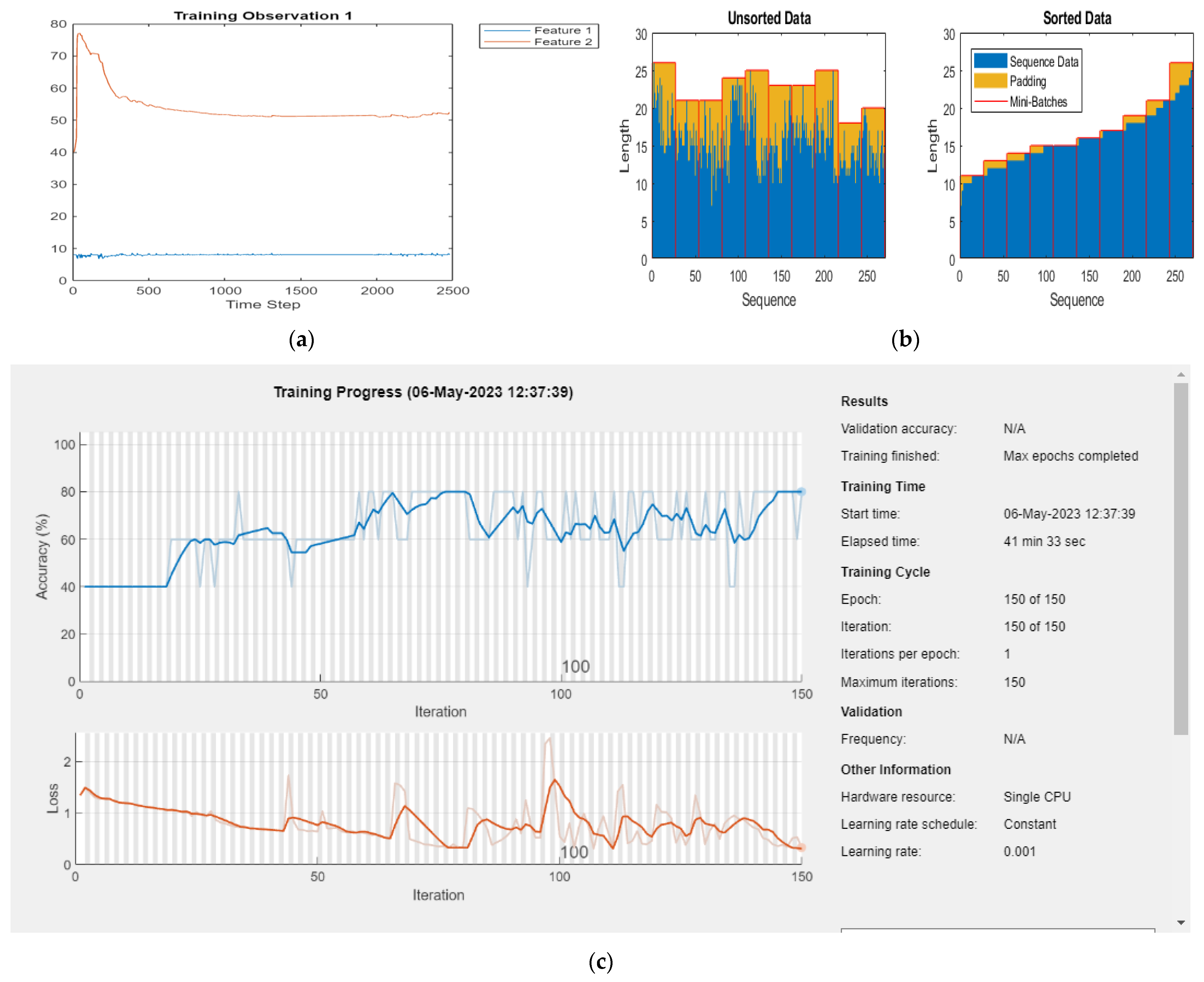
Visualize the first time series in a plot. Each line corresponds to a feature.
Step 4.
Prepare the dataset for padding: During training, by default, the software splits the training data into mini-batches and pads the sequences so that they have the same length. However, too much padding can have a negative impact on the network performance.
Remark 1.
In the case that the observations haven’t the same length, to prevent the training process from adding too much padding, the training data can be sorted by sequence length, and the hen has selected a mini-batch size so that sequences in a mini-batch have a similar length.
Step 5.
Choose a mini-batch size of 50 to divide the training data evenly and reduce the amount of padding in the mini-batches.
Step 6.
Define the LSTM neural network architecture:
Step 6.1.
Specify the input size to be sequences of size 2 (the dimension of the input data: 4 features, each of dimension 2 × 2477)).
Step 6.2.
Specify a bidirectional LSTM layer with 250 hidden units, and output to the “last” element of the sequence.
Step 6.3.
Specify four classes by including a fully connected layer of size 4 (number of features), followed by a SoftMax layer and the classification layer.
Step 6.4.
Specify the options:
Step 6.4.1.
Specify solver to be “adam”
Step 6.4.2.
Setup the gradient threshold to be 0.5
Step 6.4.3.
Setup the maximum number of epochs to be 150.
Step 6.4.4.
Specify the sequence length to be “longest” (for the same length)
Step 7.
LSTM Training data phase
net = trainNetwork (XTrain, YTrainn, Layers, options)
Step 8.
LSTM data Test: test the LSTM with a never seen data input sequence.
XTest = {[Yh, SOCh_new]’}
YTest = categorical {[‘0′]}
Step 9.
LSTM Classification of the test data:
YPred = classify (net, XTest), …
MinibatchSize = minibatchSize,
SequenceLength = “longest”
Step 10.
Calculate the classification accuracy of the predictions:
acc = sum (YPred==YTest/numel (YTest))
The value of the LSTM neural network classification accuracy is the highest number 1; thus, the LSTM has excellent classification accuracy. Also, for a new combination, with an input never seen, the result is correct with an accuracy of 1.
  • XTestnew = [Yh_new, SOCh]’;
  • YPred = classify (net, XTest1)’,…
  • MiniBatchSize =miniBatchSize,…
  • SequenceLength = (“longest”);
  • acc = sum (YPred –Ytest/numel (Ytest)
  • YPred = 0;
  • acc = 1;

3. Results

3.1. Li-Ion Cobalt Battery Type -Statistics Performance Evaluation

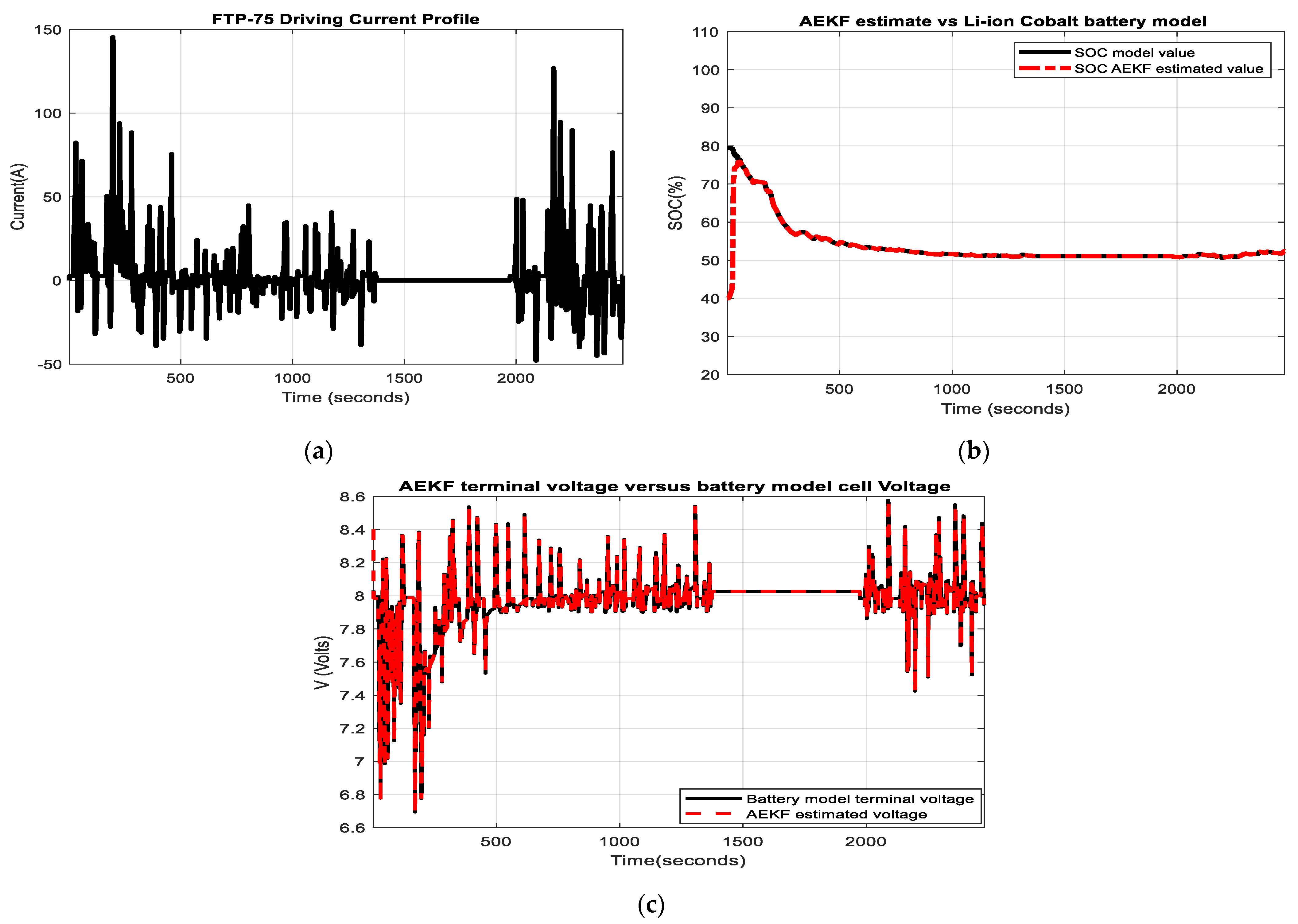
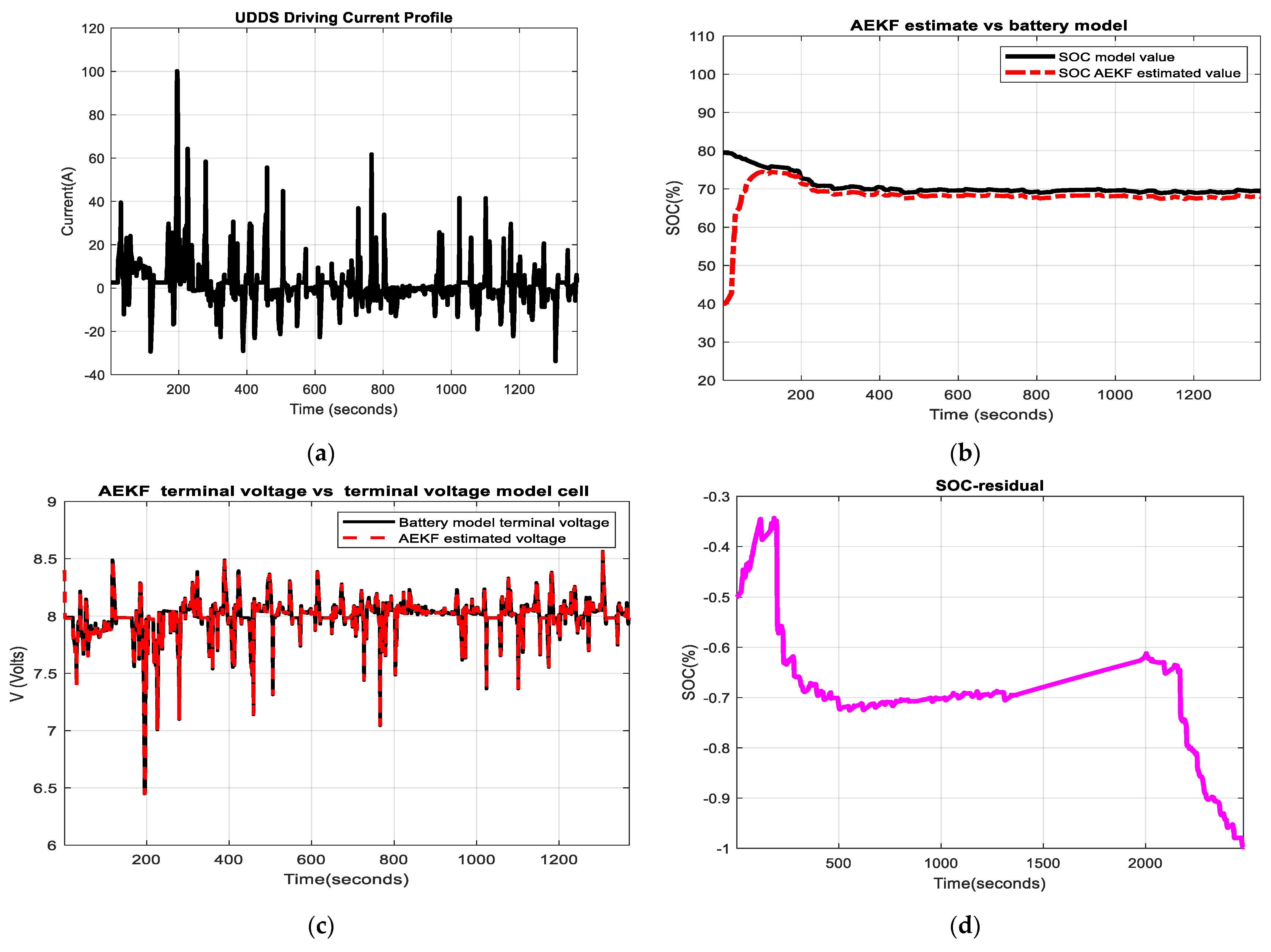
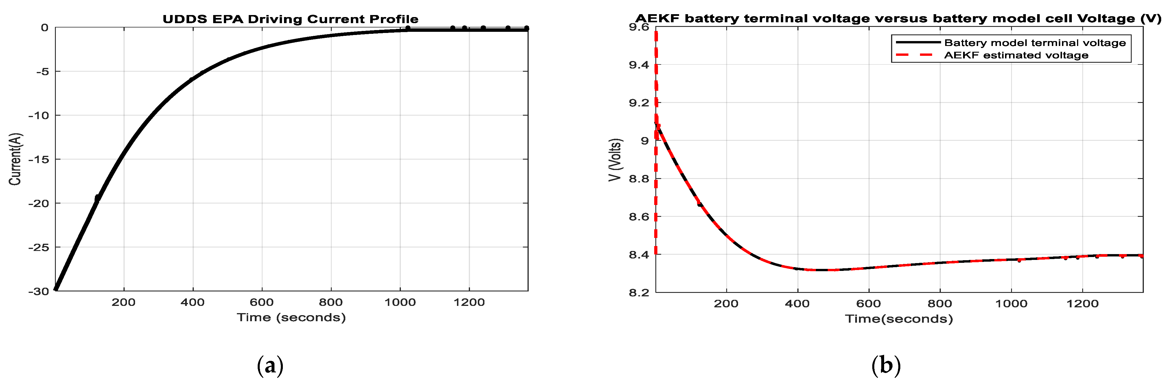
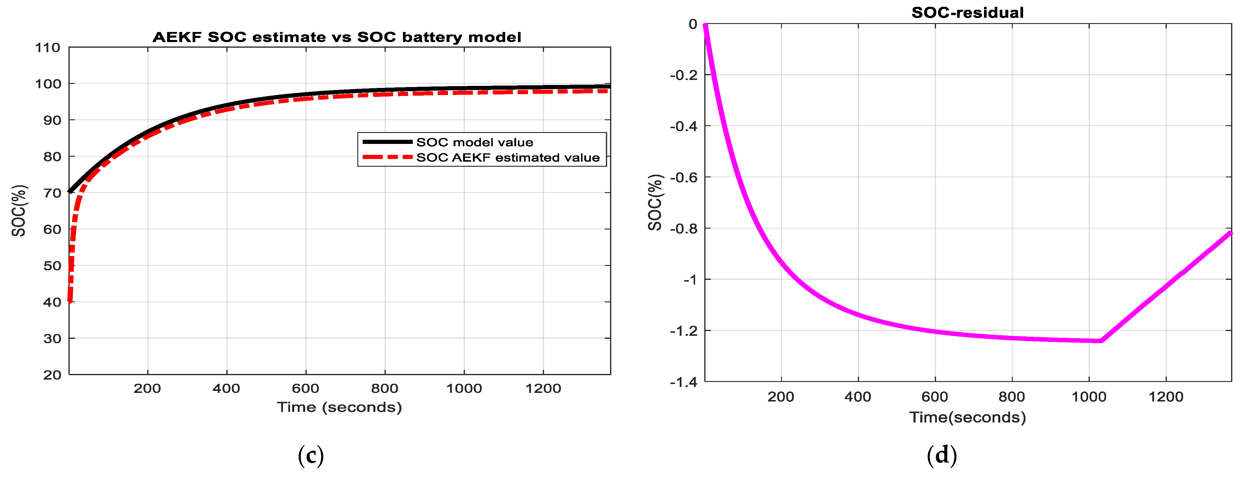
Li-Ion Cobalt Battery Generic Model- AEKF SOC Estimator Simulation Results

To analyze the SOC accuracy performance of the generic Simulink Simscape battery model and to prove its robustness to changes in the initial SOC values from 80% to 40%, noise level and different driving cycle current test profiles, such as FTP-75, UDDS and UDDS-EPA, a comparison of the battery performance in terms of the AEKF SOC cell estimates and battery terminal voltage versus the true battery cell values is performed in the Figure 12a–c, and in Figure 13a–d and Figure 14a–d which are showing also the SOC residuals. The EKF SOC estimator algorithm steps are the same as those presented briefly in [22,23,24], and Annex A of [37].
In the last three Figure 12, Figure 13 and Figure 14, the MATLAB simulation results reveal the same robustness of the AEKF SOC estimator to changes in the initial SOC value starting from 40% battery charged instead of 80% as in the battery model and to switching the driving style from one profile to another, namely FTP-75, UDDS and EPA that are the most used driving cycle tests.
The accuracy performance of the battery SOC is evaluated by using statistic performance criteria capable of justifying the Li-ion battery model selection. In the case study are preferred the root mean square error (RMSE), mean square error (MSE), mean absolute error (MAE) and standard deviation (Std), well defined and documented in [11]. As a baseline for the battery SOC model, errors are the estimated value of SOC by the AEKF algorithm at SOC initial value = 80%. The results are shown in Table 1.
The MATLAB simulation results presented in all Figure 12, Figure 13 and Figure 14 reveal an excellent SOC accuracy performance for the adopted Li-ion battery model, valuable information extracted from the residual value of SOC which is smaller than 1% compared to the 2% reported in the literature. Also, the statistical criteria used for SOC accuracy evaluation confirm the same excellent accuracy of the AEKF SOC estimate compared to the actual value of the battery model.

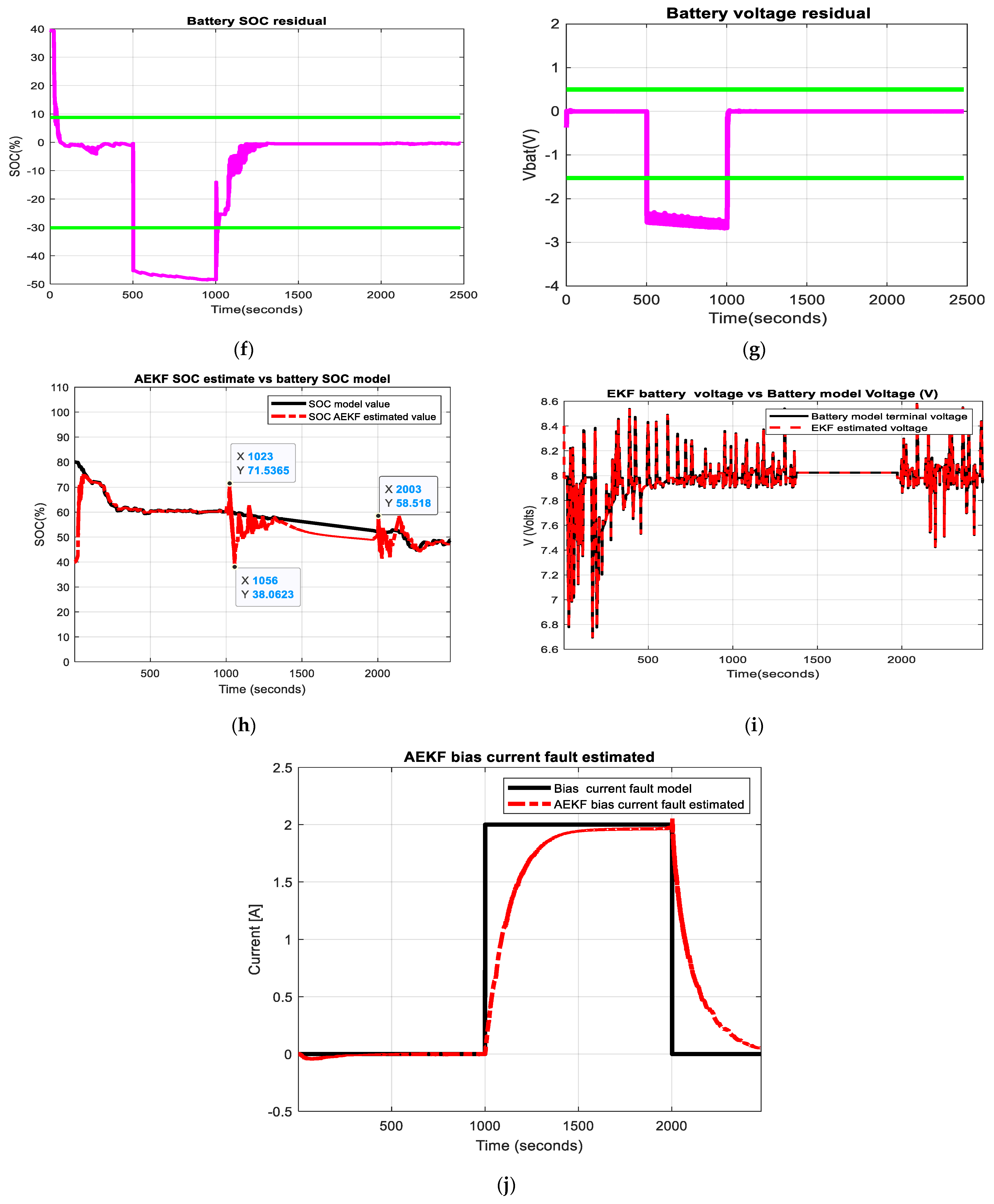
3.2. MATLAB Simulation Results for Joint Parameter and State Estimation EKF for Fault Detection and Isolation

The MATLAB simulation results for JEKF are depictured in Figure 15a–l. Figure 15a,b are shown the AEKF Rint and temperature estimates versus LIB model values. In Figure 15c is depicted the AEKF LIB SOC. In Figure 15d is illustrated the terminal voltage, in Figure 15e you can see the voltage fault estimates values, and in Figure 15f is visualized the residual of battery SOC; the terminal voltage of LIB model for voltage fault is shown in Figure 15g. The last set of Figure 15h–l have the same signification as for the faulty current LIB model.
The thresholds for Bias Voltage fault ( f V ) and Current fault ( f I ) are calculated as follows [35]:
S O C t h r e s h o l d = m e a n ( S O C r e s i d u a l )   3 s t d ( S O C r e s i d u a l )
V b a t t t h r e s h o l d = m e a n ( V b a t r e s i d u a l )   3 s t d ( V b a t r e s i d u a l )
where mean and std denote the average and standard deviation statistics.
The performance analysis of AEKF SOC, Terminal voltage and both ( f V ,   f I ) bias faults estimates are done by comparison of each residual of LIB SOC and terminal voltage, as a difference between measurements and estimates, collected from three parallel AEKF filters bank, one to simulate the health condition (code 0), voltage faulty condition (code 1), and current faulty condition (code 2) of three LIB models.
In Figure 15f,g represented the SOC and terminal voltage residuals for the faulty LIB model obtained by injecting in Equation (7) an addition bias voltage fault ( f V ) of 3V magnitude (Figure 15d), and in the Equations (3), (4) and (6) an addition bias current ( f I ) of 2A magnitude (Figure 15i). The detection of the faults is occurred very close to the injection instant (500 s and 1000 s respectively, and the voltage fault is removed fast, after 700 s, at the end of the window [500,1200] (seconds) in contrast to the current-voltage which is removed after a delay of approx. 400 s after the end of the injection window [1000,2000] (seconds) as is shown in Figure 15i. For the diagnosis of both faults (anomalies) is used, the following signature matrix is shown in Table 2.
In this Table, the fM denotes a situation that could be met in realistic situations, namely a misclassified fault. The MATLAB simulation results reveal a very accurate estimation and robustness of the traditional EKF SOC estimator and terminal voltage predictor for changes in operating conditions and SOC initial values.

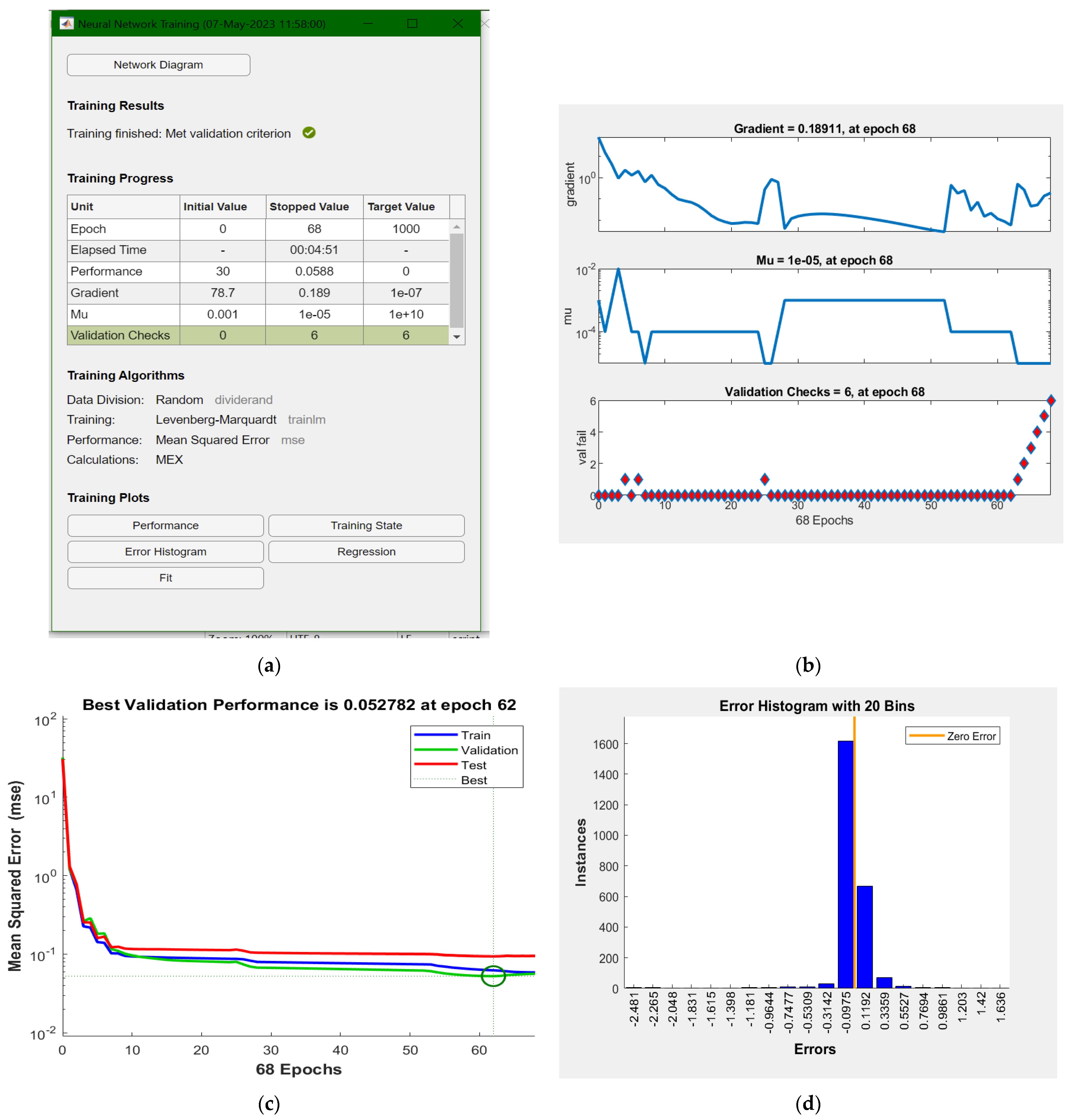
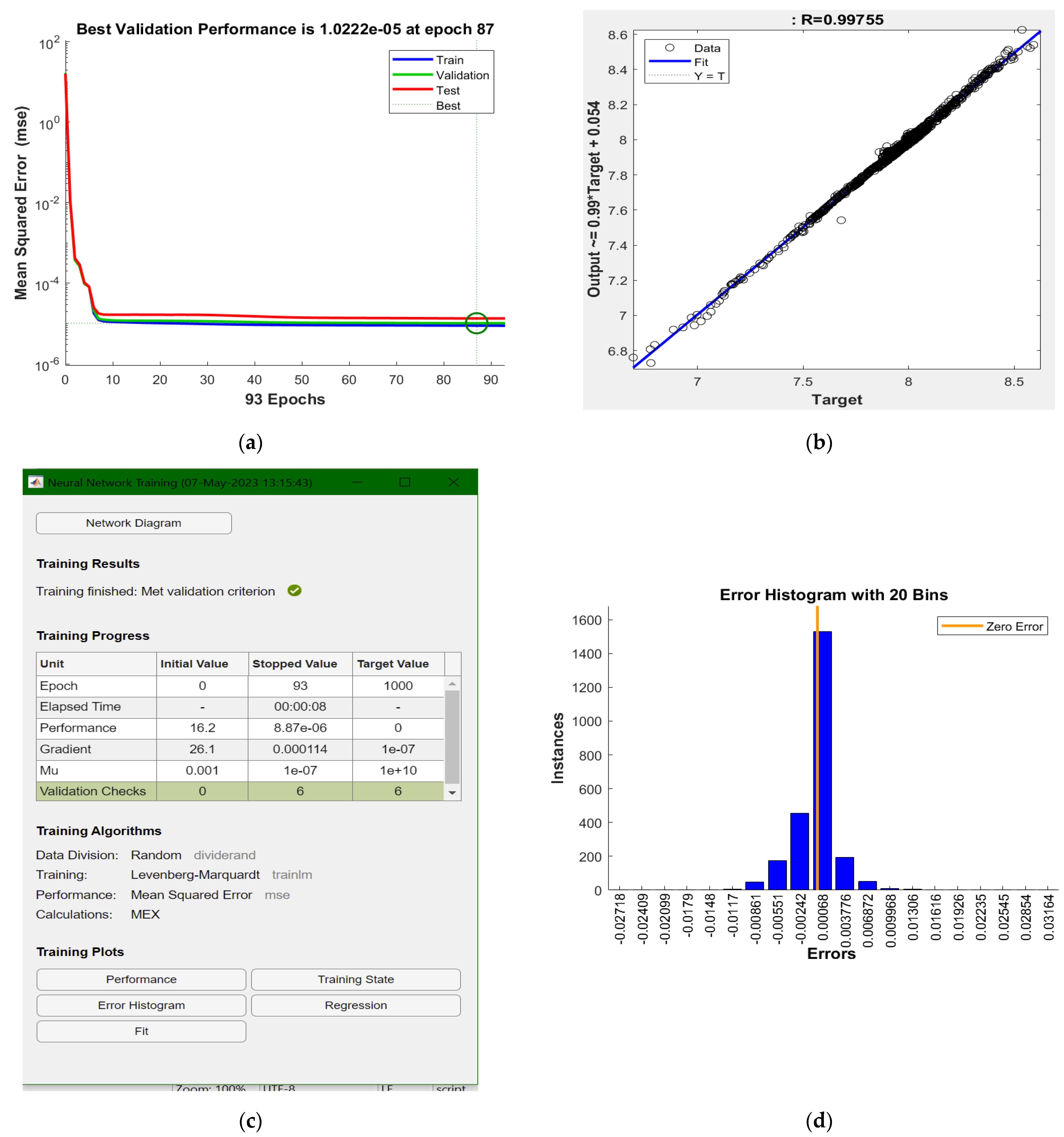
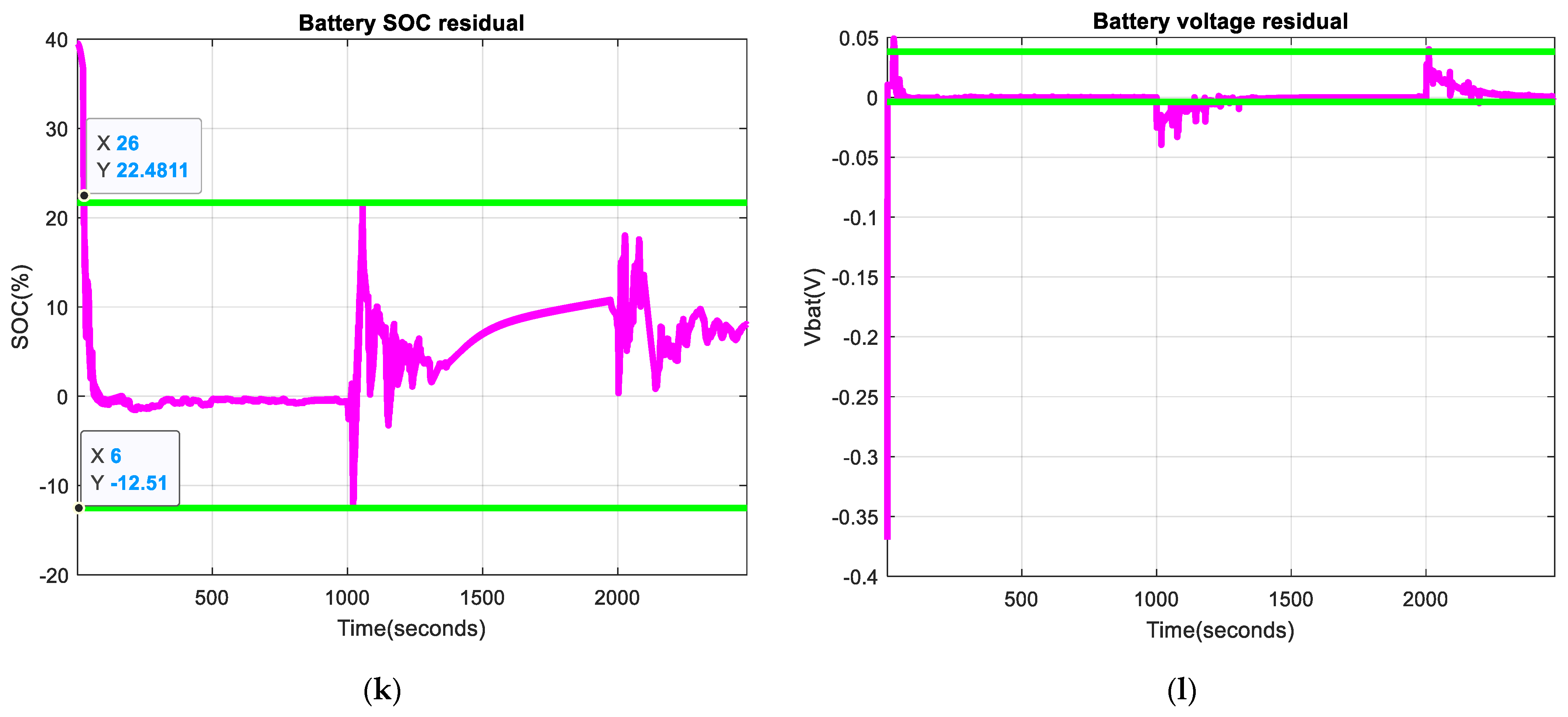
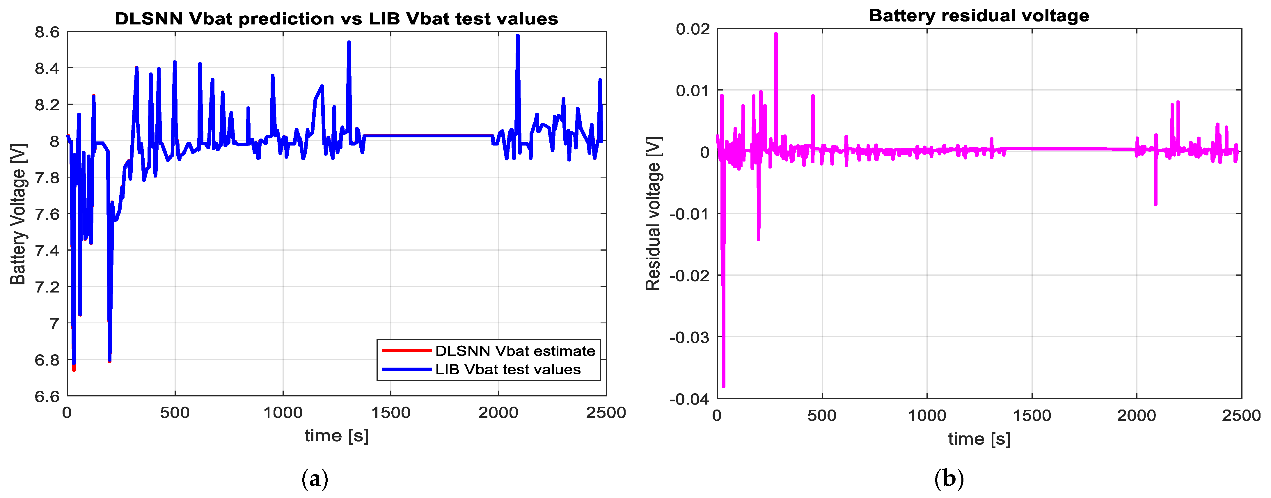
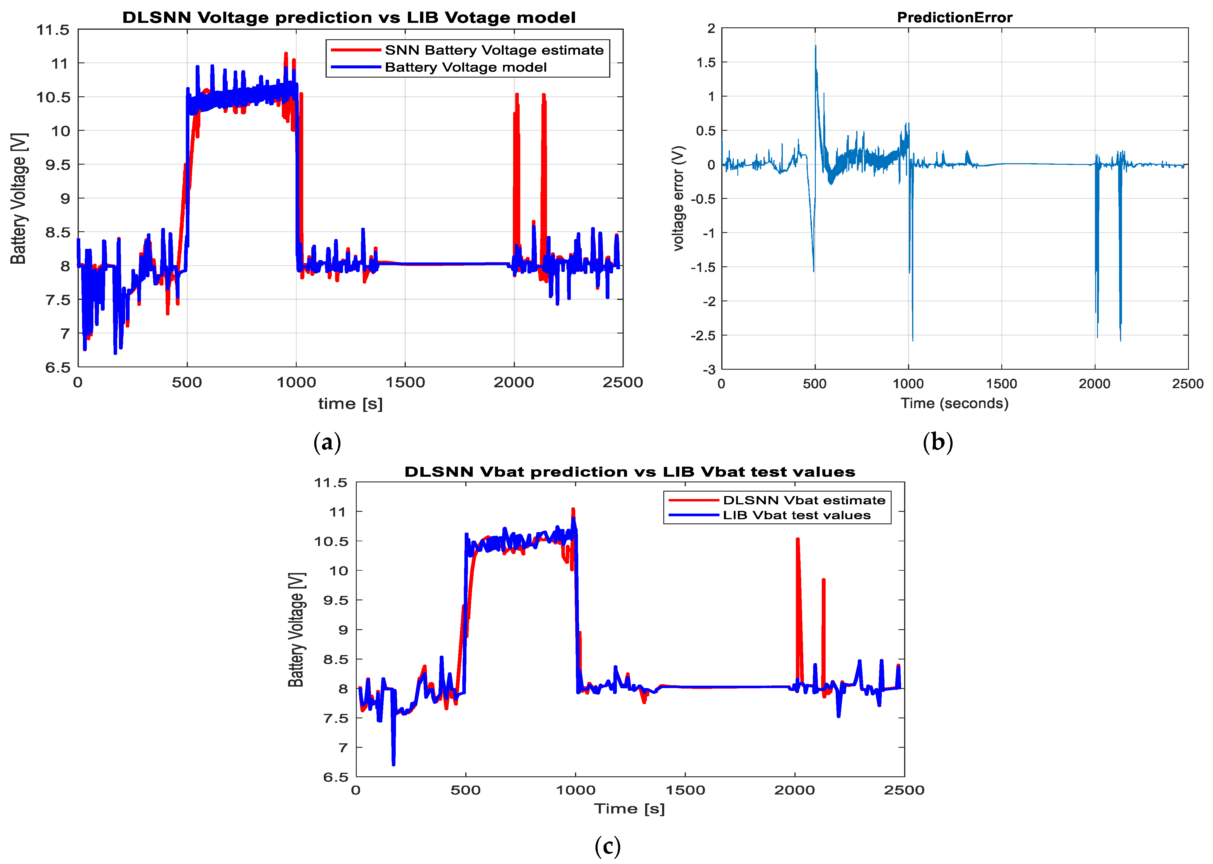
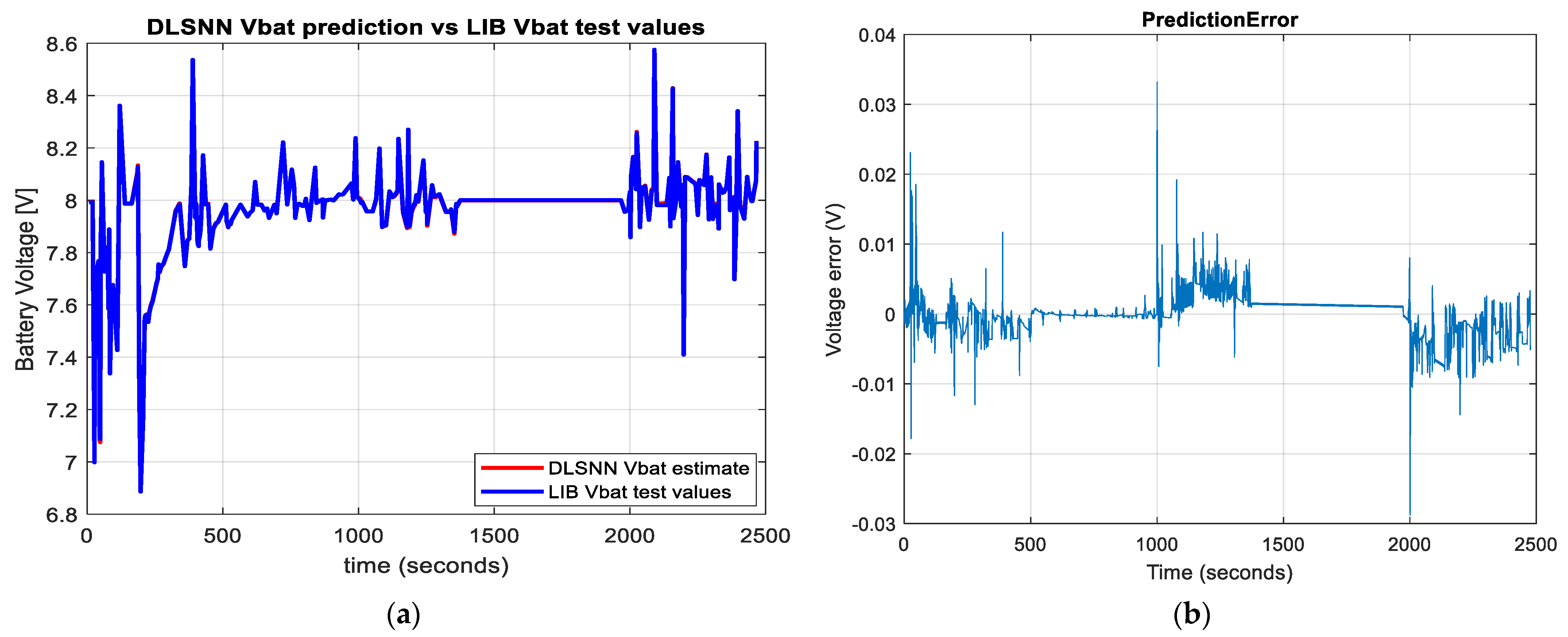
3.3. DLSNN MATLAB Simulation Results

For the healthy scenario, Figure 16a,b illustrates the DLSNN prediction performance for the terminal voltage of LIB Vbat in Figure 16a. For performance assessment is depicted in Figure 16b, the LIB voltage residual.
Returning to Figure 8e, it can be noted an excellent 8.15 × 10 7 mse overall performance for the adopted DLSNN, thus slightly superior compared to the traditional EKF SOC estimation and Voltage prediction algorithm employed in the previous subsection.
For faulty voltage scenarios, the MATLAB simulation results are presented in Figure 17a–c. In addition, Figure 17a illustrates the DLSNN Voltage fault prediction, Figure 17b shows the DLSNN prediction voltage error, and Figure 17c reveals DLSNN’s performance for the data set test.
For faulty current scenarios, the MATLAB simulation results are depicted in Figure 18a for showing the DLSNN prediction voltage, and 18b to assess the DLSNN prediction voltage error. For all three scenarios, the outstanding prediction performance of DLSNN shows performance superiority compared to the EKF estimator. However, due to the voltage anomaly in the measurement dataset, the mse performance of 0.0469 is lower compared to the mse performance for healthy LIB that reaches.
The impact of the current anomaly in the measurement dataset on mse performance is comparable to those met for healthy LIB, namely of 8.31 × 10 5 , better than the second scenario of anomaly detected in the Voltage sensor dataset. In conclusion, the main advantage of using the DLSNN technique lies in its data-driven feature and excellent accuracy performance; thus, is not required the battery model, which in almost all realistic cases is affected by uncertainties and unmodeled parts; the accuracy of the DLSNN prediction is only affected by the quality of the data set.

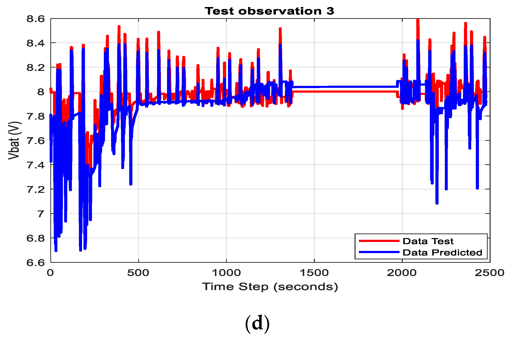
3.4. The LSTM Anomaly Classification-MATLAB Simulation Results

The training phase, the first observation and the padding task are illustrated in Figure 19a–c.
The accuracy performance of the LSTM deep learning neural network to classify the four classes reaches 80%, and the loss is very small, around 0.2. Thus it performs very well, and it can correctly classify a combination (SOC, Vbat) never seen, with an accuracy equal to 1.
In this research work, we investigate further the regression ability of the LSTM to predict the values of variables SOC and Vbat combined in the same sequence (health-voltage fault-health-current fault) tested for classification. Thus, the target (response) from the last output layer of the LSTM NN structure is now in numerical format, no more in cathegorical format as for classification events. The LSTM deep learning NN structure has only four blocks, as is exposed in Figure 11b. The last layer replaces the SoftMax layer from Figure 11a with a Regression layer. Readers can refer to [42,43] for details on this structure. The MATLAB simulation result is illustrated in Figure 20a–d for training phase progress and battery voltage prediction. Comparing the results of the MATLAB simulations shown in all three Figure 16, Figure 17 and Figure 18 for the DLSNN prediction technique to those shown in Figure 20a–d for LSTM, it is evident that the RMSE accuracy performance of LSTM Deep Learning NN with regression layer is lower. Thus DLSNN prediction technique performs better. The LSTM parameters must be returned by “trial and error” until the performance is comparable to DLSNN or unsuitable for this application. Therefore, our focus remains on the DLSNN regression network, and future work will be under new investigations.

4. Discussion

Achieving the main objective of this paper requires a lot of documentation effort. Rigorous documentation involves time, passion, respect, and responsibility for the reader thirsty for knowledge and creativity. The information gathered during documentation and then disseminated to the reader must be of high quality, scientifically valuable, innovative and of genuine interest to him from a theoretical and practical point of view. Indeed, strict adherence to the fulfilment of these requirements combined with the editorial ones is the key to the success, validation, and recognition of the value of the complete research results.
Furthermore, the complexity of this research work was an ample opportunity for us to enhance our experience in control systems significantly. Among them, the processes of identification, modelling, state estimation, and supervised and unsupervised neural networks, each of one or combined, open exciting research directions. Additionally, getting good skills in algorithmic and systemic approaches helps develop, program and real-time implementation of Li-ion battery SOC estimators and terminal voltage predictors on the MATLAB Simulink software platform. For “proof concept” and simulations purposes is adopted a Simulink Simscape generic model of a preset Li-ion Cobalt of 5.4 Ah rated capacity and 7.2 V nominal voltage that could be integrated into a BMS for possible usage in an extensive palette of HEVs and EVs applications with promising future potential in the automotive industry. The proposed Li-ion Cobalt battery parameter values are extracted from a specific Simulink Simscape block setup of a preset Li-ion Cobalt battery tested using an FTP-75 discharge driving cycle profile. The accuracy performance of the SOC model is excellent, with an error of less than 0.5% at steady state, compared to the 2% error reported in the literature. An accurate Li-ion battery model has a significant impact on the accuracy of the EKF estimator, revealed by MATLAB simulation results that indicate high SOC accuracy and robustness to changes in the initial SOC estimate from 80% to 30% and 40% and also to changes in driving cycles from FTP-75 to the most widely used UDDS and EPA UDDS tests. A bank of three EKF SOC estimators and terminal voltage predictors generates the SOC and Voltage residuals for three scenarios: healthy, bias voltage and bias current faults in the measurement sensors. Thus, an FDI technique residual based on a traditional EKF FDI strategy can detect all three scenarios and diagnose the type of each fault. As a valuable alternative to the conventional EKF FDI strategy model based, in this research are made several investigations to adapt advanced intelligent data-driven methods to generate all fault scenarios, namely a DLSNN learning model of high accuracy, assessed by RMSE performance of 0.0588 (for Voltage fault) and around 5.5 × 10 7 (healthy) and 8.87 × 10 6 (current fault) slightly superior compared to the traditional EKF FDI strategy, RMSE around 0.007.

5. Conclusions

This research combines traditional and advanced AI-inspired intelligent approaches from machine learning (ML) and deep learning (DL) models. The proposed Li-ion Cobalt battery is a generic Simulink Simscape model. Therefore, the battery parameter values are extracted from the Simulink Simscape battery block setup for a preset Li-ion Cobalt battery tested for three driving cycles: an FTP-75, USSD and EPA USSD. The LSTM deep learning neural network technique used in this work proved valuable for anomaly detection and diagnosis by classification with high accuracy, around 80%, and a loss performance very close to zero. Furthermore, we have also investigated the use of LSTM DLNN to generate the same scenarios by using the regression feature of its structure. However, the MATLAB simulation result reveals a lower regression RMSE performance accuracy for all three scenarios than the DLSNN regression learning model. In future work, we will continue our investigations on improving LSTM performance for the regression of data time series.

Author Contributions

R.-E.T. has contributed to algorithms conceptualization, manuscript preparation, and writing. N.T. has contributed to battery model validation, performed MATLAB simulations, and analyzed the results. M.S.R. and M.Z. have contributed a formal analysis of the results for the visualization, project supervision and administration. Finally, H.C. contributed to manuscript preparation, corrections, visualization, and formal analysis. All authors have read and agreed to the published version of the manuscript.

Funding

This research received no external funding.

Data Availability Statement

Not applicable.

Conflicts of Interest

The authors declare no conflict of interest.

References

  1. Becker, P.D. Alternative Energy; Christine Nasso, Greenhaven Press: Farmington Hills, MI, USA, 2010; 132p. [Google Scholar]
  2. García-Olivares, A.; Solé, J.; Osychenko, O. Transportation in a 100% renewable energy system. Energy Convers. Manag. 2018, 158, 266–285. [Google Scholar] [CrossRef]
  3. Young, K.; Wang, C.; Wang, L.Y.; Strunz, K. Electric vehicle battery technologies. In Electric Vehicle Integration into Modern Power Networks, 1st ed.; Garcia-Valle, R., Jap, L., Eds.; Springer: New York, NY, USA, 2013; Chapter 2; pp. 15–26. [Google Scholar] [CrossRef]
  4. Conserve Energy Future. Available online: https://www.conserve-energy-future.com/advantages-and-disadvantages-of-electric-cars.php (accessed on 19 November 2022).
  5. Gao, Z.; Chin, C.S.; Chiew, J.H.K.; Jia, J.; Zhang, C. Design and Implementation of a Smart Lithium-Ion Battery System with Real-Time Fault Diagnosis Capability for Electric Vehicles. Energies 2017, 10, 1503. [Google Scholar] [CrossRef]
  6. Hu, X.; Zhang, K.; Liu, K.; Lin, X.; Dey, S.; Onori, S. Advanced Fault Diagnosis for Lithium-Ion Battery Systems. TechRxiv 2020, preprint. [Google Scholar] [CrossRef]
  7. Xia, B.; Zheng, W.; Zhang, R.; Lao, Z.; Sun, Z. A Novel Observer for Lithium-Ion Battery State of Charge Estimation in Electric Vehicles Based on a Second-Order Equivalent Circuit Model. Energies 2017, 10, 1150. [Google Scholar] [CrossRef]
  8. Zhang, X.; Wang, Y.; Wu, J.; Chen, Z. A novel method for lithium-ion battery state of energy and state of power estimation based on multi-time-scale filter. Appl. Energy 2018, 216, 452–461. [Google Scholar] [CrossRef]
  9. Luo, L.; Zhang, C.; Tian, Y.; Liu, H. State-of-Health Estimate for the Lithium-Ion Battery Based on Constant Voltage Current Entropy and Charging Duration. World Electr. Veh. J. 2022, 13, 148. [Google Scholar] [CrossRef]
  10. Tudoroiu, R.-E.; Zaheeruddin, M.; Tudoroiu, N.; Radu, S.-M. SOC Estimation of a Rechargeable Li-Ion Battery Used in Fuel-Cell Hybrid Electric Vehicles—Comparative Study of Accuracy and Robustness Performance Based on Statistical Criteria. Part I: Equivalent Models. Batteries 2020, 6, 42. [Google Scholar] [CrossRef]
  11. Tudoroiu, N.; Zaheeruddin, M.; Tudoroiu, R.-E. Real Time Design and Implementation of State of Charge Estimators for a Rechargeable Li-ion Cobalt Battery with Applicability in HEVs/EVs-A comparative Study. Energies 2020, 13, 2749. [Google Scholar] [CrossRef]
  12. Sensata Technologies. Lithium Balance Battery Management Systems. Available online: https://lithiumbalance.com/applications (accessed on 19 November 2022).
  13. Alvarez, J.M.; Sachenbacher, M.; Ostermeier, D.; Stadlbauer, H.J.; Hummitzsch, U.; Alexeev, A. Analysis of the State of the Art on BMS; Everlasting D6.1 Report; Lion Smart GmbH: Munchen, Germany, 2017. [Google Scholar]
  14. Roderick, R. A Look inside Battery-Management Systems Electronic Design. 2015. Available online: http://electronicdesign.com/power/look-inside-battery-management-systems (accessed on 20 November 2022).
  15. Jung, S.; Jeong, H. Extended Kalman Filter-Based State of Charge and State of Power Estimation Algorithm for Unmanned Aerial Vehicle Li-Po Battery Packs. Energies 2017, 10, 1237. [Google Scholar] [CrossRef]
  16. Liu, G.; Zhang, L. Research on the Thermal Characteristics of an 18650 Lithium-Ion Battery Based on an Electrochemical–Thermal Flow Coupling Model. World Electr. Veh. J. 2021, 12, 250. [Google Scholar] [CrossRef]
  17. Zhao, Y.; Zou, B.; Li, C.; Ding, Y. Active cooling-based battery thermal management using composite phase materials. In Proceedings of the 10th International Conference on Applied Energy (ICAE2018), Hong Kong, China, 22–25 August 2018; Volume 158, pp. 4933–4940. [Google Scholar] [CrossRef]
  18. Huria, T.; Ceraolo, M.; Gazzarri, J.; Jackey, R. High Fidelity Electrical Model with Thermal Dependence for Characterization and Simulation of High-Power Lithium Battery Cells. In Proceedings of the IEEE International Electric Vehicle Conference, Greenville, SC, USA, 8 April 2012. [Google Scholar] [CrossRef]
  19. Baronti, F.; Fantechi, G.; Fanucci, L.; Leonardi, E.; Roncella, R.; Saletti, R.; Saponara, S. State-of-Charge Estimation Enhancing of Lithium batteries through a Temperature–Dependent Cell Model. In Proceedings of the 2011 International Conference on Applied Electronics, Pilsen, Czech Republic, 7–8 September 2011; pp. 1–5. [Google Scholar]
  20. Nugroho, A.; Rijanto, E.; Wijaya, F.D.; Nugroho, P. Battery state of charge estimation by using a combination of Coulomb Counting and dynamic model with adjusted gain. In Proceedings of the 2015 International Conference on Sustainable Energy Engineering and Application (ICSEEA), Bandung, Indonesia, 5–7 October 2015; pp. 54–58. [Google Scholar] [CrossRef]
  21. Yuan, S.; Wu, H.; Yin, C. State of Charge Estimation Using the Extended Kalman Filter for Battery Management Systems Based on the ARX Battery Model. Energies 2013, 6, 444–470. [Google Scholar] [CrossRef]
  22. Plett, G.L. Extended Kalman filtering for battery management systems of LiPB-based HEV battery packs: Part 1. Background. J. Power Sources 2004, 134, 252–261. [Google Scholar] [CrossRef]
  23. Plett, G.L. Extended Kalman filtering for battery management systems of LiPB-based HEV battery packs: Part 2. Modeling and identification. J. Power Sources 2004, 134, 262–276. [Google Scholar] [CrossRef]
  24. Plett, G.L. Extended Kalman filtering for battery management systems of LiPB-based HEV battery packs: Part 3. State and parameter estimation. J. Power Sources 2004, 134, 277–292. [Google Scholar] [CrossRef]
  25. Julier, S.J.; Uhlmann, J.K. A New Extension of the Kalman Filter to Nonlinear Systems. In Proceedings of the 11th International Symposium on Aerospace/Defence Sensing, Simulation and Controls, Orlando, FL, USA, 21–25 April 1997. [Google Scholar]
  26. Van der Merwe, R.; Wan, E.A. The square-root unscented Kalman filter for state and parameter-estimation. In Proceedings of the 2001 IEEE International Conference on Acoustics, Speech, and Signal Processing, Salt Lake City, UT, USA, 7–11 May 2001. [Google Scholar] [CrossRef]
  27. Jiani, D.; Youyi, W.; Changyun, W. Li-ion battery SOC estimation using particle filter based on an equivalent circuit model. In Proceedings of the 2013 10th IEEE International Conference on Control and Automation (ICCA), Hangzhou, China, 12–14 June 2013; pp. 580–585. [Google Scholar] [CrossRef]
  28. Aung, H.; Low, K.-S.; Soon, J.J. State-of-Charge Estimation Using Particle Swarm Optimization with Inverse Barrier Constraint in a Nanosatellite. In Proceedings of the 2015 IEEE 10th Conference on Industrial Electronics and Applications (ICIEA), Auckland, New Zealand, 15–17 June 2015; pp. 1–6. [Google Scholar] [CrossRef]
  29. Wu, T.; Wang, M.; Xiao, Q.; Wang, X. The SOC Estimation of Power Li-Ion Battery Based on ANFIS Model. Smart Grid Renew. Energy 2012, 3, 51–55. [Google Scholar] [CrossRef]
  30. Tudoroiu, R.-E.; Zaheeruddin, M.; Tudoroiu, N.; Radu, S.M. Smart Mobility—Recent Advances, New Perspectives and Applications; Sarwat, A., Khalid, A., Jalal, A.H., Eds.; Intech: Vienna, Austria, 2022; pp. 1–31. [Google Scholar] [CrossRef]
  31. Álvarez Antón, J.C.; García Nieto, P.J.; Blanco Viejo, C.; Vilán, J.A. Support Vector Machines Used to Estimate the Battery State of Charge. IEEE Trans. Power Electron. 2013, 28, 5919–5926. [Google Scholar] [CrossRef]
  32. Tudoroiu, N.; Zaheeruddin, M.; Tudoroiu, R.-E.; Radu, S.M. Wavelet Theory; Somayeh Mohammady; Intech: Vienna, Austria, 2020; pp. 1–37. [Google Scholar] [CrossRef]
  33. Hu, X.; Zhang, K.; Liu, K.; Lin, X.; Dey, S.; Onori, S. Advanced Fault Diagnosis for Lithium-Ion Battery Systems: A Review of Fault Mechanisms, Fault Features, and Diagnosis Procedures. IEEE Ind. Electron. Mag. 2020, 14, 65–91. [Google Scholar] [CrossRef]
  34. Dey, S.; Mohon, S.; Pisu, P.; Ayalew, B. Sensor Fault Detection, Isolation, and Estimation in Lithium-Ion Batteries. IEEE Trans. Control Syst. Technol. 2016, 24, 2141–2149. [Google Scholar] [CrossRef]
  35. MathWorks Documentation. Fault Detection Using a Kalman Filter. 2023. Available online: https://www.mathworks.com/help/predmaint/ug/Fault-Detection-Using-an-Extended-Kalman-Filter.html (accessed on 28 April 2023).
  36. MathWorks MATLAB Version R2023a Online Documentation. Fit Data with a Shallow Neural Network. Available online: https://www.mathworks.com/help/deeplearning/gs/fit-data-with-a-neural-network.html (accessed on 29 March 2023).
  37. Tudoroiu, N.; Zaheeruddin, M.; Tudoroiu, R.-E.; Radu, M.S.; Chammas, H. Intelligent Deep Learning Estimators of a Lithium-Ion Battery State of Charge Design and MATLAB Implementation—A Case Study. Vehicles 2023, 5, 535–564. [Google Scholar] [CrossRef]
  38. MathWorks Documentation. Identify Condition Indicators for Predictive Maintenance Algorithm Design. 2023. Available online: https://www.mathworks.com/help/predmaint/gs/identify-condition-indicators-for-predictive-maintenance-algorithm-design.html (accessed on 28 April 2023).
  39. MathWorks Documentation. Long-Short Term Memory (LSTM). 2023. Available online: https://www.mathworks.com/discovery/lstm.html (accessed on 30 April 2023).
  40. MathWorks Documentation. Sequence Classification Using Deep Learning. Available online: https://www.mathworks.com/help/deeplearning/ug/classify-sequence-data-using-lstm-networks.html (accessed on 1 May 2023).
  41. MathWorks Documentation. Long Short-Term Memory Neural Networks. 2023. Available online: https://www.mathworks.com/help/deeplearning/ug/long-short-term-memory-networks.html (accessed on 1 May 2023).
  42. MathWorks Documentation. Sequence-to-one Regression Using Deep Learning. 2023. Available online: https://www.mathworks.com/help/deeplearning/ug/sequence-to-one-regression-using-deep-learning.html (accessed on 4 May 2023).
  43. MathWorks Documentation. Sequence-to-sequence regression Using Deep Learning. 2023. Available online: https://www.mathworks.com/help/deeplearning/ug/sequence-to-sequence-regression-using-deep-learning.html (accessed on 4 May 2023).
Figure 1. The overall system architecture of a smart LIB power system (LCD: liquid-crystal display, SOC: state-of-charge, CAN BUS: controller area network bus, UART: universal asynchronous receiver-transmitter (reproduced from [5]).
Inventions 08 00074 g001
Figure 2. The BMS architecture with the main functional blocks (reproduced from [14]).
Inventions 08 00074 g002
Figure 3. The LiCoO2 Battery Simulink Simscape block setup for a preset Li-Ion battery generic 5.4 Ah rated capacity and 7.4 V nominal voltage without Temperature effects [11].
Inventions 08 00074 g003
Figure 4. Li-ion Battery model parameters and voltage discharging curves for different CC discharging current rates: (a) Nominal current discharge characteristic at 1.1 A; (b) The battery parameters and three current discharge characteristics.
Inventions 08 00074 g004
Figure 5. Parameters (a), Discharging current rates (b) and Temperature effects (c) for a generic Simscape LiCoO2 battery model.
Inventions 08 00074 g005aInventions 08 00074 g005b
Figure 6. MATLAB Simulink simulations results: (a) OCV-SOC battery curve; (b) the output voltages of both batteries; (c) the charging and discharging batteries constant currents; (d) the batteries SOCs; (e) ambient and cell temperatures in degrees Celsius.
Inventions 08 00074 g006aInventions 08 00074 g006b
Figure 7. Simulink Simscape model of Li-ion model for an FTP-75 driving cycle input current test profile (Notation: eta = η) (see [10]).
Inventions 08 00074 g007
Figure 8. Deep Learning Shallow Neural Network: (a) DL SNN structure; (b) Training phase; (c) Output Regression; (d) Error Histogram, (e) DLSNN best validation performance.
Inventions 08 00074 g008
Figure 9. Deep Learning Shallow Neural Network: (a) Training phase; (b) State performance; (c) DLSNN best validation performance; (d) Error Histogram.
Inventions 08 00074 g009
Figure 10. Deep Learning Shallow Neural Network; (a) The best performance validation; (b) Regression performance; (c) Training phase; (d) Error Histogram.
Inventions 08 00074 g010
Figure 11. LSTM Neural Network diagrams for classification and regression applications: (a) LSTM for classification; (b) LSTM for Regression; (c) LSTM layer flow detailed for a time series X with C features (channels) of length S; (d) LSTM architecture detailed at layers level. (Reproduced from the reference [41]).
Inventions 08 00074 g011
Figure 12. MATLAB simulations results: (a) FTP-75 Driving cycle current test profile (b); AEKF SOC battery estimator versus SOC battery model; (c) AEKF battery cell terminal voltage versus true value.
Inventions 08 00074 g012
Figure 13. MATLAB simulation results: (a)The UDDS driving cycle current test profile; (b) AEKF SOC battery estimator value versus true value; (c) AEKF battery cell terminal voltage versus true value; (d) SOC residual.
Inventions 08 00074 g013
Figure 14. MATLAB Simulations results: (a) UDDS-EPA driving cycle current test profile; (b) AEKF SOC battery cell estimated value versus SOC true value; (c) AEKF estimate of battery cell value versus true value; (d) SOC residual.
Inventions 08 00074 g014aInventions 08 00074 g014b
Figure 15. AEKF MATLAB simulation results: (a) AEKF Rint estimate versus Rint battery model; (b) AEKF temperature estimate versus LIB model internal temperature; (c) AEKF Faulty LIB SOC model estimate versus LIB SOC model (Voltage fault); (d) AEKF Faulty LIB Terminal voltage (Vbat) estimate versus Faulty LIB model Terminal voltage (Voltage fault); (e) AEKF Voltage Fault estimate; (f) LIB model SOC residual (Voltage fault); (g) LIB model terminal voltage residual (Voltage fault); (h) AEKF Faulty LIB SOC model estimate versus LIB SOC model (Current fault); (i) AEKF Faulty LIB Terminal voltage (Vbat) estimate versus Faulty LIB model Terminal voltage (Current fault); (j) AEKF Current Fault estimate; (k) LIB model SOC residual (Current fault); (l) LIB model terminal voltage residual (Current fault).
Inventions 08 00074 g015aInventions 08 00074 g015bInventions 08 00074 g015c
Figure 16. DLSNN MATLAB simulation results for the healthy scenario: (a) Vbat prediction versus Vbat data set test; (b) Terminal voltage residual.
Inventions 08 00074 g016
Figure 17. DLSNN Voltage fault scenario MATLAB Simulation results: (a) DLSNN Voltage prediction versus Voltage battery model; (b) DLSNN Voltage Fault prediction error; (c) DLNN Test prediction phase.
Inventions 08 00074 g017
Figure 18. DLSNN’s third scenario for current fault prediction is (a) Performance validation in the test phase; (b) Current fault prediction error.
Inventions 08 00074 g018
Figure 19. Deep Learning LSTM classification-Training phase: (a) Training observation1-features; (b) Padding task to keep the same length for sequences (Minibatch size is 50); (c) Training phase Progress for a NN with 250 hidden layer neurons and 1.5 value of the gradient threshold.
Inventions 08 00074 g019
Figure 20. LSTM neural network deep learning regression: (a)Training phase progress with 250 hidden layer neurons and 1.5 gradient threshold value; (b) Healthy LIB prediction; (c) Voltage fault prediction; (d) Current fault prediction.
Inventions 08 00074 g020aInventions 08 00074 g020b
Table 1. Statistic criteria SOC evaluation for SOC initial value = 80%.
BaselineRMSEMSEMAEStd
Model SOC vs. SOC AEKF0.0631.06 × 10−60.0010.044 (AEKF)
Table 2. Signature fault Table.
VbatSOCCodeState
HealthyHealthy0H
FaultyFaulty1 f V
FaultyHealthy2 f I
HealthyFaulty3 f M
Disclaimer/Publisher’s Note: The statements, opinions and data contained in all publications are solely those of the individual author(s) and contributor(s) and not of MDPI and/or the editor(s). MDPI and/or the editor(s) disclaim responsibility for any injury to people or property resulting from any ideas, methods, instructions or products referred to in the content.

