1. Introduction
The innovations at different power system infrastructures’ levels facilitate the integration of new smart grid ideas. However, new architectures of smart grid add an extra burden on the grid regarding complexity and uncertainty. As a result of the increased penetration of renewable energy, Electric Vehicles (EVs), and time-varying loads in the distribution system, the grid will be vulnerable to unusual, challenging experiences for utility-customer interactions. Household loads represent a significant percentage of electrical energy consumption. The households’ demand-side response (DSR) enable active participation of these loads in the grid enhancing power system stability.
Consequently, the forecasting of household energy consumption is crucial for household DSR programs. Precise short-term load forecasting (STLF) has a significant effect on the accuracy of the household DSR. However, STLF is challenging at this level of the grid due to uncertainty and volatility in load consumption originating from customer behavior, which is too stochastic to predict.
Common techniques, such as exponential smoothing, autoregressive integrated moving average (ARIMA) based time-series analysis [
1], support vector machine (SVM) [
2] and feed-forward artificial neural networks (FFANN) based machine learning have been used in the literature to achieve good STLF forecasting [
3].
An adopted ARIMA model for a day ahead load forecasting was presented in [
4], in which the forecasting technique is based on grouping the targeted day with similar meteorological days in historical data. A radial basis function (RBF) neural network was used for STLF in [
5]. An adaptive neural fuzzy inference system (ANFIS) was combined with RBF neural network to adjust the forecasting by taking into consideration real-time electricity prices [
6]. A neural network based predictor for STLF was presented in [
7]. The latter uses the load values of the current and previous time steps as inputs to predict the load value at the subsequent time step. A forecaster for the total load of the Australian national energy market was based on an ensemble of extreme learning machines (ELMs) is suggested in [
8]. A committed input choice structure to work with the hybrid prediction framework using the Bayesian neural network and wavelet transformation was introduced in [
9].
Based on the current state-of-the-art, the procedures used for load forecasting can be classified into three categories. The first is to evade the uncertainty by clustering/classification techniques which gather comparable customers, days or weather in the hope of decreasing the variance of uncertainty within each cluster [
10]. However, the accuracy of this technique is heavily dependent on the amount of available data. The second category is using the aggregated smart metering data to cancel out the uncertainty. Therefore, the aggregated load exhibits typically regular patterns and more accessible to predict. However, the accuracy of this technique is heavily dependent on an aggregated level of data. The third category is separating the regular pattern from the other component of load profile such as uncertainty and noise by pre-processing techniques, mostly spectral analysis such as empirical mode decomposition (EMD) [
11], Fourier transforms [
12], and wavelet analysis [
13]. These techniques are unsuitable for the household load forecasting due to the high uncertainty proportion of the load pattern.
All these previous techniques are appropriate for higher grid levels such as community or system levels. However, there are few works done in the literature on STLF at the household level. In [
14,
15] a time series forecasting approach was presented. However, it used a daily median absolute error (DMAE) which is not the commonly used performance metric. Therefore, it is improper for use as a benchmark for preliminary assessments. Mean absolute percentage error (MAPE) is the standard metric used to assess the forecaster performance. Recently, deep artificial neural network (DANN) used in household load forecasting [
14]. The DANN technique used is a factored conditionally restricted Boltzmann machine. The latter improves performance rather than support vector machine and artificial neural network. Another deep neural network (DNN) approach called long short-term memory (LSTM) was used in [
16]. Although the high expectation in forecasting community, the current state of the art indicates that deep learning is more prone to over-fitting compared with artificial neural networks [
7]. This issue is expected due to the existence of more parameters and relatively fewer data. For that reason, another work based on a pooling-based deep recurrent neural network (PDRNN) was proposed in [
17] to tackle the overfitting issue. However, the procedure was an attempt to tackle the over-fitting issue by increasing the training data window dimension which is the historical data of the neighbors to the household system under study. The main drawback here is that the PDRNN method pools the data of the neighboring smart meters to enlarge the training widow dataset which most probably is unavailable for privacy concerns.
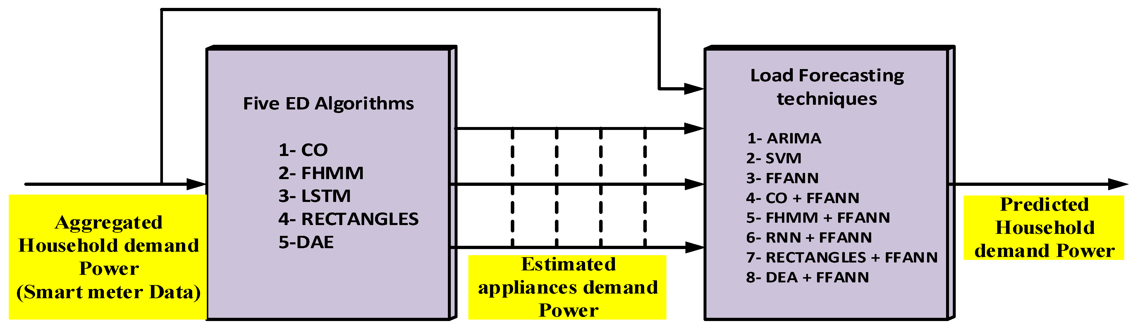
In this paper, an innovative methodology for STLF of household load demand is developed and employed. This approach is constructed from Feed-Forward Artificial Neural Network (FFANN), and a pre-processing Stage of Energy Disaggregation (SOED) based Data Mining Algorithms (DMA). This SOED extracts the individual appliances’ load demand profile from the aggregated household load demand to increase the training data window for the FFANN forecaster. These DMA include two bench-mark disaggregation algorithms (Factorial Hidden Markov Model (FHMM), Combinatorial Optimization) and three adopted Deep Neural Network (Long Short-Term Memory (LSTM), Denoising Autoencoder (DAE), and a network which regress start time, end time, and average power (RECTANGLES)). The proposed load forecasting approach outperforms the current state of the art techniques such as ARIMA, SVM, and FFANN regarding RMSE, NRMSE, and MAE. The main contributions of this paper are summarized in the following: (1) The improved forecasting architecture that combines the neural network and energy disaggregation to improve the forecasting for challenging load patterns such as household and small microgrid with high uncertainty and a small amount of historical data; (2) the second contribution of the paper is the detailed analysis and comparison of different disaggregation and forecasting algorithm; (3) the proposed algorithm target small microgrids and residential loads level. Improvement of the load forecasting for such loads is necessary for better energy management and demand-side management. The real-time pricing for such loads usually changes in hourly bases [
18,
19]. This paper is organized as follows:
Section 2 describes the energy disaggregation system and its implementation. In
Section 3, a description of the proposed Short-Term Load Forecasting approach is illustrated. In
Section 4, simulation results are presented and investigated to validate the proposed forecaster. Finally, in
Section 5, some conclusions are deduced from the developments in this paper.
2. Energy Disaggregation
Energy disaggregation (ED) is a computational approach for predicting the individual appliances power demand from a single meter which measures the aggregated power demand. George Hart starts this research in the mid-1980s [
20,
21]. His earliest research defined a signature taxonomy of feature. Nevertheless, his concentration was on extracting only transitions between steady-states. Consequent Hart’s clues, several ED procedures prepared for low-frequency data (1 Hz or slower) only to extract a minor number of features. There are numerous instances in the literature of manual feature extractors regarding the high-frequency sampling at kHz or even MHz. [
22,
23]. Hand-engineer feature extractors for instance Difference of Gaussians (DoG) and scale-invariant feature transform (SIFT) was the leading method to mine features for image classification before 2012 [
24]. However, in 2012, through the competition of ImageNet Large Scale Visual Recognition, several procedures achieved exceptional performance and did not use hand-engineered feature detectors. As an alternative, they used some disaggregation algorithms which automatically learned to extract a hierarchy of features from the raw image. In this paper, we will use five data mining algorithms for ED called CO, FHMM, DAE, LSTM, and RECTANGLES to extract the power demand profile for individual appliances from the main aggregated household power demand.
Figure 1 shows the block diagram of the whole proposed system. The full illustration of these algorithms presented later in this section. To use ED to enhance household forecasting performance, the energy consumption of each household must be available. Therefore, the dataset from the UK-DALE was used [
25]. Which is one of the first publicly available datasets collected essentially to support research on ED. It has a record of five houses. In our work, we will focus the study on only two houses. One of his recorded data was available during the training of the ED algorithm. However, the other was not seen during the training stage of the ED algorithm. Those five ED algorithms were implemented based on a toolkit called NILMTK [
26]. The code is written in Python which offers a massive set of libraries supporting both machine learning and ED algorithms.
2.1. Data Mining Disaggregation Algorithms
Five data mining disaggregation algorithms were used in this work. Two benchmark disaggregation algorithms; Factorial Hidden Markov Model (FHMM) and Combinatorial Optimization were utilized. Moreover, three adapted deep neural network architectures have been used for ED; (1) an exceptional form of a recurrent neural network (RNN) called long short-term memory (LSTM); (2) a network that produces rectangles for the estimated demand by regression of the start time, end time and average power demand (nicknamed by RECTANGLES); and (3) denoising autoencoder (DAE). The full illustration of these algorithms is presented later in this section.
2.1.1. Combinatorial Optimization
Optimization methods necessitate the presence of appliance signature libraries with all possible groupings of power demands of the appliances it desires to disaggregate. If we include the gatherings of all the connected appliances in a house, then this optimization approach is called brute-force. However, due to memory limitations as stated in [
27]. Brute-force methods are difficult to be applied to an embedded system. Therefore, the load identification requires the definition of an objective function and its minimization. Considering the aggregate data
and an appliance set
, the problem is formulated as [
27].
The Combinatorial Optimization is the most critical algorithm in this domain which minimizes the difference between the sum of the measure aggregate power and predicted appliance power [
28]. This technique was used by Hart in [
29]. The computational complexity is
, where
K is the number of appliance states,
N the number of appliances and
T the number of times slices used in the implementation. Consequently, the optimization approaches address mainly disaggregation for the most power-hungry devices. Reference [
30] discusses the two commonly cited disadvantages of this approach which are the decreasing of accuracy with the number of appliances and level of noise.
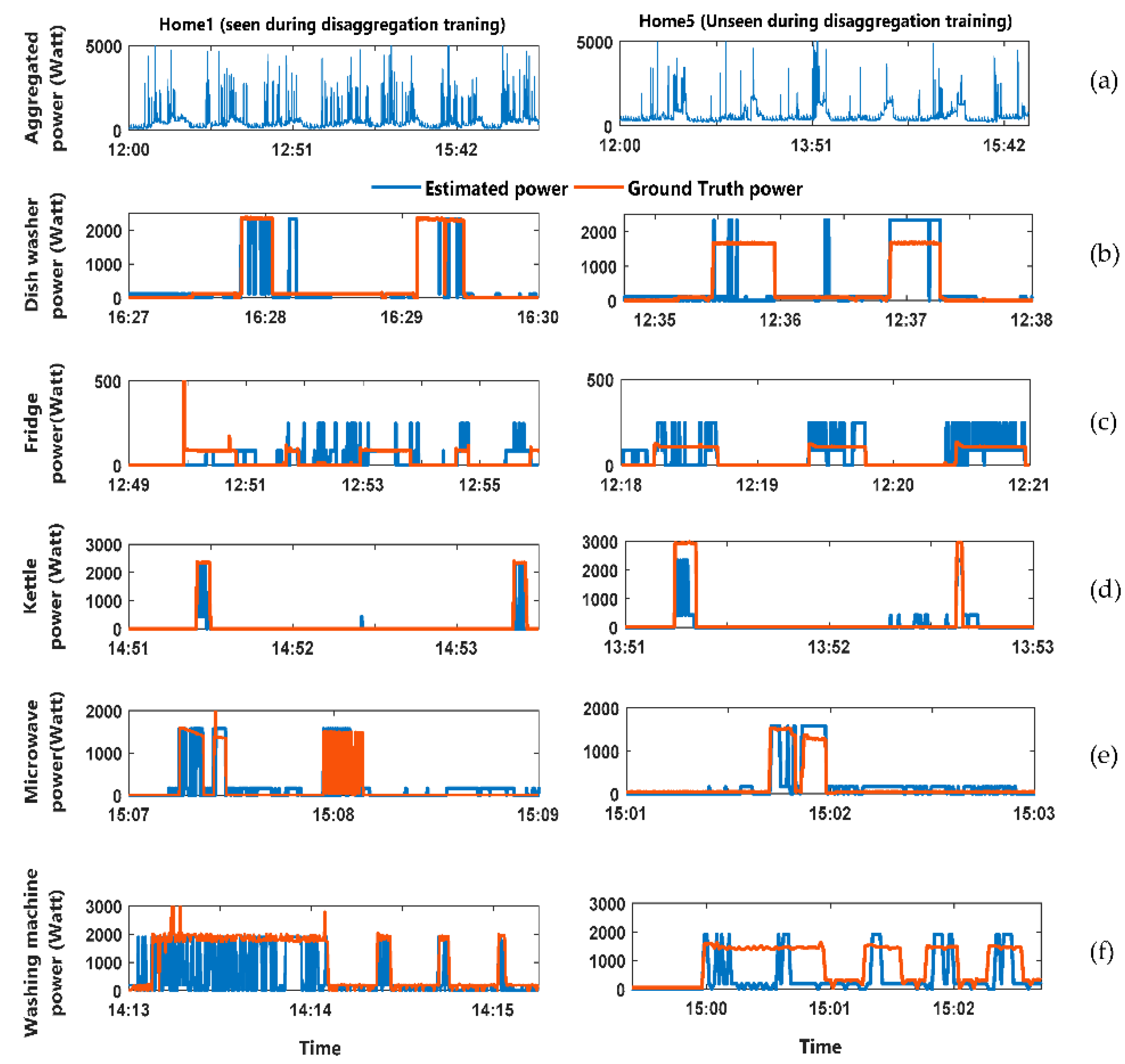
Figure 2 shows the output result of the CO energy disaggregation algorithm. The figure divided into two columns. The left hand side (LHS) column has the analysis for the home whose data was available during the training of the disaggregation algorithm. The right hand side (RHS) column has the analysis for the home whose data was not available during the training of the disaggregation algorithm. The figure have six rows described as follows: (a) Aggregated power consumption for the home; (b) comparison between the estimated and Ground truth power demand for the dishwasher; (c) comparison between the estimated and Ground truth power demand for the Fridge; (d) comparison between the estimated and Ground truth power demand for the Kettle; (e) comparison between the estimated and Ground truth power demand for the Microwave; (f) comparison between the estimated and ground truth power demand for the washing machine.
2.1.2. Factorial Hidden Markov Model
FHMM belong to the group of Temporal Graphical Models which is a class of probabilistic models. Such models have been applied previously to many real-world problems such as speech recognition. The most direct demonstration of sequence data is through the use of a Markov chain which is a sequence of discrete variables. The state transitions of devices are controlled by the hidden Markov model (HMMs) which is a statistical tool. Each variable is defined by its real power consumption in addition to other useful information such as duration of the on and off periods and time of use during the day/week. Thereby, at an instant of time t of a period
T,
t T, the aggregate consumption is
and needs to be broken down to the number of appliances
, where
t T and
n N with
N the number of appliances. The value of each device
at any time corresponds to one of the
K states of the trained model of the appliances [
27]. The mathematical representation of the a HMM represented by Equation (2) through Equation (6) [
27]. The behavior of a HMM can be completely defined and inferred by three parameters. First, the probability of each state of the hidden variable at the time
t can be represented by the vector
such that
Second, the transition probabilities from state
i at
t to state
j at
t + 1 can be represented by the matrix
A such that,
Third, the emission probabilities for
x are described by a statistical function with parameter
which is commonly assumed to be Gaussian distributed such that,
where
, and
are the mean and precision of a state’s Gaussian distribution. Finally, Equations (2)–(4) can be used to compute the joint likelihood of a HMM:
where the set of all model parameters which must be found for each appliance during the training phase is represented by
. Therefore, when applying an HMM for Energy Disaggregation, it is needed to tune the
parameters for each appliance during the training phase and afterwards, given a sequence of the power signal
to find the optimal sequence of discrete states
z. Their ability to handle daily operation consumption and the information about state transition of devices makes them a suitable solution for the problem. The complexity of the disaggregation using HMMs is
, where
K is the number of states of all the appliances and
T is the number of the time slices, i.e., how many times the algorithm is required to be applied [
27]. As it is shown the complexity is exponential with regard to the number of appliances while re-training is needed when a new group of appliances is added [
31].
The HMMs were used for appliance load recognition, and it was also shown that they are useful in the field of ED [
32]. Finally, HMMs is used to disaggregate an energy signal using generalized appliance model, and as a result, it was possible to extract consumption of individual devices without any manual labeling [
25]. Nevertheless, the author uses low-frequency smart meter data because of lack of high-frequency data and smart metering infrastructure supporting such high rates. Although the HMM is a powerful technique, the method for the inference of hidden states is often affected by local minima [
33]. To overcome this limitation, variants of HMMs are used such as the Factorial HMM (FHMM). The concept is that the output is an additive function of all the hidden states. In the model, each observation is dependent upon multiple unknown variables [
34]. Likewise, the joint likelihood of an FHMM as stated in [
35] is computed by,
where 1:
N symbolizes a sequence of appliances 1, …,
N. However, the computational complexity of both learning and disaggregating is greater for FHMMs compared to HMMs. This is due to the conditional dependence of the Markov chains.
Figure 3 shows the output result of the FHMM energy disaggregation algorithm. The figure divided into two columns. The LHS column has the analysis for the home whose data was available during the training of the disaggregation algorithm. The right-hand side (RHS column have the analysis for the home whose data was not available during the training of the disaggregation algorithm. The figure has six rows described as follows: (a) Aggregated power consumption for the home; (b) comparison between the estimated and Ground truth power demand for the dishwasher; (c) comparison between the estimated and ground truth power demand for the fridge; (d) comparison between the estimated and ground truth power demand for the kettle; (e) comparison between the estimated and Ground truth power demand for the microwave; (f) comparison between the estimated and Ground truth power demand for the washing machine.
2.1.3. Denoising Autoencoder
It is an autoencoder which attempts to reconstruct a clean target from a noisy input. DAEs are typically trained by an artificially corrupting signal before it goes into the net’s input, where the net’s target is the clean signal. In ED, we consider the corruption as being the power demand from the other appliances. So we do not add noise artificially. Instead, we use the aggregate power demand as the (noisy) input to the net and ask the net to reconstruct the clean power demand of the target appliance.
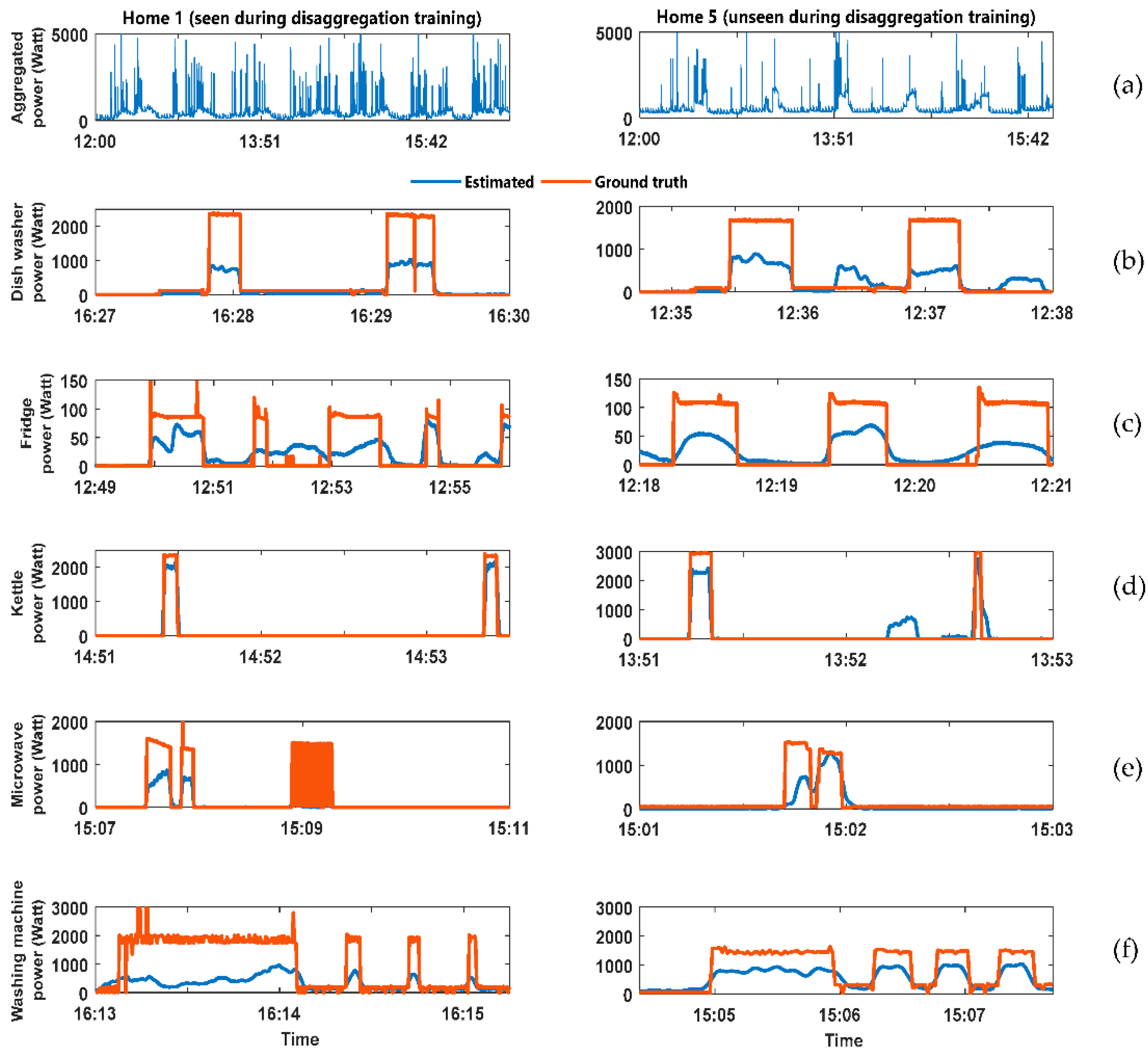
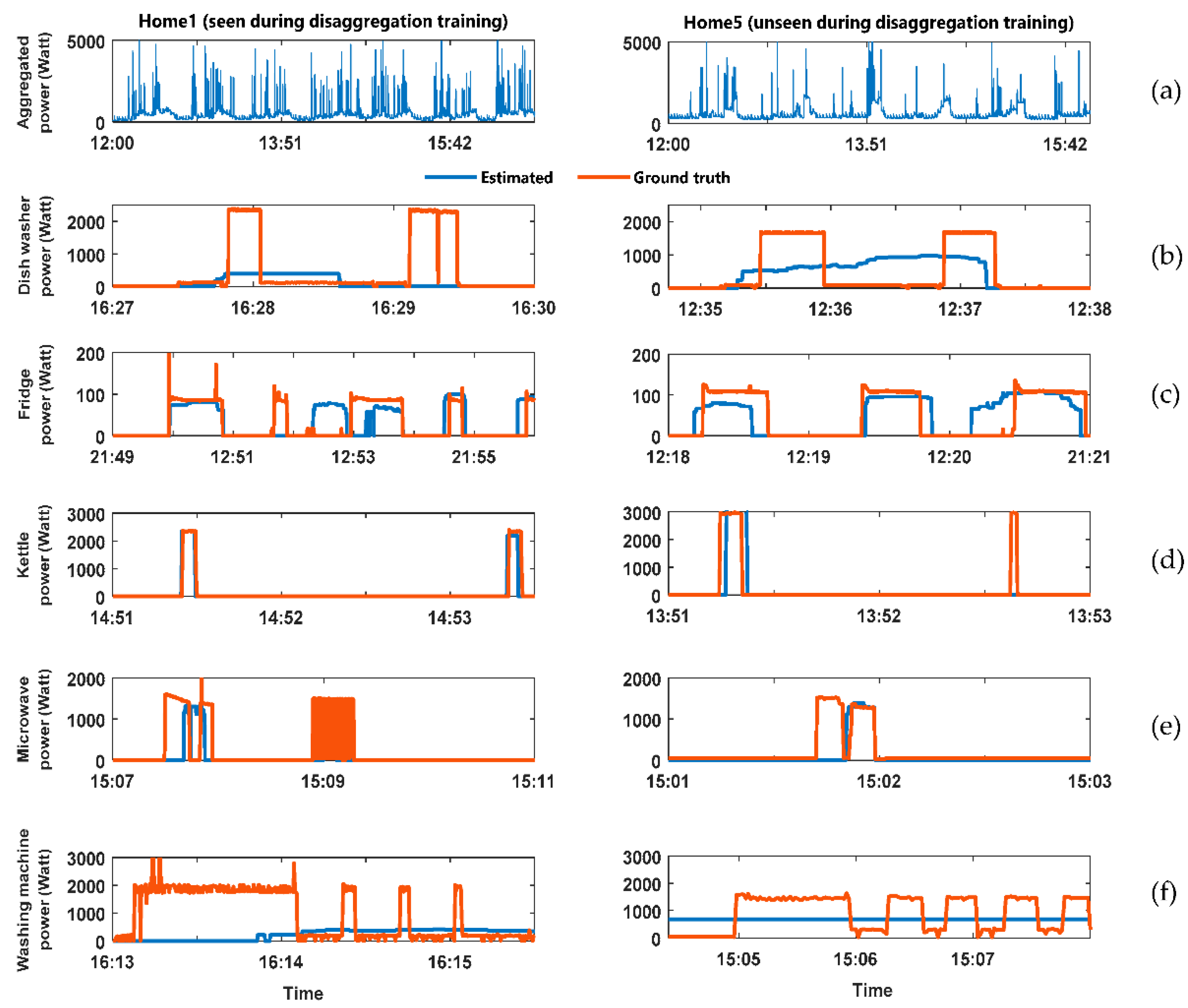
Figure 4 shows the output result of the DAE energy disaggregation algorithm. The figure divided into two columns. The LHS column has the analysis for the home whose data was available during the training of the disaggregation algorithm. The right-hand side (RHS column have the analysis for the home whose data was not available during the training of the disaggregation algorithm. The figure has six rows described as follows: (a) Aggregated power consumption for the home; (b) comparison between the estimated and ground truth power demand for the dishwasher; (c) comparison between the estimated and ground truth power demand for the fridge; (d) comparison between the estimated and ground truth power demand for the kettle; (e) comparison between the estimated and ground truth power demand for the microwave; (f) comparison between the estimated and ground truth power demand for the washing machine.
2.1.4. Regress Start Time, End Time, and Average Power (RECTANGLES)
This algorithm draws a rectangle around each appliance activation in the aggregate data where the left side of the rectangle is the start time, the right side is the end time, and the height is the average power demand of the appliance between the start and end times.
Figure 5 shows the output result of the DAE energy disaggregation algorithm. The figure divided into two columns. The LHS column has the analysis for the home that its data was available during the training of the disaggregation algorithm. The right-hand side (RHS column have the analysis for the home whose data was not available during the training of the disaggregation algorithm. The figure has six rows described as follows: (a) Aggregated power consumption for the home; (b) comparison between the estimated and ground truth power demand for the dishwasher; (c) comparison between the estimated and ground truth power demand for the fridge; (d) comparison between the estimated and ground truth power demand for the kettle; (e) comparison between the estimated and ground truth power demand for the microwave; (f) comparison between the estimated and ground truth power demand for the washing machine.
2.1.5. Recurrent Neural Network (RNN or LSTM)
A recurrent neural network (RNN) is a type of artificial neural network where relations between units form a directed graph along a sequence. This allows it to exhibit dynamic temporal behavior in a time sequence. Different from feedforward neural networks, RNNs can use their internal memory to process sequences of inputs.
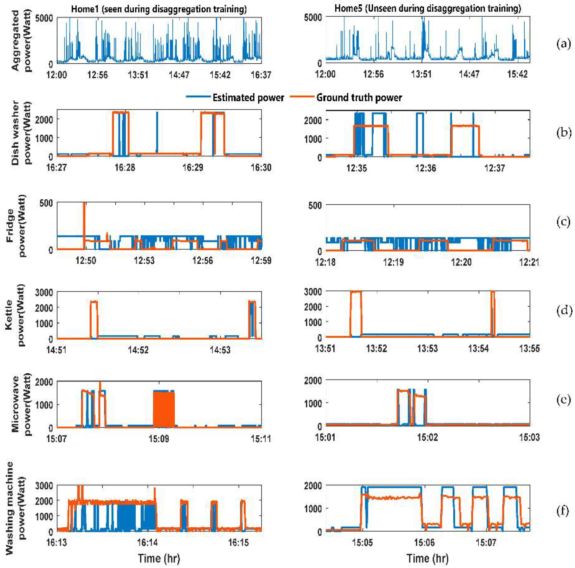
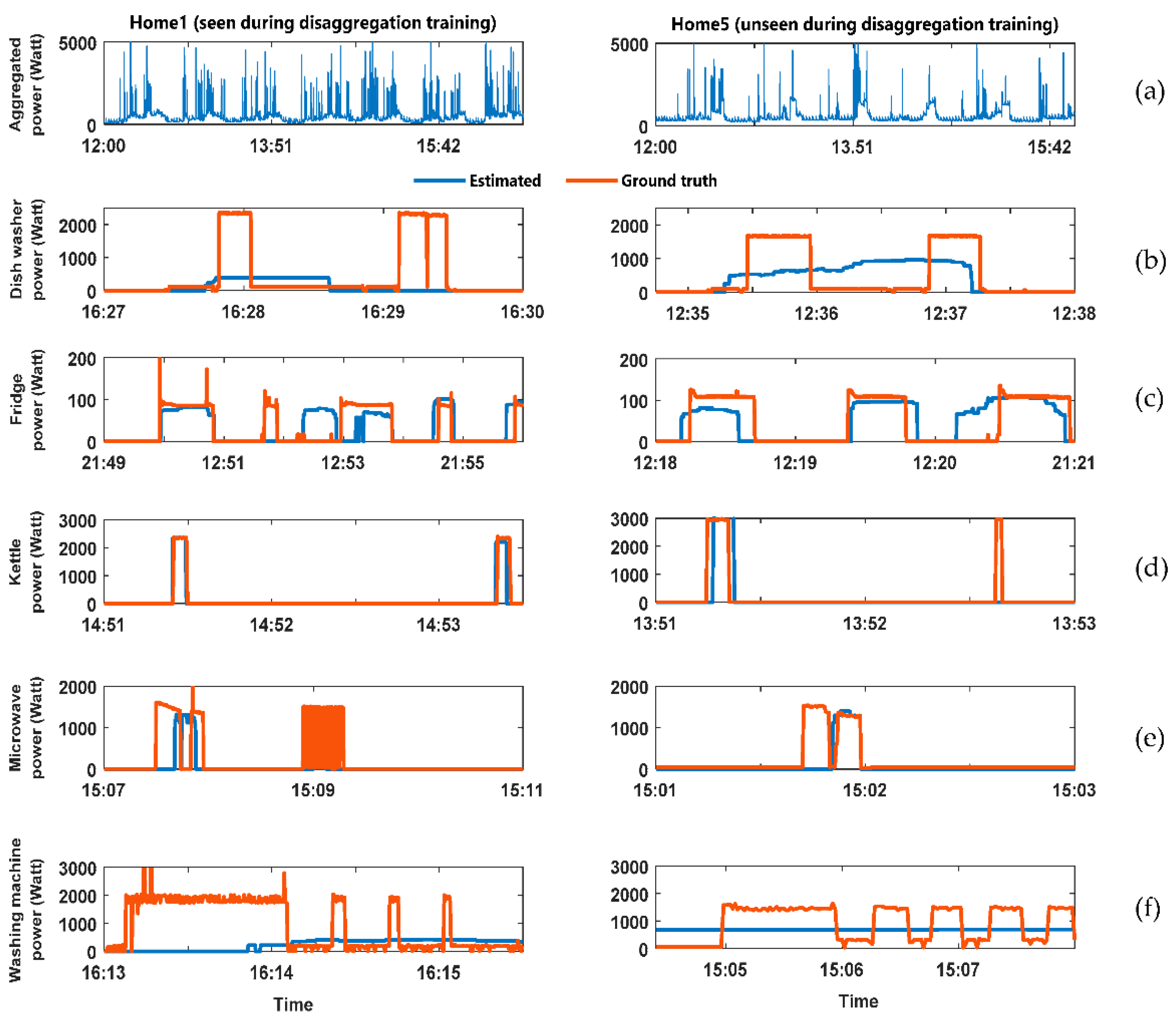
Figure 6 shows the output result of the LSTM energy disaggregation algorithm. The figure is divided into two columns. The LHS column has the analysis for the home whose data was available during the training of the disaggregation algorithm. The right-hand side (RHS column have the analysis for the home whose data was not available during the training of the disaggregation algorithm. The figure has six rows described as follows: (a) Aggregated power consumption for the home; (b) comparison between the estimated and ground truth power demand for the dishwasher; (c) comparison between the estimated and ground truth power demand for the fridge; (d) comparison between the estimated and ground truth power demand for the kettle; (e) comparison between the estimated and ground truth power demand for the microwave; (f) comparison between the estimated and ground truth power demand for the washing machine.
Table 1, summarize the compression for the disaggregating algorithms and its performance to for the seen and unseen data provided in
Figure 2,
Figure 3,
Figure 4,
Figure 5 and
Figure 6.
2.2. Disaggregation Stage Analysis
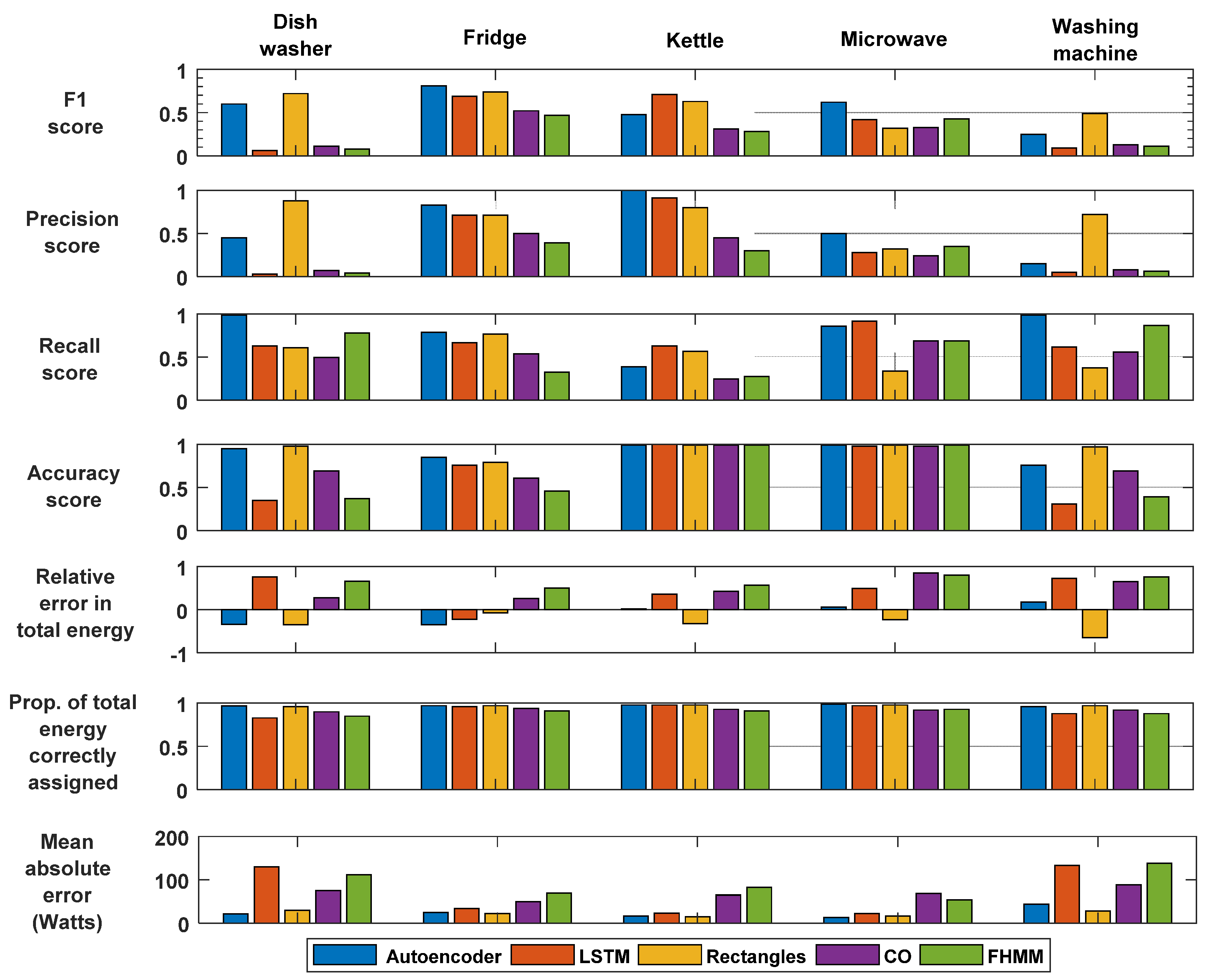
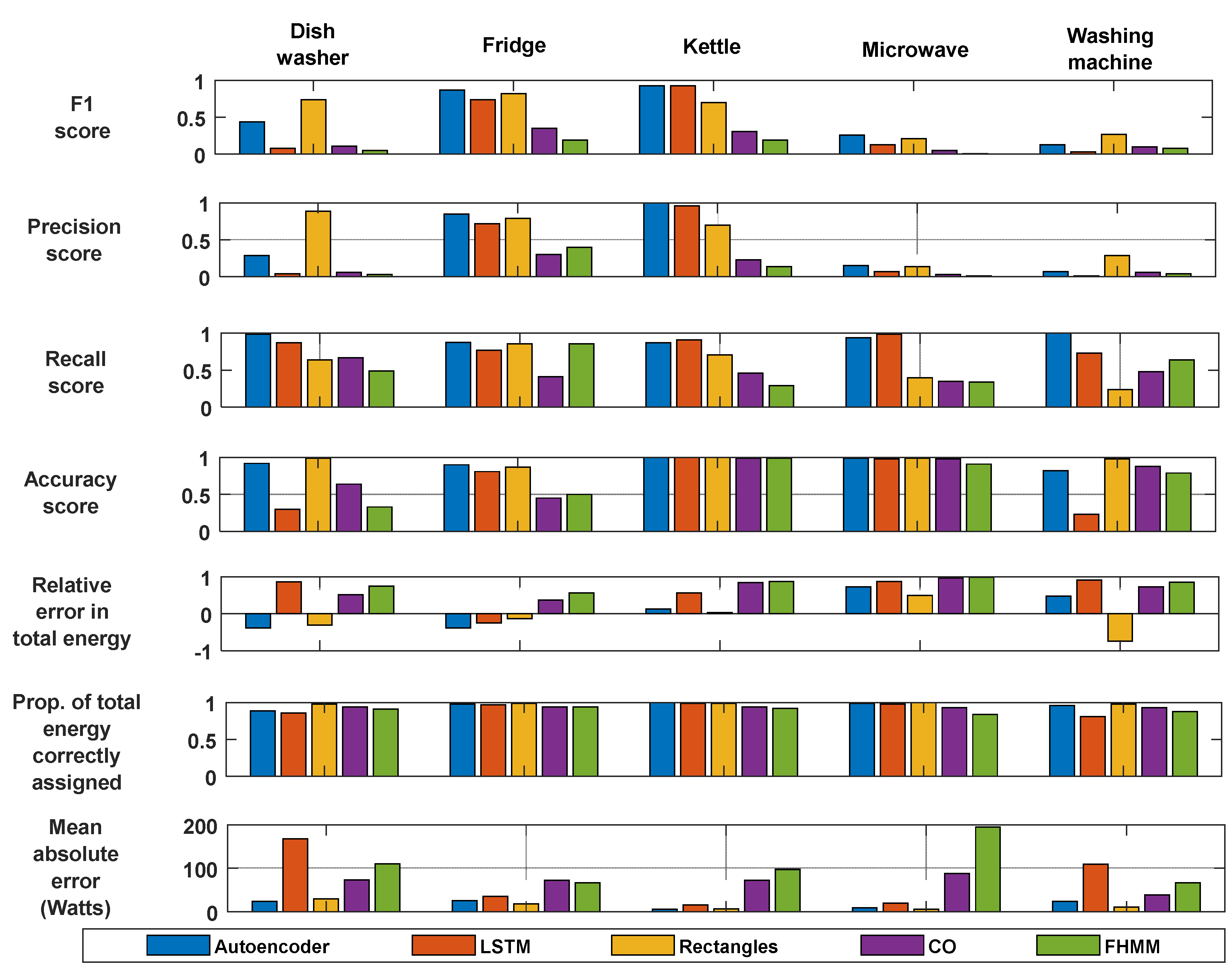
To identify the best disaggregation algorithm was used in the ED stage. Seven common classification metrics represented through Equations (7)–(23). These seven different accuracy measures are the well-known metrics for evaluating the energy disaggregation techniques [
36,
37].
Figure 7 shows the comparison between the disaggregation analyses for the home which was seen during training.
Figure 8 shows the comparison between the disaggregation analyses for the home which was unseen during training. The denoising autoencoder and RECTANGLES outperform LSTM, FHMM, and CO in most of the metrics throughout the five appliances.
Figure 7 and
Figure 8 are divided into five columns and seven rows. The five columns represent five appliances labeled from the left as follows: Dishwasher; fridge; kettle; microwave; washing machine. The seven rows labeled from upper to lower as follows: F1 score Equation (14); precision score Equation (13); recall score Equation (12); accuracy score Equation (15); relative error in total energy Equation (21); proportion of total energy correctly assigned Equation (23); mean absolute error Equation (22). Therefore, the result at position (1, 1) represents the F1 score for the dishwasher with five different data mining energy disaggregation algorithms. These five algorithms were the legend at the footer of the figures.
3. The Implemented Short-Term Load Forecasting
A feed-forward Neural Network using the Levenberg-Marquardt backpropagation algorithm was employed. The Neural network consists of one input layer, three hidden layers, and one node at the output layer to predicted the aggregated power demand for an hour ahead. The input layer has eleven inputs which match the data utilized for load prediction. These input data consists of (five inputs from the disaggregation stage and six inputs from the aggregated demand of the home for the current and previous hours of historical data. The five inputs represent the load demand of the five major appliances in the home at the present hour which extracted from the energy disaggregation stage (dishwasher, fridge, kettle, microwave, and washing machine). The six inputs represent the current and historical consumption hours. Three inputs include the current hour power demand, one for an hour before, one for two hours earlier, and another three inputs include one for a day earlier, one for the 23 h earlier, and one for 22 h earlier. The reason for selecting six inputs from the aggregated data is that we picked two groups of three inputs. One group will cover the most recent three hours, and the other group covers the early three hours in the last 24 h. Each three inputs will cover three hours to cover double of the maximum interval of the time cycle of the washing machine which has the tallest time interval reach to 90 min [
25]. Regarding the data structure, there are significant changes in the inputs and output ranges. Thus, all the input and output data have been normalized to avoid saturation of the FFANN. Normalization is done using Equation (24).
where
is the normalized power value,
is the actual power value,
is the peak power. For training, validation, and testing of the neural network, the data divided to 70% for training, 15% for validating, and 15% for testing.
In many ways, this test network presents a challenging forecasting case, and these are all drawn from the real UK dataset.
4. Simulation Results
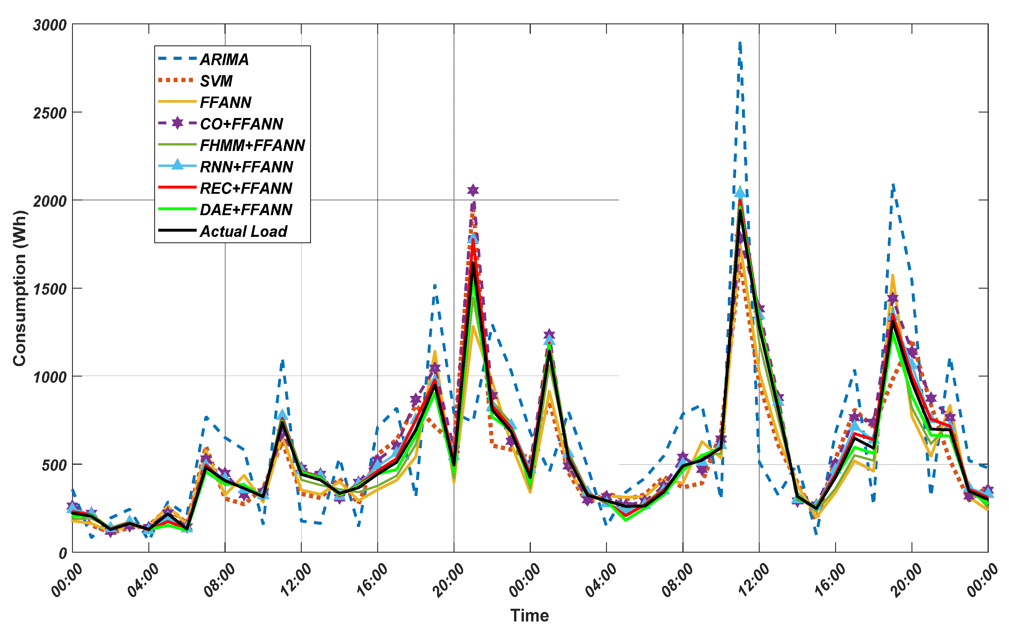
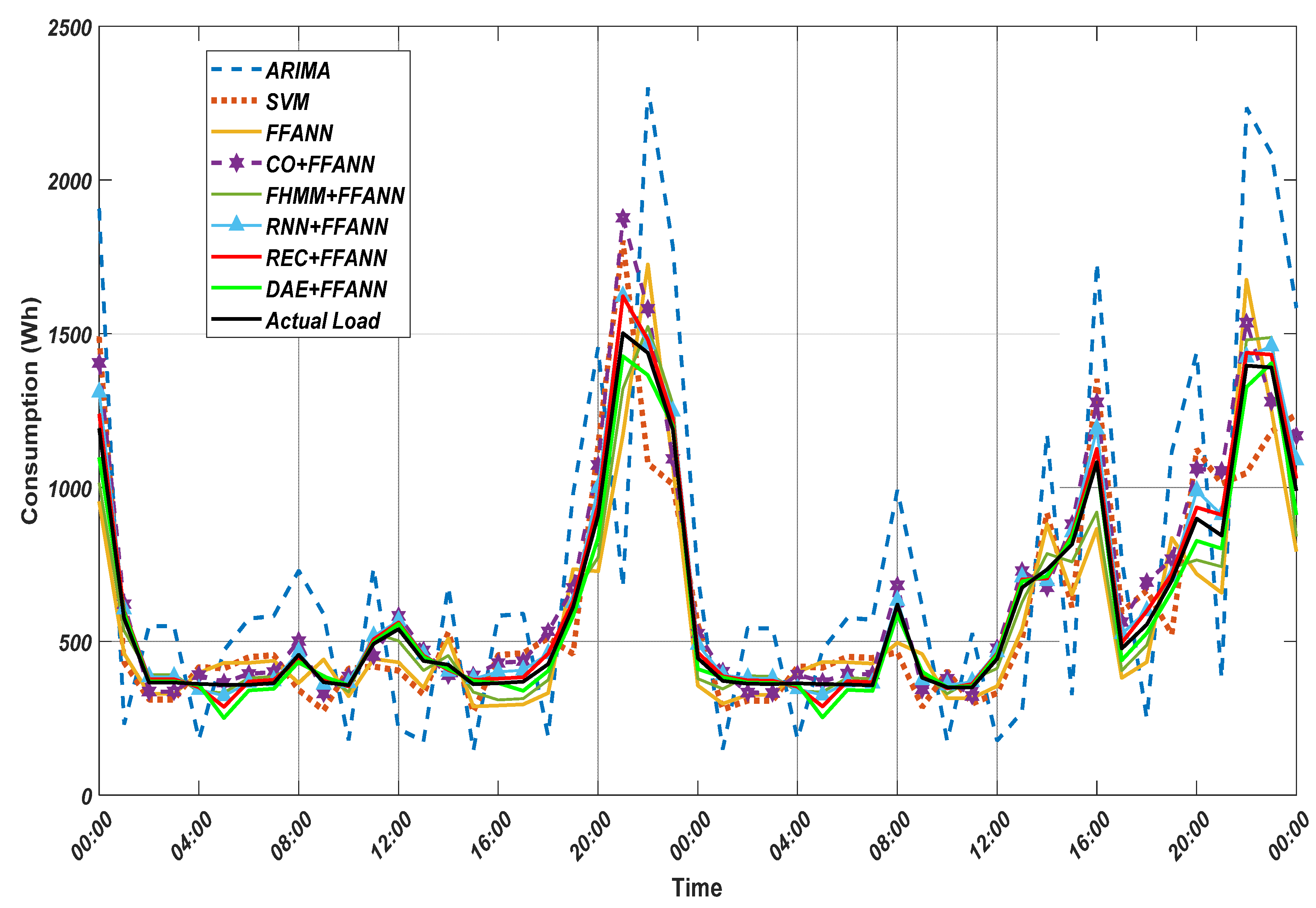
Figure 9 and
Figure 10 demonstrate the actual load and the forecasted load by different methods for the home seen during the ED training and unseen during ED training, respectively. In order to assess the performance of the proposed method in conducting STLF for residential households, three widely used metrics were employed, including root mean squared error (RMSE), normalized root mean squared error, and mean absolute error. The three performance metrics are introduced in Equations (25)–(27). These three metrics describe the performance of the forecaster from different view [
38,
39]. The RMES is good for getting average error considering the error direction. In another word, the RMSE can give the idea about the average error between the predicted and actual signal regardless of the direction of the error. Additionally, the NRMSE gives the same description, but by normalized values which allows the comparison between different systems (two home with two different power rating). However, the MAE gives the average error over a period concerning the direction which could give a good idea of the accumulated error in the forecasted energy.
Table 2 and
Table 3 compare the performance of the proposed approach regarding RMSE, NRMSE, and MAE with the current state of the art techniques, i.e., AIRMA, SVM, and FFANN. As illustrated, the five proposed approaches; DAE + FFANN, REC + FFANN, RNN + FFANN, FHMM + FFANN, and CO + FFANN outperform FFANN, SVM, and ARIMA in all metrics used. In case of
Table 2 which should be the worst because the data was unseen during the energy disaggregation stage. The proposed (REC + FFANN) brings 91.13% reduction in RMSE and NRMSE, 92.36% reduction of MAE as compared with ARIMA.
5. Conclusions
In this paper, an improved load demand forecasting technique utilizing a preprocessing stage of energy disaggregation techniques combined with FFANN are proposed. This proposed approach implemented for household’s STLF under high uncertainty and volatility associated with customer behavior which is difficult to predict. Five different energy disaggregation techniques; DAE, RECTANGLES, RNN, FHMM, and CO were implemented and evaluated for a data of two different homes. Seven performance metrics were utilized to benchmark the implemented energy disaggregation techniques to give a comprehensive comparison of the performance of the techniques being assessed. The proposed STLF approaches; RECTANGLES + FFANN, DAE + FFANN, RNN + FFANN, FHMM + FFANN, and CO + FFANN outperform FFANN, SVM, and ARIMA in all three benchmark metrics have usually been used in literature to evaluate the performance of STLF. The best approach used for energy disaggregation is denoising autoencoder which directly affected the performance of the STLF at residential household level. A great comparison and performance analysis show that the proposed technique (DEA + FFANN) brings 91.13% reduction in RMSE and NRMSE, 92.36% reduction of MAE as compared to ARIMA.


